A Graphical Representation of Equivalence Classes of AMP Chain Graphs

A Graphical Representation of Equivalence Classes

of AMP Chain Graphs

Alberto Roverato [email protected]

Department of Social, Cognitive and Quantitative Sciences University of Modena and Reggio Emilia

Viale Allegri 9

I-42100 Reggio Emilia, Italy

Milan Studen´y [email protected]

Institute of Information Theory and Automation Academy of Sciences of the Czech Republic Pod vod´arenskou vˇeˇz´ı 4

18208 Prague 8 Libeˇn, Czech Republic

Editor: David Madigan

Abstract

This paper deals with chain graph models under alternative AMP interpretation. A new represen-tative of an AMP Markov equivalence class, called the largest deflagged graph, is proposed. The representative is based on revealed internal structure of the AMP Markov equivalence class. More specifically, the AMP Markov equivalence class decomposes into finer strong equivalence classes and there exists a distinguished strong equivalence class among those forming the AMP Markov equivalence class. The largest deflagged graph is the largest chain graph in that distinguished strong equivalence class. A composed graphical procedure to get the largest deflagged graph on the basis of any AMP Markov equivalent chain graph is presented. In general, the largest deflagged graph differs from the AMP essential graph, which is another representative of the AMP Markov equiva-lence class.

Keywords: chain graph, AMP Markov equivalence, strong equivalence, largest deflagged graph,

component merging procedure, deflagging procedure, essential graph

1. Introduction

More recently, another interpretation of chain graphs was introduced by Andersson, Madigan and Perlman (1996); see also Andersson et al. (2001). This interpretation leads to an alternative Markov property and we will refer to it as the AMP Markov property.

Two different chain graphs may be equivalent with respect to a considered Markov property, by which is meant that they define the same statistical model. The distinction between different interpretations of chain graphs is reflected by the different concepts of equivalence, namely the LWF Markov equivalence and the AMP Markov equivalence.

From a statistical perspective, the point of interest is a statistical model. However, if we repre-sent a statistical model using an arbitrary graph in the respective Markov equivalence class, then the non-unique nature of graphical description may result in difficulties. One type of difficulty concerns problems one can meet in structural learning of graphical models; see Section 2.3 of Chickering (2002) for a review in the case of acyclic directed graphs. A solution to these problems may be provided by a suitable choice of a unique representative of each Markov equivalence class, that is, of a particular element in that equivalence class. The choice of a suitable representative is also important from the perspective of causal inference in chain graphs (Lauritzen, 2001, Section 11.2). The problem of the representative choice has a natural solution in the LWF case. Frydenberg (1990) showed that every LWF equivalence class contains the largest chain graph, which is the graph with the largest amount of undirected edges within the LWF equivalence class. Furthermore, every arrow in the largest chain graph is an arrow with the same direction in every chain graph from the class. The largest chain graph is uniquely determined and can serve as a natural representative of the LWF equivalence class. Moreover, there exist at least two procedures that transform every chain graph into the largest chain graph of the respective LWF equivalence class Roverato (2005); Volf and Studen´y (1999).

However, the situation is different in the AMP case. It is not clear what is a natural representative of an AMP equivalence class and, in particular, the notion of the “largest AMP chain graph” makes no sense. Andersson et al. (2001) proposed to represent an AMP equivalence class by a so-called AMP essential graph. Every arrow in the AMP essential graph is either an arrow with the same direction or an undirected edge in every chain graph from the equivalence class. Their terminology was inspired by the case of acyclic directed graph models, in which case the corresponding equiva-lence class has a suitable representative called the essential graph (Andersson et al., 1997). Indeed, if an AMP equivalence class contains an equivalence class of acyclic directed graphs, then the AMP essential graph coincides with the respective essential graph; see Proposition 4.2 in Andersson and Perlman (2006). However, as of now, there is no algorithm to construct the AMP essential graph, as in the LWF case. Furthermore, in the case that the AMP equivalence class contains a completely undirected graph, it may happen that the AMP essential graph has some arrows, and this unpleasant phenomenon was already reported in Section 7 of Andersson et al. (2001).

graph because then, as one would expect, that undirected graph coincides with our largest deflagged graph.

These are the main contributions of the paper:

1. We introduce a new concept, namely, the concept of strong equivalence of chain graphs. An important observation is that every AMP equivalence class of chain graphs decomposes into strong equivalence classes.

2. Every strong equivalence class has a unique representative given by the largest chain graph of the class. We introduce a procedure, called the component merging procedure, which starts from any chain graph G and, by replacing arrows with undirected edges, finds the largest graph in the class of chain graphs strongly equivalent to G.

3. There exists a unique distinguished strong equivalence class among those forming an AMP equivalence class. Its elements have the largest amount of immoralities and the least possible amount of flags. We call the graphs in this class the maximally deflagged graphs, briefly the deflagged graphs. We introduce a procedure, called the deflagging procedure, which starts from any chain graph G and, by replacing undirected edges with arrows, produces a deflagged graphG AMP equivalent to G.b

4. We propose to characterize every AMP equivalence class by means of the respective largest deflagged graph. This representative can be constructed by applying the component merging procedure to the chain graphG obtained by the deflagging procedure.b

The next section recalls basic graphical concepts. Then, in Section 3, the main results in the LWF case are recalled in order to let the reader see some analogy. In Section 4, we give an overview of our new results and illustrate them by an example. The results on strong equivalence of chain graphs are formulated in Section 5. They appear to be analogous to the results valid in the LWF case. In Section 6, we present a deflagging procedure to get a deflagged graph in a given AMP equivalence class. Section 7 contains some concluding remarks. Proofs of the main results are moved to the Appendix.

2. Basic Concepts

In this paper we consider graphs that admit both directed edges, called arrows, and undirected edges, called lines. Formally, given a non-empty finite set N, an arrow over N is an ordered pair (a,b)of distinct elements of N and a line over N is a subset{a,b}of N of cardinality two, that is, an unordered pair of distinct elements of N. A hybrid graph is a triplet H ≡(N,

A

,

L

) where N is a finite non-empty set of nodes,

A

a set of arrows over N and

L

a set of lines over N such that no multiple edges are allowed, which means that if(a,b)∈

A

then(b,a)6∈

A

and{a,b} 6∈

L

. To express that N is the set of nodes of H we also say that H is a hybrid graph over N.

A set of nodes C⊆N is connected in H if, for every a,b∈C, there exists an undirected path connecting them, that is, a sequence of distinct nodes a=c1, . . . ,cn=b, n≥1 such that ci−−−ci+1 in H for i=1, . . . ,n−1. A (connectivity) component in H is a maximal connected set in H with respect to set inclusion. Evidently, components in a hybrid graph are pairwise disjoint.

Given a set of nodes A⊆N in a hybrid graph H, the set of parents of nodes in A, denoted by pa_H(A), is the set

pa_H(A)≡ {b∈N ; b−→a in H for some a∈A}.

A descending path in H from a node a to a node b is a sequence of distinct nodes a=c1, . . . ,cn=b, n≥1 such that either ci−→ci+1in H or ci−−−ci+1in H for i=1, . . . ,n−1. If there exists a path of this kind in H then we say that a is an ancestor of b in H. The set of ancestors in H of nodes in a set A⊆N will be denoted by anH(A); observe that one has A⊆anH(A).

An undirected graph is a hybrid graph without arrows, that is,

A

=/0. A set K⊆N is complete in an undirected graph H if,∀a,b∈K, a6=b, one has a−−−b in H. Given a hybrid graph H over N, the respective underlying graph is an undirected graph Huover N such that a−−−b in Hu iff[a,b] is an edge in H.

A directed graph is a hybrid graph without lines, that is,

L

=/0. A directed graph H is acyclic if there is no directed cycle in H, that is, there is no sequence of nodes d0, . . . ,dn−1,dn=d0, n≥3 such that d0, . . . ,dn−1are distinct and,∀i=0, . . . ,n−1, di−→di+1in H.

The concept of a chain graph (CG) can be introduced in two equivalent ways. Note that we are going to use the abbreviation CG in the rest of the paper. The first definition is that a CG is a hybrid graph H whose components can be ordered to form a chain, that is, a sequence C1, . . . ,Cm, m≥1 such that

• if a−−−b in H then a,b∈Cifor some i,

• if a−→b in H then a∈Ci,b∈Cjwith i< j.

Note that this is the reason for which some authors call the components in a CG chain components. A consequence of this definition is that every CG has a terminal component, that is, a component T such that there is no arrow a−→ b in H with a∈T . The other definition is that a CG is a hybrid graph H without semi-directed cycles. A semi-directed cycle of the length n is a sequence of nodes d0, . . . ,dn−1,dn=d0 with n≥3 such that d0, . . . ,dn−1 are distinct, d0−→d1 in H and, ∀i=1, . . . ,n−1, either di−→di+1in H or di−−−di+1in H. See Lemma 2.1 in Studen´y (1997) for the proof of equivalence of both definitions of a CG. It is easy to see that every undirected graph and every acyclic directed graph is a CG.

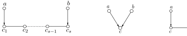
a b

c₁ c₂ cs₋₁ cs

a b

c

a

b c

Figure 1: A complex, an immorality and a flag.

A flag in a hybrid graph H is another induced subgraph of H for three nodes, namely a−→ c−−−b where a,b,c are distinct nodes and[a,b]is not an edge in H. An example of a flag is shown in the right-hand picture of Figure 1. A triplex in a hybrid graph H is a pair h{a,b},cisuch that either a−→c←−b is an immorality in H, a−→c−−−b is a flag in H or a−−−c←−b is a flag in H. All three different versions of a triplex are shown in Figure 2. Two CGs G and H over N will be called triplex equivalent iff they have the same underlying graph and triplexes. Note that coincidence of triplexes is understood as follows. If, for instance, a−→c←−b is an immorality in G then it need not be an immorality in H but it has to be one of three versions of the triplex

h{a,b},ci. Given a CG H, the class of CGs that are triplex equivalent to H will be denoted byH.

3. Representation of LWF Equivalence Classes

In this section we recall known results concerning the LWF case. The aim is to help the reader to realize the analogy between these former results and our new results on strong equivalence of CGs presented in Section 5. Moreover, an overview of the results in the LWF case will indicate what is the main difference from the AMP case, which is reported in Section 4.

3.1 Largest Chain Graph in a LWF Equivalence Class

In this paper, we omit the formal definition of LWF Markov property and LWF Markov equivalence; this can be found in Frydenberg (1990). Instead, we recall Frydenberg’s graphical characterization of LWF equivalence of CGs (see Proposition 5.6 in Frydenberg, 1990). He showed that two CGs over the same set of nodes are LWF Markov equivalent iff they are complex equivalent.

The second crucial point is that every LWF equivalence class is endowed with a natural partial ordering. Supposing that H= (N,AH,LH)and G= (N,

A

G,

L

G)are two LWF equivalent CGs, we say that H is larger than G if

A

H⊆

A

G, that is

a−→b in H implies a−→b in G, (1)

a c b a c b a c b

(i) (ii) (iii)

for every pair a and b of distinct nodes in H. Observe that the fact that G and H have the same underlying graph necessitates that

L

G⊆

L

H, that is

a−−−b in G implies a−−−b in H, (2)

which means H has ‘more’ lines than G. One can easily show that the relation defined by (1) is a partial ordering on every LWF equivalence class; we will write H≥G if (1) is fulfilled.

Third, Frydenberg also showed (Proposition 5.7 of Frydenberg, 1990) that every LWF equiv-alence class

G

has the largest element with respect to this ordering, that is, G_∞∈

G

such that for every G in

G

one has G∞≥G. Thus, this graph G∞, named the largest chain graph of

G

, can serve as a natural representative of

G

.

3.2 Feasible Merging of Components

The last important point is that there are procedures which allow one to get the largest CG G∞∈

G

on the basis of any CG G∈

G

from the LWF equivalence class. At least three procedures of this kind have been presented in the literature; however, two of them are methodologically equivalent.

One of them could be a procedure based on Theorem 3.9 of Volf and Studen´y (1999). The basic idea is that some arrows in a CG G∈

G

are indicated as ‘protected’ arrows. Then all arrows in G which are not ‘protected’ are replaced with lines and the largest chain graph G∞of

G

is obtained.

Another procedure, called the pool-component rule, was presented in Section 5 of Studen´y (1997). The basic idea is that there is an elementary operation of merging components in a CG whose result is an LWF equivalent CG. By consecutive application of this operation, the respective largest chain graph can be obtained. However, the formal description of that elementary operation given in Studen´y (1997) is still awkward.

The third procedure is described in Roverato (2005). Its basic idea is essentially the same; an elementary step of that procedure consists of merging components of an ‘insubstantial’ meta-arrow, that is, of the bunch of arrows between two certain components. It is shown in Section 4 of Roverato (2005) that, by consecutive application of that elementary step, the respective largest CG is obtained. One can show that the elementary operations presented in Studen´y (1997) and Roverato (2005) are equivalent (see Studen´y et al., 2006), but the formal description of the operation presented in Roverato (2005) is much more elegant from the mathematical point of view. We decided to take it as the basis of the following definitions.

Definition 1 (meta-arrow)

Let G be a CG. A pair of components(U,L)in G such that there exists an arrow a−→b in G with a∈U and b∈L determines a meta-arrow in G. More specifically, the meta-arrow is the collection of all arrows a−→b with a∈U and b∈L. The component U will be called the upper component and the component L the lower component (of the meta-arrow). We will occasionally use the notation U⇉L.

(M1)

L

U =⇒ _U

L

(M2)

U

L

=⇒

U

L

Figure 3: Two examples of feasible merging. The vertices belonging to the set K from (i) are filled in and arrows of the meta-arrow U⇉_{L are bold.}

in a CG, we have decided to simplify our terminology. Our additional assumption also implies that the considered components U and L are different.

Definition 2 (merging of components)

By merging of components in a CG G we understand the following operation applicable to G. Given a pair of components(U,L)which defines a meta-arrow, we replace all arrows of the meta-arrow U⇉_{L with lines and say that the resulting hybrid graph G}′_{is obtained by merging of components} U and L; more specifically, by merging of the upper component U and the lower component L.

Note that the above terminology was inspired by terminology from Studen´y (2004). In general, the result of the operation of merging components in a CG need not be a CG. However, there are sufficient conditions for this; one of them is as follows.

Definition 3 (feasible merging)

Let(U,L)be a pair of components in a CG G that defines a meta-arrow in G. We say that merging of components U and L is feasible (in G) if the following two conditions hold:

(i) K≡ pa_G(L)∩U is a complete set in G,

(ii) ∀b∈K pa_G(L)\U⊆pa_G(b).

It is shown in Section 4 of Roverato (2005) that a hybrid graph G′ obtained from a CG G by feasible merging of its components is a CG complex equivalent to G; actually, it is shown there that the requirements (i) and (ii) together establish a necessary and sufficient condition for this. In fact, that is the reason we decided to name this operation with CGs “feasible merging of components’’ because the condition ensures that one remains in the same LWF equivalence class of CG after the merging operation. Moreover, it is also proven in Roverato (2005) that, by repeated application of this operation to a CG G∈

G

, the respective largest CG G_∞∈

G

is obtained.

4. Representation of AMP Equivalence Classes

In this section we reveal the internal structure of AMP Markov equivalence classes. First, we recall the graphical characterization of AMP equivalence. Then we introduce a special kind of equivalence of CGs, called strong equivalence, such that every AMP equivalence class decomposes into strong equivalence classes. Basic results on strong equivalence are postponed to Section 5. The next step is to introduce a special flag ordering between strong equivalence classes within a fixed AMP equivalence class. We show that the smallest element with respect to that ordering exists and, finally, we propose to represent the whole AMP equivalence class by a natural representative of that distinguished strong equivalence class, called largest deflagged graph.

4.1 Graphical Characterization of AMP Equivalence

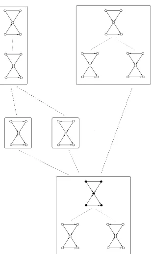
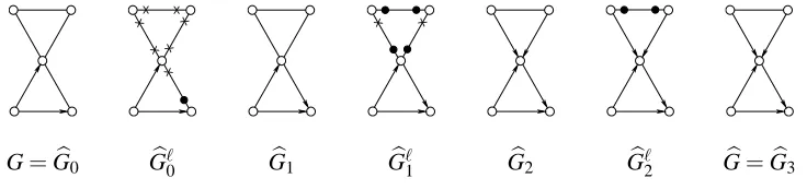
The formal definitions of AMP Markov property and AMP Markov equivalence are omitted; they can be found in Andersson et al. (2001). Here we recall graphical characterization of AMP equiv-alence given by Andersson et al. (2001, Theorem 5). They showed that two CGs over the same set of nodes are AMP Markov equivalent iff they are triplex equivalent. An example of an AMP equivalence class is given in Figure 2. A further, less trivial, example containing ten CGs is given in Figure 4.

Given a CG H, let us consider the setHof all CGs triplex equivalent to H. If we consider the partial ordering of CGs inHdefined by (1) then it may be the case that the largest CG inHdoes not exist. This is illustrated in Figure 2, where none of the three graphs is larger than the others, but also in Figure 4.

This is the main difference between the case of LWF equivalence and the case of AMP equiva-lence. In the LWF case, the key role is played by the ordering of CGs defined by (1). The result on the existence and uniqueness of the largest CG with respect to this ordering in each LWF equiva-lence class reported in Section 3 makes this object a natural representative of the LWF equivaequiva-lence class. In the representation of an AMP equivalence class, the ordering defined by (1) also plays an important role, even though its use in this case is more subtle than in the LWF case. What is important is that every AMP equivalence class decomposes into some finer equivalence classes.

4.2 Definition of Strong Equivalence

Definition 4 (strong equivalence of chain graphs)

Let G,H be CGs over N. We say that they are strongly equivalent iff

[a] G and H have the same underlying graph,

[b] an immorality a−→c←−b occurs in G iff it occurs in H,

[c] a flag a−→c−−−b occurs in G iff it occurs in H.

It is easy to see that strongly equivalent CGs have the same complexes. In particular, they are both complex equivalent and triplex equivalent. On the other hand, two CGs which are both LWF and AMP Markov equivalent need not be strongly equivalent as shown, for example, by the graphs (i)and(ii)in Figure 2.

Given a CG H, the class of CGs that are strongly equivalent to H will be denoted by

H

. In Figure 4, strong equivalence classes are represented by boxes. Note that, since all the graphs in

H

have the same triplex edges, it makes sense to say that a−→c is a triplex arrow in

H

if a−→c is a triplex arrow in every CG from

H

, and similarly for triplex lines. We are going to show in Section 5 that, similarly to the LWF case, every strong equivalence class

H

has a unique largest element. We also present a special component merging procedure to get the largest element on basis of any graph in

H

there.

Strong equivalence is an equivalence relation that induces a partition of any AMP equivalence classH of CGs. We will denote the set of all strong equivalence classes included in Hby H≡ {

H

;

H

⊆H}.

4.3 Flag Ordering

Interestingly, the relation (1) restricted to triplex edges defines a partial ordering between strong equivalence classes fromH.

Definition 5 (flag larger)

LetHbe an AMP equivalence class and

H

,

G

∈H. We say that

H

is flag larger than

G

and write

H

G

if the following condition holds:

whenever a−→b is a triplex arrow in

H

then a−→b in

G

. (3)

Observe that (3) and the fact

G

,H ∈Himply that

whenever a−−−b is a triplex line in

G

then a−−−b in

H

. (4)

Hence,

H

G

H

for

H

,

G

∈H implies that

H

and

G

have the same triplex edges, that is,

G

=

H

. This allows one to see that the relationis indeed an ordering onH. Another point is that (4) means that

H

has ‘more’ triplex lines than

G

. In particular, if

H

G

then every flag in

G

is a flag of the same type in

H

. For this reason, we will refer to the ordering defined by (3) as to the flag ordering of strong equivalence classes. In Figure 4 we illustrated this ordering by dashed lines. Note that there exists the smallest element with respect to flag ordering. It is a natural distinguished strong equivalence class withinHand, now, we prove its existence.

Proposition 6 Given an AMP equivalence classH, there exists a unique strong equivalence class

Proof As H is finite and is an ordering on H it suffices to show that, for every

G

,

H

∈_H, there exists

F

∈Hwith

G

F

and

H

F

. Choose G∈

G

and H∈

H

and construct a hybrid graph F with the same underlying graph as G (and H) in this way: a−→b in F iff either a−→b in G or [a−−−b in G and a−→b in H]. Lemma 4 in Andersson et al. (2001) says that F is a CG which is triplex equivalent to G (and H). Let

F

denote the strong equivalence class of CGs containing F. Thus,

F

∈Hand the fact G≥F implies

G

F

. The conclusion

H

F

can be verified directly: if a−→b is a triplex arrow in H (= in

H

) then the fact that H and G are triplex equivalent implies that either a−→b in G or a−−−b in G which both gives a−→b in F (= in

F

).

4.4 Deflagged Graphs and Essential Flags

Given an AMP equivalence classH, the symbol

H

↓_{will be used to denote the least strong}

equiva-lence class inHwith respect to. The graphs in

H

↓will be called maximally deflagged graphs or, briefly, deflagged graphs.

In the example in Figure 4, both triplexes in the deflagged graphs are immoralities. However, in general, not all triplex edges in

H

↓have to be arrows. Some flags appear to be essential for the specification of the setHand, therefore, their lines are shared by all graphs fromH. An example is given in Figure 5 where a single graph, which has two flags, forms the whole AMP equivalence class.

Figure 5: An example of a pair of essential flags.

Definition 7 (essential flag)

LetHbe an AMP equivalence class. If a−→b−−−d is a flag in H for every H ∈Hthen we say that it is an essential flag inH.

Actually, deflagged graphs can equivalently be introduced as follows.

Proposition 8 Given an AMP equivalence classH, one has G∈

H

↓_{iff G∈Hand every flag in G} is an essential flag inH.

Proof To verify the necessity of the condition, consider a flag a−→b−−−c in G and H∈

H

∈H. Then the assumption

H

H

↓∋G implies by (4) that the triplex line b−−−c in G is also in H. As h{a,c},biis a triplex both in G and H it allows one to derive a−→b in H. Thus, a−→b−−−c is a flag in every H∈H.

4.5 Largest Deflagged Graph

Let us summarize. AMP equivalence classes can effectively be handled by first considering their natural partition into strong equivalence classes (partially ordered by), and then by dealing with the CGs in every strong equivalence class (partially ordered by≥). In this way, it is possible to identify unambiguously a graph inHby first considering the flag-smallest strong equivalence class and then by taking the largest graph within that class.

Definition 9 (largest deflagged graph)

The graph H↓is the largest deflagged graph of an AMP equivalence classHif

(i) H↓∈

H

↓,

(ii) H↓≥H for all H∈

H

↓_.

In Figure 4, the ordering of CGs within strong equivalence classes is illustrated by means of dotted lines. The largest deflagged graph is emphasized by means of vertices filled in.

Recall that the existence of the strong equivalence class

H

↓was proven in Proposition 6 whereas the existence and uniqueness of the largest CG in

H

↓is shown in Section 5. Furthermore, in Section 6, we provide a deflagging procedure which, starting from any CG G in an AMP equivalence class H, returns a CGG inb

H

↓. Then a component merging procedure from Section 5 can be applied to

b

G to get the largest deflagged graph H↓.

5. Strong Equivalence

This section is devoted to basic results on strong equivalence of CGs. These results are analogous to the results on LWF Markov equivalence recalled in Section 3. More specifically, we prove the existence of the largest CG within each strong equivalence class, introduce the respective elementary operation ascribing a larger strongly equivalent CG to a CG, and show that the largest CG in a strong equivalence class is attainable by this operation.

5.1 Largest Chain Graph in a Strong Equivalence Class

In this subsection we show the existence of the largest CG within a strong equivalence class. The first step for this is a direct construction of the supremum of two CGs with a shared underlying graph with respect to the ordering H ≥G defined by (1). Note that the construction was already mentioned without further details in Frydenberg (1990). The construction utilizes the following auxiliary concept.

Definition 10 (cyclic arrow)

Given a hybrid graph H, we say that an arrow a−→b in H is a cyclic arrow in H if b∈anH(a). An equivalent formulation is that there exists a semi-directed cycle in H containing a−→b.

Lemma 11 Let us consider the class E of all CGs over N with a prescribed underlying graph E, ordered by the relation≥ defined by (1). Then every pair of graphs G and H from E has the supremum G∨H in(E,≥). It can be obtained directly in two steps.

1. Define a hybrid graph G∪H over N as follows

and a−−−b in G∪H for remaining edges in E.

2. Replace all cyclic arrows in G∪H with lines and obtain G∨H.

Proof It is easy to see that (E,≥) is a partially ordered set. We need to show that G∨H∈E, G∨H≥G, G∨H≥H and, whenever there is F∈E with F≥G,H then F≥G∨H.

The fact that G∨H is a CG was proven as Consequence 2.5 in Volf and Studen´y (1999). Hence, it is clear that G∨H∈E and that G∨H is larger than both G and H.

To show that F ≥G∨H for F∈E with F≥G,H, consider an arrow a−→b in F in order to verify a−→b in G∨H. Since a−→b in G∪H, it suffices to show b6∈ anG∪H(a). Suppose for contradiction that there exists a descending pathρ: b=c1, . . . ,cn=a, n≥2 in G∪H. There is no 1≤i≤n−1 with ci←−ci+1in F, as otherwise ci←−ci+1in G∪H. Thus,ρis a descending path in F which contradicts the assumption that F is a CG.

The preceding construction can be utilized to prove that every strong equivalence class of CGs is a join semi-lattice with respect to≥.

Proposition 12 Let G and H be strongly equivalent CGs over N. Then their supremum G∨H is strongly equivalent to them as well.

Because the proof is technical, it is moved to the Appendix. Proposition 12 has the following consequence.

Corollary 13 Given a strong equivalence class

G

of CGs over N, there exists G†∈

G

which is the largest CG in

G

.

Proof Since

G

is a finite set, one can apply Proposition 12 repeatedly to get the supremum of all graphs in

G

. Of course, it is the largest CG in

G

.

5.2 Legal Merging of Components

In this subsection we introduce an elementary operation that produces a strongly equivalent CG when applied to a CG. Here is the definition.

Definition 14 (legal merging of components)

Let(U,L)be a pair of components in a CG G that defines a meta-arrow. We say that merging of components U and L is legal (in G) if the following three conditions hold:

[i] K≡ pa_G(L)∩U is a complete set in G,

[ii] ∀b∈K pa_G(L)\U=pa_G(b),

[iii] for every d∈L one has pa_G(L) =pa_G(d).

[eii] pa_G(L)\U=pa_G(U).

Thus, the operation from Definition 14 generalizes the operation of legal merging of components (of a CG without flags) from Studen´y (2004). The requirement [i]+[eii] also coincides with the condition from Roverato (2005) demanding that the arrowhead of the meta-arrow U⇉L is strongly insubstantial.

Proposition 15 Let G be a CG over N, and(U,L)be a pair of its components which defines a meta-arrow. Then the conditions from Definition 14 are satisfied iff the graph G′ obtained by merging of components U and L is a CG strongly equivalent to G; of course, it is (strictly) larger than G.

The proof is moved to the Appendix. Note that one has to replace the whole collection of arrows between components with lines; otherwise the obtained graph would not be a CG. This is the reason why legal merging is indeed an elementary operation yielding a larger and strongly equivalent CG.

5.3 Component Merging Procedure

An important fact is that the largest CG in a strong equivalence class

G

can be obtained from any CG in

G

by consecutive application of the operation of legal merging of components. Actually, we show the following, formally stronger, result.

Proposition 16 Let G and H be strongly equivalent CGs over N such that H≥G. Then there exists a finite sequence G≡F1, . . . ,Fm≡H, m≥1 of CGs over N such that, for every i=1, . . . ,m−1, the graph Fi+1is obtained from Fiby legal merging of components.

The proof is technical and it is moved to the Appendix. Proposition 16 has the following conse-quence.

Corollary 17 Given a strong equivalence class

G

of CGs over N and G∈

G

, the largest CG G†in

G

is attainable from G by a series of legal mergings.

Proof We simply put H=G†in Proposition 16.

6. Deflagging Procedure

(a) ⇒

x

(b) ⇒

x

(c)

x

x _⇒ x

x

x

Forbidden configurations

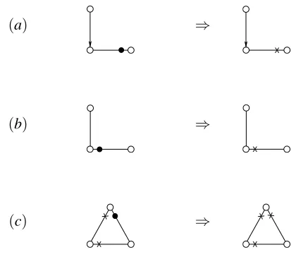
Figure 6: Three blocking rules from the labeling algorithm.

6.1 Labeling Algorithm

Let G= (N,A,L) be a CG. A labeled graph Gℓ= (N,A,Lℓ_{)is a graph obtained by ascribing a}

pair of labels to every line{a,b} ∈

L

. The labels on a line a−−−b correspond to endings of the line: one of them is associated with a and the other with b. We use two different kinds of labels: a blocking label denoted by a cross, ‘x’, and a label denoted by a dot, ‘•’, to be read as ‘free’. Thus, if the blocking label is associated with a on a−−−b then we will say that the line is blocked at a and write a−x−−b in Gℓ. On the other hand, the notation a−•−−_{b in G}ℓ_{will mean that the line is free at}

a. The intuition behind the terminology is as follows. A blocked ending at a node a will mean that the line cannot be replaced with an arrow directed to a, for otherwise we would get a graph outside H. A free ending at a will mean that no such conclusion has been derived so far.

Consequently, a labeled CG has three types of lines: two symmetric forms −x−−x and −•−−• _{, and}

an asymmetric form −x−−• . Let us emphasize that we only consider labeled graphs in which all lines

have both endings labeled. However, in our notation, labels need not be explicitly indicated. For instance, the notation a−−−x b in Gℓwill mean that either a−x−−x b in Gℓor a−•−−x b in Gℓ.

Algorithm 1 Pseudo-code for theLabelingAlgorithm(G). 1: input a CG G= (N,A,L)

2: put i=0

3: initialize Gℓ_i= (N,A,Lℓ_{)by replacing every line a−−−b in G by a−•−−• b in G}ℓ

i 4: while at least one forbidden configuration is present in Gℓ_i do

5: i=i+1

6: Gℓ_i=modify Gℓ_i−1by applying one of the following rules (see also Figure 6): (a) if a−→b−−−• _{c in G}ℓ

i−1and a and c are not adjacent then b−−−x c in Gℓi (b) if a−−−b−•−−c in Gℓ_i−1and a and c are not adjacent then b−x−−_{c in G}ℓ i (c) if a−−−x b−−−x c−•−−a in Gℓ_i−1 then c−x−−a in Gℓ i 7: end while

8: return Gℓ=Gℓ_i

The point is that the result of the labelling algorithm is invariant with respect to the order in which the blocking rules are applied.

Proposition 18 For any CG G, the labeled graph Gℓ=LabelingAlgorithm(G) is unique. This means that the output of the labeling algorithm does not depend on the ordering in which the three blocking rules are applied.

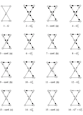
The proof can be found in the Appendix. In the rest of the paper, Gℓ will always denote the labeled version of G resulting from the application of Algorithm 1. An example of application of the labeling algorithm is given in Figure 7.

Note that Algorithm 1 is specified so that just one single label is changed in one iteration. This is useful in the proofs of the results of this section, but may be inefficient in practice. A more efficient implementation of the procedure can be achieved by applying the rules (a) and (b) first in a multi-step, and then only applying the rule (c) iteratively. This follows from Proposition 18 and the fact that the application of the rules (a) and (b) does not depend on the result of previous iterations of Algorithm 1.

6.2 Directing Algorithm

The directing algorithm, described in Algorithm 2, is the second building block of the deflagging procedure. It replaces some (labeled) lines with arrows in order to possibly reduce the number of flags in the original CG. More precisely, every line of the form a−x−−• _{b is replaced with the arrow}

a−→b and then the labels on other lines are removed.

Algorithm 2 Pseudo-code for theDirectingAlgorithm(Gℓ).

1: input a labeled CG Gℓ= (N,A,Lℓ₎

2: Gℓ_∗=modify Gℓby applying the following rule:

a−x−−• b in Gℓ ⇒ a−→b in Gℓ_∗ 3: G′= unlabeled version of Gℓ_∗

4: return G′

x

1 – G 2 – Gℓ₀ 3 –conf. (a) 4 – Gℓ₁

x x x x x x

x x

5 –conf. (a) 6 – Gℓ₂ 7 –conf. (b) 8 – Gℓ₃

x

x

x x

x x

x

x

x _x

x

x x

x x x

9 –conf. (b) 10 – Gℓ₄ 11 –conf. (b) 12 – Gℓ₅

x

x x

x x

x x

x x

x

x x

x x x

x x

x

x x

x x

x x

13 –conf. (c) 14 – Gℓ₆ 15 –conf. (c) 16 – Gℓ=Gℓ₇

Theorem 19 Let G be a CG, Gℓdenote the labeled graph obtained from G by Algorithm 1, and G′ the graph resulting from Gℓby Algorithm 2. Then G′is a CG which is triplex equivalent to G.

The proof is relatively long and we have placed it in the Appendix. Clearly, one has G≥G′ and, hence,

G

G

′ _{for the respective equivalence classes. Moreover, one has G6=G}′ _{unless no}

line is replaced with an arrow in the directing phase. An example of the application of the directing algorithm will be shown in the next section.

6.3 Overall Procedure

The application of the above algorithms to a CG G produces a graph G′in the same AMP equiva-lence class such that G≥G′. However, G′ still need not be a maximally deflagged graph and one can then apply the same procedure to G′. In Algorithm 3, we provide the pseudo-code of the over-all deflagging procedure which consists in repeated application of both algorithms until no line is replaced with an arrow during the directing phase. Its result will be denoted byG.b

Algorithm 3 Pseudo-code for theDeflaggingProcedure(G). 1: input G= (N,A,L)

2: j=0

3: initializeGbj=G 4: repeat

5: j=j+1

6: Gbℓ_j−1=LabelingAlgorithm(Gjb −1)

7: Gbj=DirectingAlgorithm(Gbℓj−1)

8: untilGbjis equal toGbj−1 9: returnGb=Gbj

Since G has a finite number of lines, the procedure will return a result in finitely many steps. An example of the application of the deflagging algorithm is given in Figure 8. Note that, in this example,G is already the largest deflagged graph from Figure 4; however, this is not true in general.b

x x x

x x

x

x

x x

G=Gb0 Gbℓ0 Gb1 Gbℓ1 Gb2 Gbℓ2 Gb=Gb3

Figure 8: An example of the application of the deflagging procedure, where G is the top left graph in Figure 4. Note that the first application of the labeling algorithm, to obtain Gℓ₀ from Gℓ, is detailed in Figure 7.

We are to show thatG is a deflagged graph, that is,b G inb

H

↓_where

_H

↓_{is the class of deflagged}

directing algorithm does not direct any line if applied to the labeled version ofG. This means, everyb line inGbℓis either of the type −•−−• _{or of the type} −x−−x .

Proposition 20 Let G be a CG such that there is no line of asymmetric form −x−−• _{in its labeled}

version Gℓ. Then, every line a−−−b in G such that a−x−−x b in Gℓis a line in every CG F which is

triplex equivalent to G.

The proof is again postponed to the Appendix. Proposition 20 is not valid if the assumption on G is omitted. A counterexample is given in Figure 8 where G=Gb0and F =G. A consequence ofb Proposition 20 is that every flag inG is an essential flag.b

Corollary 21 Given a CG G, the graph Gb=DeflaggingProcedure(G) is a deflagged graph, formallyG inb

H

↓.

Proof By Theorem 19, G belongs to the same AMP equivalence classb Has G. Owing to Propo-sition 8, we need to show that if a−→b−−−d is a flag in G then it is an essential flag. By theb blocking rule (a) a−→b−−−d inG implies ab −→b−−−x d inGbℓ. Since there are no lines of the form −•−−x inGbℓ, it necessitates a−→b−x−−x d inGbℓ. It follows from Proposition 20 that b−−−d in H for every H∈H. As a−→b−−−d has to correspond to a triplex in H, one can conclude that a−→b−−−d in H.

Note that the arguments in the proof above actually imply that a simple sufficient condition for a CG to be deflagged is that its labelled version has no line of asymmetric form.

7. Conclusions

This paper is devoted to the problem of choosing a graphical representative of the statistical model ascribed to a CG under AMP interpretation. As a matter of fact, any CG from the respective AMP Markov equivalence class provides a graphical representative of the corresponding model. However, a representative only makes sense if it complies with some properties that uniquely identify it within each class. Furthermore, in the framework of structural learning, the usefulness of a graphical representative is related to the availability of procedures which can be practically dealt with. That means, for instance, that an implementable construction procedure to obtain the representative (on the basis of any other graph in the Markov equivalence class) should be at our disposal.

Nevertheless, from the point of view of interpretation, a representative should be chosen on the basis of the information carried with respect to the corresponding statistical model. Hereafter, we address the issue of the information contained in the largest deflagged graph, which is the represen-tative for an AMP chain graph model we have proposed.

there are no essential flags inH. In this case, the class of deflagged graphs

H

↓_{is just the class of}

CGs without flags inH. Conversely, if there exists some essential flag in

H

↓then one can conclude that there is no CG inHfor which the two Markov properties coincide. Because deflagged graphs only contain essential flags, they eliminate the ambiguity resulting from the non-unique graphical representation of triplexes, and allow an immediate comparison with the LWF case.

The above reasons justify our restriction to the class of deflagged graphs. Now we justify the choice of the largest deflagged graph in

H

↓. If

H

↓ contains no flags then H↓ is the largest CG without flags in H. Thus, if Hcontains an undirected graph then the largest deflagged graph H↓ coincides with that undirected graph. Analogously, ifHcontains an acyclic directed graph D then H↓coincides with the essential graph D∗for D (Andersson et al., 1997; Studen´y, 2004; Roverato, 2005). We remark that the AMP essential graph H∗ proposed by Andersson et al. (2001) is a de-flagged graph (see Andersson and Perlman, 2006, Lemma 3.2(a) ) so that H∗≤H↓. Nevertheless, in general, the largest deflagged graph H↓is different from the AMP essential graph H∗: for instance, ifHcontains an undirected graph then H∗may even have some arrows (see Andersson et al., 2001, Figure 14).

Another issue related to the problem of representative choice is the topic of causal discovery in CGs (see Section 11.2 of Lauritzen, 2001). This is a controversial topic (see Section 3 of Dawid, 2002, for more discussion). The disputable question is whether one can identify some causal rela-tionships between variables on the basis of data. Nevertheless, what we think that what is generally accepted in the field of causal discovery is the following proposition:

If data are “generated” from a distribution which is “faithful” with respect to a CG and if an arrow a−→b is not invariant across the respective Markov equivalence class, then one cannot reveal possible causal relationship from a to b on basis of data.

In short, one cannot make causal discovery between a and b if there is an undirected edge between a and b in at least one of the chain graphs from the Markov equivalence class, or if there are two chain graphs such that a−→b in the one of them first and b−→a in the latter one. On the other hand, if an arrow a−→b is invariant across the respective Markov equivalence class then causal discovery could be possible. Consequently, from the point of view of causal discovery in chain graphs, a good representative of a Markov equivalence class should indicate that the corresponding edge is not an invariant arrow by the presence of a line. Standard representatives in the LWF case, such as the largest CGs (Studen´y, 1997), the essential graphs for acyclic directed graphs (Andersson et al., 1997), and the

B

-essential graphs (Roverato and La Rocca, 2006), are fully informative from this point of view because they have the largest number of lines and, furthermore, they contain an arrow if and only if it is invariant. As the examples in Figures 2 and 4 show, a CG with this property may not exist in an AMP equivalence class and therefore both the AMP essential graph and the largest deflagged graph may contain some arrows that are not invariant. However, the largest deflagged graph is more informative than the AMP essential graph because it is a larger chain graph and, therefore, it has more lines.

The results of the paper also lead to some natural open problems. For instance, we would like to know whether the converse of Proposition 20 is valid. More specifically, does the deflagging procedure identify all essential lines inHas double-blocked lines? Further conjecture is that the AMP essential graph is obtained if the deflagging procedure is applied to the largest deflagged graph. Another issue is as follows. We know that both LWF and AMP Markov equivalence are associated to Markov properties for CGs. Is there any Markov property for CGs which gives rise to the strong equivalence of CGs?

Acknowledgements

We are indebted to Nanny Wermuth who invited both of us to a workshop held in Wiesbaden in September 2002. We started there a discussion, which resulted in this paper. We also thank Michael Perlman for useful comments during the Barcelona meeting in 2004 and the anonymous referees for useful suggestions. Financial support to the fist author has been provided by Miur, PRIN03 and PRIN05 n. 134079. The research of the second author has been supported by GA ˇCR n. 201/04/0393.

Appendix A. Proofs

Proof of Proposition 12

Throughout the proof we assume that G and H are strongly equivalent CGs. Let G∪H and G∨H denote the graphs introduced in Lemma 11. We start with an auxiliary observation.

Fact 1 Let d0−→d1be a cyclic arrow in G∪H andρ: d0,d1, . . . ,dm≡d0, m≥3 a semi-directed cycle in G∪H containing it which cannot be shortened (to a semi-directed cycle in G∪H containing d0−→d1of the length l<m). Then d2−→d1in one of the graphs G and H while d0−→d2in the other graph.

Proof Since G is a CG, there exist 2≤j≤m with dj−1←−djin G and the same conclusion holds for H. Let us put

s=min{2≤ j≤m ; dj−1←−djeither in G or in H}.

Let us, without loss of generality, assume that ds−1←−dsin G. Then d0, . . . ,ds−1is a descending path G. Moreover, observe that d1, . . . ,dsis necessarily a descending path in the other graph, namely in H. This implies s<m for otherwiseρis a semi-directed cycle in a CG H.

The next step is to verify that [ds−2,ds]is an edge in G∪H. This is because otherwise ds−→ ds−1←−ds−2is an immorality in G or ds−→ds−1−−−ds−2is a flag in G, which, by strong equiv-alence of G and H, implies that ds−→ds−1 in H and this contradicts the assumption that ρis a semi-directed cycle in G∪H.

Since H is a CG and ds−2,ds−1,ds a descending path in H, one has either ds←− ds−2 or ds−−−ds−2in H, and, therefore, in G∪H.

Fact 2 There is no cyclic arrow a−→c in G∪H which belongs either to an immorality a−→c←− b or to a flag a−→c−−−b in G∪H.

Proof For a contradiction, suppose that at least one such cyclic arrow exists. Choose a semi-directed cycle ρ: d0,d1, . . . ,dm≡d0, m≥3 in G∪H of shortest possible length among all semi-directed cycles containing an arrow of this kind. Assume that d0=a−→c=d1is that arrow in G∪H and, using Fact 1, observe that d2−→d1in one of the graph, say in G, while d0−→d2in the other graph H.

Consider the induced subgraph over{a,c,b}mentioned in the formulation of Fact 2. As[a,b]is not an edge in G∪H whereas[d0,d2] = [a,d2]is an edge in H, one has d26=b. Observe that c←−b or c−−−b in G. Indeed, otherwise c−→b in G implies¬(c−→b in H)by the assumption of Fact 2, and H has either an immorality a−→c←−b or a flag a−→c−−−b. By strong equivalence of G and H, G has the same induced subgraph for{a,c,b}, which contradicts the fact c−→b in G. By interchange of G and H derive that c←−b or c−−−b in H as well.

This allows one to see that[b,d2]is an edge in G∪H as otherwise the induced subgraph of G for{d2,d1=c,b}having d2−→d1coincides, by strong equivalence of G and H, with the subgraph of H and the conclusion d2−→d1 in H contradicts the assumption thatρis a semi-directed cycle in G∪H. Since b,c,d2is a descending path in H one has either b−→d2or b−−−d2in H.

Thus, H has either an immorality d0−→d2 ←−b or a flag d0−→ d2−−−b. Since G and H are strongly equivalent, G has the same induced subgraph for{d0,d2,b}. Of course, the same conclusion holds for G∪H and d0−→d2is an arrow in G∪H belonging to a triplex.

Hence, it is impossible that m>3 as otherwiseρcan be shortened to d0,d2, . . . ,dm=d0by a cyclic arrow d0−→d2 of the considered type which contradicts its definition. However, if m=3 then the fact d3≡d0−→d2in G∪H contradicts the assumption thatρis a semi-directed cycle in G∪H.

Observe easily by contradiction that if G and H are strongly equivalent then

[d] if a−→c both in G and in H then an induced subgraph a−→c−→b occurs in H iff it occurs in G.

This observation is used in the proof of the following fact and also later.

Fact 3 There is no cyclic arrow c−→b in G∪H which belongs to an induced subgraph a−→ c−→b in G∪H.

Proof For a contradiction, suppose that such an arrow exists. Choose a semi-directed cycle

ρ: d0,d1, . . . ,dm≡d0, m≥3 in G∪H of shortest possible length among all semi-directed cycles containing an arrow of this kind. More specifically, assume that d0=c−→b=d1in G∪H. By Fact 1 observe that one can assume d2−→d1in G and d0−→d2in H. One has either d2←−d1or d2−−−d1in H for otherwise d2−→d1in G∪H contradicts the assumption thatρis a semi-directed cycle. As a−→c in H whereas d2←−d0=c in H, one has a6=d2.

Thus, H has an induced subgraph a−→c=d0−→d2, which implies, by the condition [d] men-tioned above Fact 3, that G has the same induced subgraph. In particular, G∪H has this induced subgraph as well. Thus, necessarily m≤3 for otherwiseρcan be shortened in G∪H by d0−→d2 to get a shorter cycle of the required type. If m=3 then d3=d0−→d2in G∪H implies a contra-dictory conclusion thatρis not a semi-directed cycle in G∪H.

Now, the proof of Proposition 12 follows directly from Lemma 11 and Facts 2 and 3. Since G and H are strongly equivalent an immorality or a flag in G occurs also in H and, therefore, in G∪H. By Fact 2 it is preserved in G∨H. Conversely, if a−→c←−b is an immorality in G∨H then it is also in G. If a−→c−−−b is a flag in G∨H then a−→c both in G and in H. The option c←−b in one of the graphs G and H is excluded because then the graph has an immorality a−→c←−b, which is saved in G∨H. If c−→b in both graphs then G∪H has an induced subgraph a−→c−→b. By Fact 3 the arrow c−→b remains in G∨H which contradicts the assumption. Thus, c−−−b either in G or in H and this implies, by their strong equivalence, that the flag a−→c−−−b is in G.

Proof of Proposition 15

This proposition is analogous to the result on LWF equivalence and feasible merging given in The-orem 8 of Roverato (2005). It says this:

Given a CG G and a meta-arrow U⇉L in G, the conditions (i) and (ii) from Definition 3 form together a necessary and sufficient condition for the graph G′obtained by merging U and L to be a CG which is complex equivalent to G.

In fact, we utilize this result in our proof of Proposition 15. Recall that the condition [i] from Definition 14 is identical to the condition (i) from Definition 3 and the condition [ii] from Definition 14 is stronger than (ii) from Definition 3.

Proof First, we are going to verify the necessity of the conditions [i]-[iii]. Since strong equivalence of CGs implies their complex equivalence the necessity of conditions (i)-(ii) follows from Theorem 8 in Roverato (2005). The conditions [i] and (i) are identical, but [ii] is stronger than (ii). Indeed, [ii] requires equality of sets pa_G(L)\U and pa_G(b) for every b∈K whereas (ii) only requires pa_G(L)\U⊆pa_G(b).

Thus, to verify [ii] it suffices to show

• ∀b∈K pa_G(b)⊆pa_G(L)\U .

Suppose for contradiction that b∈K and a∈ pa_G(b)exists with a6∈pa_G(L)\U . Then d∈L exists such that b−→d in G. Of course, a6=d and, since G is a CG, the options a←−d and a−−−d in G cannot occur. The option a−→d is excluded by the assumption a6∈ pa_G(L)\U . If[a,d]is not an edge in G then G has an induced subgraph a−→b−→d while G′ has a flag a−→b−−−d which contradicts the assumption that they are strongly equivalent.

The next step is to verify the necessity of the condition

[iii] for every de ∈L one has pa_G(L)⊆pa_G(d),

• b∈U , that is, b∈K.

Then there exists g∈L with b−→g in G. If g6=d then one can consider a path b−→ g−−−. . . −−−d in G and its shorteningρwhich cannot be shortened any more. If[b,d]is not an edge in G then G has a flag b−→e−−−f composed of nodes ofρ. This contradicts the assumption that G and G′are strongly equivalent since one has b−−−e in G′by definition of merging. Thus,[b,d]is an edge and b−→d in G since G is a CG.

• b∈ pa_G(L)\U .

Observe that a∈K exists by Definition 1 and b−→a follows from (ii). Moreover, one has a−→d in G by the previous case. If[b,d]is not an edge then G has an induced subgraph b−→a−→d while G′ has a flag b−→a−−−d which contradicts the assumption that they are strongly equivalent. Thus,[b,d]is an edge, namely b−→d in G because G is a CG.

This concludes the proof of the necessity of conditions [i]-[iii].

Second, we prove the sufficiency of those conditions. Since they imply the conditions (i)-(ii) from Definition 3, it follows from Theorem 8 in Roverato (2005) that G′is a CG which is complex equivalent to G but strictly larger. In particular, G and G′have the same immoralities and, to show that they are strongly equivalent, it suffices to verify that they have identical flags.

If a−→b−−−d is a flag in G then we are to show that it is a flag in G′. The only option which avoids the desired conclusion is a∈U and b∈L. However, then d∈L and by [iii] observe a−→d in G which contradicts the assumption.

If a−→b−−−d is a flag in G′ then the fact G′≥G implies a−→b in G and the only option which avoids the desired conclusion that a−→b−−−d is a flag in G is that[b,d]was modified. There are basically two cases.

• If b∈L and d∈U then a−→b←−d is an immorality in G and, because of complex equiv-alence of graphs, also in G′. This contradicts the assumption.

• If b∈U and d ∈L then observe b∈K and by [ii] a∈ pa_G(b)⊆ pa_G(L)\U . By [iii] get a∈pa_G(d)which contradicts the assumption.

Thus, the sufficiency proof is finished.

Proof of Proposition 16

Basic observation which is needed is as follows.

Fact 4 Let E,F,G be CGs over N with the same underlying graph such that E ≥F≥G and the following condition holds for any c∈N:

[e] if there exists a∈N with a−−−c in E and a−→c in F then for every b∈N with c−−−b in F one has c−−−b in G.

Note that the conclusion of Fact 4 need not be valid if the condition [e] is omitted: consider N={a,b,c}, E an undirected graph with a−−−c−−−b, F a CG with a−→c−−−b and G a directed graph with a−→c−→b.

Proof We can show that F is strongly equivalent to E. If a−→c←−b is an immorality in E then E≥F implies that it is an immorality in F. Conversely, if a−→c←−b is an immorality in F then F≥G implies that it is an immorality in G and, therefore, in E.

If a−→c−−−b is a flag in E, then it is a flag in G which implies c−−−b in F by F≥G. Since a−→c in F by E≥F the graph F has a flag a−→c−−−b.

If a−→c−−−b is a flag in F, then F≥G implies a−→c in G. We first verify a−→c in E by excluding two other variants of the edge[a,e]in E. Since E≥F the case a←−c in E is excluded. The case a−−−c in E is also excluded, this time owing to the condition [e] from the assumption of Fact 4. Indeed, [e] says c−−−b in G, which implies that a−→c−−−b is a flag in G and, therefore, in E, which contradicts the assumption a−−−c in E. Thus, a−→c in E and the aim is to show c−−−b in G. It can be shown by contradiction.

• If c←−b in G then a−→c←−b is an immorality in G and, therefore, in E, which implies, by E≥F, a contradictory conclusion c←−b in F.

• If c−→b in G then a−→c−→b is an induced subgraph in G. By the condition [d] mentioned above Fact 3 applied to G and E, it is also an induced subgraph in E. The assumption E≥F then implies a contradictory conclusion c−→b in F.

Hence, a−→c−−−b is a flag in G, and therefore in E.

The main step is the following ‘sandwich lemma’.

Fact 5 Let G,E be strongly equivalent CGs, E ≥G, E6=G. Then there exists a CG F which is strongly equivalent to G and E, such that E≥F≥G and E is obtained from F by legal merging of components.

Note that the idea of the proof of this proposition is analogous to the proof of Theorem 7 in Roverato (2005).

Proof Since E≥G, every component in E is the union of components in G and the assumption E6=G implies that there exists a component C in E containing at least two components in G. As GCis a CG one can find a terminal component T in it. By the construction C\T6=/0and there is an arrow from C\T to T in G. Let us construct a hybrid graph F from E by replacement of all lines between C\T and T in E by arrows from C\T to T . Observe the following facts.

{a} F is a CG.

{b} E≥F≥G and F6=E.

The fact E≥F is evident. To see F≥G observe that if a−→b in F then either a−→b in E in which case E≥G implies a−→b in G, or a−−−b in E. In the latter case a∈C\T and b∈T which also implies, by the definition of T , that a−→b in G.

{c} C\T is a connected set in F and, therefore, it is a component in F.

Indeed, suppose for contradiction that distinct a,b∈C\T exist which are not connected by an undirected path in F_C\T=E_C\T. Since C is a connected set in E, one can construct a path

˜

a−→c1−−−. . . −−−cm←− ˜b, m≥1 in F with some c1, . . . ,cm∈T and ˜a,˜b∈C\T such that[a˜,˜b]is not an edge in F. This path has the same form in G and can be shortened to a complex in G. This complex is not in E which contradicts the assumption that E and G are strongly equivalent since strong equivalence implies complex equivalence.

{d} F is strongly equivalent to G and E.

This follows from Fact 4 owing to{a}and{b}. The condition [e] from Fact 4 holds because of the construction of F: if a−−−c in E and a−→c in F then c∈T and c−−−b in F implies b∈T for which reason c−−−b in G.

Now, the conclusion that E is made of F by legal merging of components is easy to see. The condi-tion{c}implies that both C\T and T are components in F and E is obtained from F by merging of the upper component U ≡C\T and the lower component L≡T . Since E and F are strongly equivalent is follows from Proposition 15 that the merging is legal.

Now, the proof of Proposition 16 is easy. The required sequence G=F1, . . . ,Fm=H, m≥1 can be constructed backwards by consecutive application of Fact 5 to G and E≡Fito get Fi−1=F until Fi−1is the graph G. Of course, one starts with Fm=H, where m−1 is the difference between the numbers of components of G and H.

Proof of Proposition 18

Assume for contradiction that two different orderings of applications of blocking rules leads to two different labeled graphs Gℓ(1) and Gℓ(2). Since they only differ in their labels, one can assume without loss of generality that Gℓ(1)has at least one blocked label that is ‘free’ in Gℓ(2). Let us fix a sequence of iterations G₀ℓ(1),G₁ℓ(1), . . . ,Gℓn(1)=Gℓ(1), n≥2 leading to Gℓ(1). Let Gℓ_i(1)be the first graph in this sequence which has a blocked label that is ‘free’ in Gℓ(2), say a−x−−d ∈Gℓ(1)

i and a−•−−d∈Gℓ(2). In particular, b−x−−c in Gℓ(1)

j for j<i implies b−x−−c in Gℓ(2). We now show that a−x−−d∈Gℓ(1)

i and a−•−−d in Gℓ(2) implies that Gℓ(2) has a forbidden configuration, which contradicts the assumption. There are three possible cases.

1. If a−x−−d in Gℓ(1)

i is blocked at a by the rule (a) then there exists a vertex b such that b−→ d−−−a is a flag in G (cf. Algorithm 1). In particular, b−→d−−−• _{a in G}ℓ(2)_{is a forbidden}

configuration in Gℓ(2). 2. If a−x−−d in Gℓ(1)