Distance Patterns in Structural Similarity
Thomas K¨ampke [email protected]
Forschungsinstitut f¨ur Anwendungsorientierte Wissensverarbeitung/n FAW/n Lise-Meitner-Str. 9
89081 Ulm, Germany
Editor: Peter Dayan
Abstract
Similarity of edge labeled graphs is considered in the sense of minimum squared distance between corresponding values. Vertex correspondences are established by isomorphisms if both graphs are of equal size and by subisomorphisms if one graph has fewer vertices than the other. Best fit isomorphisms and subisomorphisms amount to solutions of quadratic assignment problems and are computed exactly as well as approximately by minimum cost flow, linear assignment relaxations and related graph algorithms.
Keywords: assignment problem, best approximation, branch and bound, inexact graph matching,
model data base
1. Introduction
Structural similarity is involved in a variety of pattern recognition problems when considered from an abstract perspective. The abstraction refers to measurements and observations whose specifics are ignored. One class of such problems is encountered in image processing, where a set of features or objects with topological interrelations is detected in several scenes. Whenever these are presumed to be similar according to position, proximity or else, the degree of similarity is of interest.
Structures are represented throughout by labeled graphs such as image graphs. In image graphs, vertices represent image edges, corners or regions of interest such as regions of constant intensity or homogenous texture. Graph edges represent relations such as neighborhoods or concept hierarchies. Edge labels represent distances, degrees of association or else.
Structural similarity is considered as similarity between two labeled graphs. Typical roles of the two graphs are that of a model graph from a model data base or a prototype data base and that of an instance graph representing an ’as is’ structure which is encountered ’at run time’. The issue is then to determine the similarity between prototype and instance.
Similarity will be formulated as a best approximation problem. This involves minimization of squared distances which results in a quadratic assignment problem. The problem is approached by several algorithmic concepts including network algorithms with emphasis on linear assignment relaxations. Also, cost minimal flows of given strength will play a major role. The focus is on approximate algorithms for best graph approximation since the exact problem is NP-hard.
The remainder of this work is organized as follows. Section 2 introduces the best approxima-tion problem for edge-labeled graphs and reviews related work. Polynomial time approximaapproxima-tion algorithms are stated in Section 3. Since the best graph approximation problem contains subgraph isomorphism as a special case, no exact algorithm can be expected to run in polynomial worst case time. The approximations are consequently based on linear assignment problems since the original problem is a quadratic assignment problem. Approximations have interesting side features such as being suited for grid computations. Section 4 contains two sketches of approaches for exact algo-rithms for the best graph approximation problem. One is based on flows, the other on branch and bound.
Unless otherwise stated, all graphs considered are undirected which means that edges have no preferred directions. Moreover, the graphs are simple which means that there is at most one edge between any two vertices and there are no loops so that no edge begins and ends in the same vertex. The edge labels themselves must allow to be subtractable from each other but are otherwise uncon-strained. In particular, the edge labels themselves do not have to reflect any notion of similarity.
The 2-norm or Euclidean norm of any vector z= (z1, . . . ,zn) of real numbers zi is denoted by ||z||=||z||2=
q
z21+. . .+z2
n. The number of elements of a finite set A is denoted by|A|.
2. Problem and Related Work
A distance pattern is understood to be an undirected graph with edge labels. The graph vertices denote objects or states and the edge labels denote distances, transition times etc. Though it may take quite some effort to generate these graphs in applications, this effort is ignored here and two such graphs are assumed to be given.
2.1 Problem Formulation
The best approximation of a labeled graph by another labeled graph is defined by a subisomorphism of the vertex set of the first graph to the vertex set of the second graph. Thereby edge labels of the first graph are approximated by corresponding edge labels of the second graph as minimum sum of squared differences.
Formally, two undirected graphs with edge labelings are given by G1= (V1,E1)with l1: E1→IR and G2= (V2,E2)with l2: E2→IR. The first graph has n=|V1|vertices and the second graph has
m=|V2| vertices with n≤m. The best approximation of G1 by G2 is defined via an optimal
approximating subisomorphism
ϕ0=argmin
ϕ:V1→V2,ϕinvertible
s
∑
{vi,vj}∈E1
l1(vi,vj)−l2(ϕ(vi),ϕ(vj)) 2
.
The best approximation is given by the image of the first vertex setϕ0(V1)so thatϕ0(V1)⊆V2. The minimum value is called the distance of the best approximation.
The objective of best approximation can be considered as Frobenius distance when both graphs are complete. The edge labelings then denote distance matrices D1,D2with entries
D1(vi,vj) =
l1(vi,vj), for vi6=vj
0, for vi=vj D2(wi
,wj) =
l2(wi,wj), for wi6=wj
0, for wi=wj.
The best approximation objective can then be written as follows since counting over all edges amounts to counting twice over all vertex pairs. Pairs of identical vertices are negligible because they contribute value zero.
∑
{vi,vj}∈E1
l1(vi,vj)−l2(ϕ(vi),ϕ(vj)) 2
= 1
2v
∑
i,vj∈V1
D1(vi,vj)−D2(ϕ(vi),ϕ(vj)) 2
= 1
2||(D1(·,·))−(D2(ϕ(·),ϕ(·)))|| 2 F.
The Frobenius norm of any matrix is the square root of the sum of all squared entries (Golub and van Loan, 1985).
Distance matrices allow to consider the best approximation problem also for graphs which are not complete. Whenever one of the two given graphs is not complete, all missing edges are inserted. The complete graph is then labeled by the shortest path distances according to the original edge labeling. Original edge labels are preserved when these satisfy the triangle inequality. Original edge labels may be overwritten when these do not satisfy the triangle inequality.
The celebrated graph isomorphism problem is contained in the best approximation problem as
the following special case. Suppose H1 and H2 are two unlabeled graphs with same number of
vertices and arbitrary edge sets. Each graph is extended to the complete graph on its vertex set and receives the edge labels
li(e):=
1, if edge e belongs to original graph Hi
0, if edge e does not belong to original graph Hi,
i=1,2. These graphs are denoted G1 and G2respectively. The original graphs are isomorphic if
and only if the best approximation of G1by G2and the best approximation of G2by G1both have distance zero.
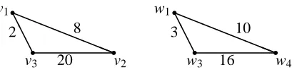
The most trivial case of the best approximation problem is given for the smaller graph being the smallest possible. This is a two vertex graph with one edge only. The single edge graph is best approximated by that edge from the larger graph whose label comes closest to the label of the single-edge graph. A non-trivial example of the best approximation problem is given in Figures 1 and 2.
Best graph approximation can be considered as search for a minimum weight clique of given size in a suitably defined graph, the association graph or correspondence graph. This relation is such that the given clique size equals the size of the smaller graph and that no larger cliques exist in the association graph. Mnemonically, best graph approximation can thus be remembered as search for a minimum weight clique of maximum size.
r
v3 rv2
r
v1
20
A A A
2aaaaaa
aa
8
r
w5 w4r
r
w1 rw3
r
w2
62
A A A
3
10
!!!! !!11!!
aaa
aaa10 aa
7 3
A A
A A
A A
9
16 Q Q Q Q Q
6
Figure 1: The left three vertex graph is best approximated by the triangle with edge labels 3,10,16
in the larger graph. The subisomorphism isϕ(v1) =w1,ϕ(v2) =w4andϕ(v3) =w3with
the two vertices w2 and w5being unattained. The graph isomorphism is given explicitly
in the next figure.
r
v3 rv2
r
v1
20
A A A
2aaaaaa
aa
8
r
w3 rw4
r
w1
16
A A A
3aaaaaa
aa
10
Figure 2: Original graph (left) and best approximating isomorphic substructure (right) for the situ-ation of Figure 1. The squared distance between the two graphs is(2−3)2+ (8−10)2+ (20−16)2=21.
cost of the edge between the vertices(vi,wj)and(vk,wl)is set equal to(D1(vi,vk)−D2(wj,wl))2. The meaning of selecting any vertex of the form(vi,wj)is that the original vertex vi is mapped to
the original vertex wj by a subisomorphism. These ”associations” motivate the name association
graph and the cost of a clique, which equals the cost sum over all edges between selected vertices, is the objective of graph approximation.
An alternative view of best graph approximation can be obtained from quadratic assignment problems such as the following
min
x x
TCx
such that n
∑
i=1xi j≤1 ∀j=1, . . . ,m
m
∑
j=1xi j=1 ∀i=1, . . . ,n
xi j∈ {0,1} ∀i,j.
The binary variable xi j attaining value one means that vertex vi is assigned to vertex wj and that variable attaining the value zero means that this assignment is not valid. The vector x has n·m
coordinates and C is an n·m×n·m matrix denoting the cost incurred by pairwise assignments;
r
(v1,w4)
r
(v1,w3)
r
(v1,w2)
r
(v1,w1)
r
(v2,w4)
r r r
(v2,w1)
r
(v3,w1)
r
(v3,w2)
r
(v3,w3)
r
(v3,w4)
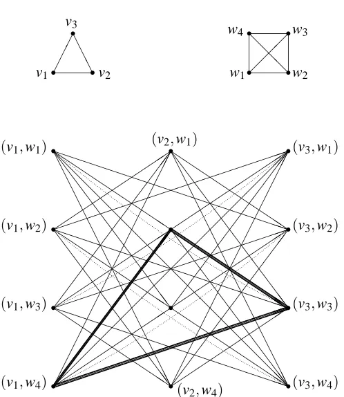
Q Q Q Q Q Q Q QQ PPP PPP PPP PPP PPPPP P Q Q Q Q Q Q Q QQ S S S S S S S S S S SS PPP PPP PPP PPP PPPPP P Q Q Q Q Q Q Q QQ S S S S S S S S S S SS A A A A A A A A A A A A A A A A AA PPP PPP PPP PPP PPPPP P @ @ @ @ @ @ @ @ @ @ @ @ @ @ @ @ @@ Q Q Q Q Q Q Q QQ Q Q Q Q Q Q Q QQ S S S S S S S S S S SS Q Q Q Q Q Q Q QQ S S S S S S S S S S SS A A A A A A A A A A A A A A A A AA QQ QQ QQ Q QQ QQ QQ QQ Q QQ r
v1 rv
2 r v3 A A
A w r
1 rw
2
r
w4 rw3
@ @
@
Figure 3: A ”small” graph and a ”large” graph (top) and their association graph (bottom). The indicated clique of the vertices(v1,w4),(v2,w2)and(v3,w3)denotes the subisomorphism ϕ(v1) =w4,ϕ(v2) =w2andϕ(v3) =w3.
computed as
C=
(D1(v1,v1)−D2(·,·))2 . . . (D1(v1,vn)−D2(·,·))2 ..
. ... ...
(D1(vn,v1)−D2(·,·))2 . . . (D1(vn,vn)−D2(·,·))2
where D2(·,·) is the m×m matrix of all distance values for the second graph and(c−M)2, the square of a constant c minus a matrix M, is understood as a matrix of the size of M with each element denoting the squared distance from the constant so that(c−M)2= ((c−m
ab)2)ab. The size of the cost matrix is unfortunately large as it already is a 15×15 matrix for the small graphs from Figure 1.
2.2 Related Work
problem also is NP-complete, see Garey and Johnson (1981, problem GT49). This problem allows edge removals only in order to find isomorphic subgraphs. Here, only vertex removals matter and edge removals are allowed only in so far as they are implied by vertex removals.
A widely used measure for so-called inexact graph matching is the edit distance between two unlabeled graphs. One graph is therefore modified by a minimum number of vertex insertions and deletions and by edge insertions and deletions. The concept in general as well as a particular focus on tree graphs is given in Wang et al. (1998). A simplification of the edit distance does not refer to the graphs themselves and isomorphism between them but to their degree histograms which are to be made equal by a minimum number of changes (Papadopoulos and Manolopoulos, 1999). The edit distance for subisomorphisms of labeled graphs is considered by Messmer and Bunke (1998a). Subisomorphism with vertices and edges both carrying labels is considered by Hlaoui and Wang (2002). Conflicts of tentatively assigning several vertices of the smaller graph to one vertex of the larger graph are resolved in a hierarchical manner. The method is reported to be well suited for small graphs. Best graph approximation in terms of matching problems is considered by Gold and Rangarajan (1996). There, the problem is extended to a sequence of continuous surrogate prob-lems. This leads to an iterative, matrix-based solution scheme which is controlled by a continuous parameter that intends to drive continuous relaxations to a discrete vertex assignment. While leav-ing slight uncertainties about the control of this parameter and while usleav-ing a linear instead of a quadratic distance between edge labels, the method makes, like the approaches given below, use of the assignment problem. A quite different, probabilistic approach which makes use of potential functions is given in Caetano et al. (2005).
Best graph approximation can be considered as ”dual” to joint edge and label construction. This construction was developed for trees by Desper and Vingron (2002). Only distance information is required in order to build one tree with edge weights so that the given distances are approxi-mated by path lengths between leaves of the tree. The construction is formulated as a least square approximation problem so that solution methods have a strong algebraic component.
Matching techniques for graphs whose vertices denote positions in space have been developed from the analogy of physical elasticity, compare Wiskott et al. (1997) and Wiskott and Malsburg (2002). In addition, the elasticity idea supports the generation of the model graph from examples. These physical methods are complemented by probabilistic methods for unlabeled graph subiso-morphisms by Bengoetxea (2002).
Motivated by graphs that describe the structure of SQL data bases, an interactive fixpoint al-gorithm for similarity computing has been proposed by Melnik et al. (2002). The method is based on the assumption that adjacent vertices are more similar than non-adjacent vertices. The quality of the matching result is measured by the number of human adjustment steps that are eventually needed. For a similar data base purpose, case-based reasoning, similarity of graphs with character-string labels has been considered (Champin and Solnon, 2003). Similarity is measured by weighted counts of identical labels with vertex correspondence being generated by a greedy algorithm. This algorithm maximizes the similarity score in each iteration.
the smaller graph is known to be contained in the larger graph, methods for PARTIAL DIGEST can help to identify the actual subgraph isomorphism.
Subgraph isomorphism for unlabeled graphs has been studied in Messmer and Bunke (1998b) motivated by symbol recognition problems. A polynomial time algorithm is given which requires preprocessing and exponential space in the worst case. Graph similarity has even been investigated for machine learning (Pope and Lowe, 1996). A quite sketchy outline of graph search methods over molecular graphs is presented in Shasha et al. (2002), while the perspective of distance methods for molecular similarity and superstructure retrieval is given in K¨ampke (2004).
3. Approximate Algorithms
The best approximation problem obviously is finite and, thus, can, in principle, be solved by enu-meration over all mnn! selections for admissible functionsϕ. Approximate algorithms of different types as well as a strategy for exact algorithms are given in the sequel. The present approximations mainly focus on linear assignment problems since the original problem is a quadratic assignment problem.
To illustrate the intuitive aim of best graph approximation, the squared approximation distance is rewritten for the special case of equally sized graphs. The best isomorphism then is a solution of the maximization problem
max
ϕ:V1→V2,ϕinvertible{v
∑
i,vj}∈E1D1(vi,vj)·D2(ϕ(vi),ϕ(vj)).
The sum can be considered as an inner product over edges. When all edges of the first graph are sorted increasingly then the maximization is obtained by an isomorphism that maintains monotonic-ity ”as far as possible”. This is motivated by the well known inner product maximization∑Ni=1aibπ(i)
problem over all permutationsπ. The solution is a permutation with bπ(1)≤. . .≤bπ(N)whenever
all coordinates of the first vector are sorted as a1≤. . .≤aN, compare with Hardy et al. (1948). A monotonicity preserving isomorphism does generally not exist for the edge labels.
3.1 Distance Lists
A heuristic procedure for best subgraph isomorphism can be devised on local, that is, vertex-oriented decisions. These are based on distance lists. The distance list of a vertex contains the labels of all edges that are incident with the vertex. Any distance list can also be considered as a vector. The distance list of a vertex v is denoted by distlist(v). A distance list in a complete graph with edge labels D(·,·) is given by distlist(v) = (D(v,vi))vi∈V−{v}. For the ease of comparability, all vertex
lists are sorted increasingly. Distance lists generalize vertex degrees since they count the ”ones” when unlabeled graphs receive the binary edge labeling as given above for the embedding of the graph isomorphism problem.
The distance lists for the three-vertex graph from Figure 1 are given by distlist(v1) = (2,8), distlist(v2) = (8,20)and distlist(v3) = (2,20). The five-vertex graph of the same figure has the dis-tance lists distlist(w1) = (3,3,7,10), distlist(w2) = (6,7,7,9), distlist(w3) = (3,6,8,16), distlist(w4) = (9,10,16,62)and distlist(w5) = (3,7,8,62).
distance lists have different numbers of coordinates, a proper selection is made from the larger distance list. In the foregoing example, selections of two out of the four coordinates from the distance lists of the five-vertex graph are made.
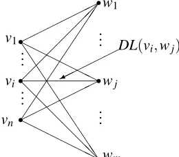
The approximation of a distance list by a selection from a larger distance list can be formulated as a weighted or cost minimal assignment problem. Therefore, two distance lists distlist(v) = (x1, . . . ,xn−1)and distlist(w) = (y1, . . . ,ym−1), n≤m, are endowed with a complete bipartite graph. Each coordinate receives one vertex and each coordinate of one distance list is connected by an edge to each coordinate of the other distance list. No two coordinates of the same list are connected. The edge connecting coordinates xi and yj is labeled by the squared difference of the list entries (xi−yj)2, compare with Figure 4.
r
xn−1 .. .
r
xi .. .
r
x1
rym−1
.. .
ry
j .. .
ry1
HH HH
HH J
J J
J J
J J
JJ
(xi−yj)2
@
@ @
@ @
@
HH HH
HH
Figure 4: Complete bipartite graph for two distance lists. The vertices correspond to the coordinates of the distance lists rather than to the vertices of the original graphs. Only one of the (n−1)·(m−1)edge labels is sketched.
Any approximation of the first distance list by the second distance list amounts to a selection
of n−1 distinct coordinates or indices from the second list. The approximation objective can be
formulated as a linear function of the edge labels
min 1≤j1<...<jn−1≤m−1
n−1
∑
i=1(xi−yji)
2 .
Alternatively, the best approximation problem for distance lists can be formulated as cost minimal perfect matching problem and as a cost minimal integral flow problem with flow value set to level
n−1, compare with Section 4.
The best approximation of a distance list distlist(v)by the distance list distlist(w) is denoted
as the projection pr(distlist(w), distlist(v)). The squared approximation error equals DL(v,w) =
distlist(vi) distlist(wj) pr(distlist(wj), DL(vi,wj) distlist(vi))
(2,8) (3,3,7,10) (3,7) (2−3)2+ (8−7)2=2 (2,8) (6,7,9,10) (6,7)or(6,9) (2−6)2+ (8−7)2=17 i=1 (2,8) (3,6,11,16) (3,6) (2−3)2+ (8−6)2=5
(2,8) (9,10,16,62) (9,10) (2−9)2+ (8−10)2=53 (2,8) (3,10,11,62) (3,10) (2−3)2+ (8−10)2=5 (8,20) (3,3,7,10) (7,10) (8−7)2+ (20−10)2=101 (8,20) (6,7,9,10) (7,10)or(9,10) (8−7)2+ (20−10)2=101 i=2 (8,20) (3,6,11,16) (6,16) (8−6)2+ (20−16)2=20
(8,20) (9,10,16,62) (9,16) (8−9)2+ (20−16)2=17 (8,20) (3,10,11,62) (10,11) (8−10)2+ (20−11)2=85 (2,20) (3,3,7,10) (3,10) (2−3)2+ (20−10)2=101 (2,20) (6,7,9,10) (6,10) (2−6)2+ (20−10)2=116 i=3 (2,20) (3,6,10,16) (3,16) (2−3)2+ (20−16)2=17
(2,20) (9,10,16,62) (9,16) (2−9)2+ (20−16)2=65 (2,20) (3,10,11,62) (3,10) (2−3)2+ (20−10)2=101 3.2 Best Approximations by Distance Lists
The idea of cost minimal assignments can be carried over from distance lists of single vertices to the whole graph. This results in an efficient heuristic algorithm for best graph approximation. Again, the approximation problem is formulated as cost minimal assignment problem over a complete bipartite graph. One set of vertices corresponds to the smaller graph and the other to the larger graph. The edges are labeled by the errors of best distance list approximations. The general situation is sketched in Figure 5.
r
vn .. .
r
vi .. .
r
v1
rwm
.. .
rw
j .. .
rw1
HH HH
HH J
J J
J J
J J
JJ
DL(vi,wj)
@
@ @
@ @
@
HH HH
HH
Figure 5: Complete bipartite graph for a heuristic solution of best graph approximation. The edge labels refer to best approximations of distance lists.
ApproxDistList
1. Input complete labeled graphs G1,G2with|V1| ≤ |V2|.
Initialization. Computation of distance list errors DL(v,w) for all v∈V1, w∈V2. A=V , B=W .
2. While A6=/0do
(a) Computation of W(v) =argminw∈BDL(v,w)and level(v,B) =DL(v,W(v))and for all v∈A.
(b) Selection of v0=argminv∈Alevel(v,B). (c) ϕ(v0) =w(v0)with w(v0)∈W(v0). (d) A=A− {v0}.
(e) B=B− {ϕ(v0)}.
3. Output subisomorphismϕ(·)on V1.
The level computations in step 2(a) determine the best fit decision that can be made without taking back prior decisions. The sets W(v)indicate all vertices from the second graph that attain the minimum. Ties for selections in step 2(b) as well as for selections from the set W(v0)in step 2(c) are broken arbitrarily. While the sets A and B of unassigned vertices decrease along the iterations of the algorithm, the distance lists to consider become fewer but not smaller. Thus, the edge labels DL(v,w)do not have to be updated along the iterations.
The greedy procedure applied to the graphs of Figure 1 can be traced with the data from the table of Section 3.1. The resulting subisomorphism is given by selecting the minima for each vertex from the smaller graph. This is exactly the solution indicated by Figure 2.
The foregoing algorithm need not solve the cost minimum assignment problem exactly. An optimal solution of this problem (which still need not lead to the best graph approximation since the assignment problem is only an approximative encoding for best graph approximation problem) can be found by any weighted assignment algorithm for bipartite graphs. These algorithms are typically based on transformations to cost minimum flow problems. Therefore, all vertices of the smaller graph are connected to an extra source vertex and all vertices of the larger graph are connected to an extra sink vertex. All the extra edges receive a unit capacity on the flow. All edges become oriented edges or arcs as indicated in the flow network in Figure 6.
Among the cost minimal flows of strength n there is one with all integer values. This flow amounts to a cost minimal assignment of all vertices from the smaller graph. The out of kilter algorithm allows to compute the desired cost minimum flow, see Ahuja et al. (1993).
A different solution for cost minimal assignment problems can be obtained from straightforward transformations to cost minimal perfect matching problems by introducing additional vertices for the smaller graph. Both sets of the vertex partition then have the same size. All dummy vertices for the smaller graph are connected to all vertices from the larger graph by edges with zero cost. A matching is a set of edges such that any two edges do not have a common vertex. A matching is perfect if each vertex of the graph is covered by an edge.
r
source
r
vn .. .
r
vi .. .
r
v1
r
wm .. .
r
wj .. .
r
w1
rsink
* cap=1
-cap=1 HH
HH HHj cap=1
*
HH HH
HHj J
J J
J J
J J
JJ^
-DL(vi,wj)
@
@ @
@ @
@ R
*
HH HH
HHj @
@ @
@ @
@ R cap=1
-cap=1
cap=1
Figure 6: Flow network for a distance label heuristic. The edges that are incident either to the source or the sink carry capacities but no cost coefficients while the edges with cost coefficients do not carry capacities.
3.3 Direct Methods
Direct methods for graph approximation will use the original edge labels and the unaltered best approximation errors for all fitting assessments.
3.3.1 SEQUENTIAL ASSIGNMENTS
A subisomorphism can be constructed by sequentially assigning vertices from the smaller graph to the larger graph so that the sum of squared label distances over all new edge pairs is minimal. The first assignment may stem from two best matching edges. No assignment is ever revised by the following procedure.
SeqAssign
1. Input complete labeled graphs G1,G2with|V1| ≤ |V2|.
Initialization. Computation of(e0,f0) =argmine∈E1,f∈E2(D1(e)−D2(f))
2. Selection of one vertex v1of the two vertices incident with e0. Selection of one vertex w1of the two vertices incident with f0. ϕ(v1) =w1.
Labeling all other vertices from V1by v2, . . . ,vn. B=V2− {ϕ(v1)}.
2. For i=2, . . . ,n do
(a) Computation of w0=argminw∈B∑ij−1=1(D1(vj,vi)−D2(ϕ(vj),w)2. (b) ϕ(vi) =w0.
(c) B=B− {ϕ(vi)}.
3.3.2 IMPROVEMENTS
Whenever a subisomorphism is not optimal or not known to be optimal, improvements can be aimed at by swapping two vertex assignments or by swapping an assigned with an unassigned vertex. Swaps of both types can easily be evaluated.
For notational ease the vertices are numbered such thatϕ(vk) =wk, k=1, . . . ,n, for some given subisomorphismϕ: V1→V2. First, two vertices vi,vj, 1≤i6= j≤n are considered for swapping their assignments while all other assignments are preserved.
ϕ0(v k) =
wj if k=i wi if k= j wk if k6=i,j.
The new subisomorphism leads to a smaller approximation error if and only if
n
∑
k=1,k6=i,j
l1(vi,vk)−l1(vj,vk)
·l2(wj,wk)−l2(wi,wk)
>0.
This condition being true is denoted byImp(i,j) =true. Second, one vertex vi, 1≤i≤n is con-sidered for changing its assignment to an unassigned vertex w0∈V2−ϕ(V1), that is, the present subisomorphism is compared to the new subisomorphism
ϕ0(v k) =
w0 if k=i wk if k6=i.
The new subisomorphism leads to a smaller approximation error if and only if
n
∑
k=1,k6=il22(wi,wk)−l22(w0,wk)>2 n
∑
k=1,k6=il1(vi,vk)·
l2(wi,wk)−l2(w0,wk)
.
This condition being true is denoted byImp(i,w0) = true. The improvement conditions results in the following procedure.
Imp
1. Input complete labeled graphs G1, G2.
Subisomorphismϕ: V1→V2withϕ(vk) =wk, k=1, . . . ,n. 2. WhileImp(i,j) =trueorImp(i,w0) = true for somew0do
(a) IfImp(i,j) =truethenϕ(vi) =wj andϕ(vj) =wi elseϕ(vi) =w0
(b) Vertex relabeling such thatϕ(vk) =wk, k=1, . . . ,n.
3. Output swap-improved subisomorphismϕ: V1→V2.
3.4 Relaxation Method
The previous methods can all be considered as primally feasible which means that all assignments actually are subisomorphisms though not necessarily optimal. The subisomorphism constraint may tentatively be relaxed in analogy to so-called dual optimization techniques. Starting from some promising structure, a sequence of changes will be made that eventually attain feasibility and that tend to incur as little additional cost as possible per step.
3.4.1 INITIALSTRUCTURE
A promising initial structure is constructible by enumerating the first vertex set. Each vertex from that set is paired with all vertices from the second vertex set which amounts to considering their common vertices in the association graph. The label sum of all edges which emanate from each of these common vertices is minimized under the choice of the second vertex. This can be expressed as the following nested minimization:
µ(i) =argminj=1,...,m n
∑
k=1,k6=imin l=1,...,m
D1(vi,vk)−D2(wj,wl) 2
.
This minimization implies a function from the first vertex set into the second vertex set by vi7→wµ(i). The inner minimizations are independent of each other and, thus, may lead to
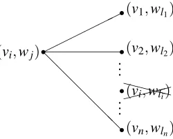
overas-signments which means that the same index l is attained as minimum for different outer indices. The analogue is true for the outer minimization. The presence of overassignments implies that the overall function is not a subisomorphism. However, the independence of the minimizations makes them easy to compute and the resulting cost value provides a lower bound for the cost of best graph approximation. The edges for summation in one minimization of the initial relaxation are sketched in Figure 7. It is worth noticing that the minimization for the initial structure may lead to even
r
(vi,wj)
r(vn,wl n)
.. . .. .
r(v2,wl2) r(v1,wl1)
r(v
i,wli)
XXXX
@ @
@ @
@ @
Figure 7: Vertices and edges of the association graph that are considered while computing the value µ(i)for the initial structure of the relaxation method.
smaller objective values than the distance lists.
3.4.2 IMPROVEMENT
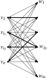
The edges for the wave front computations are directed. All edges of the current structure are oriented as backward edges from the second vertex set to the first vertex set and all other edges are oriented as forward edges from the first to the second vertex set, see Figure 8. Not all edge labels are initially known in quite a contrast to the ordinary dual method for assignment problems. Actually, node potentials will be computed according to edge transitions rather than by explicitly given edge labels.
r
vn
r
vi2
r
vi1
r
v1
rwm
r rwj
0
r r
rw1
HHH H H H Y H H H H H H H H H H H H HH HH HHj * @ @ @ @ @ @ R HH HH HHj * J J J J J J J JJ^ @ @ @ @ @ @ R * A A A A A A A A A A AAU J J J J J J J JJ^ @ @ @ @ @ @ R HH HH HHj *
Figure 8: Forward edges (thin) and four backward edges (bold) for the wave front computations to
resolve the double assignment of vertex wj0. The wave front begins in that vertex and
ends in a suitable vertex from the second set from which no edge leads back into the first set.
The relaxation method assigns tentative and permanent labels to graph nodes in analogy to the Dijkstra algorithm. The labels are potentials which equal the cost of functions from the first vertex set or a subset thereof into the second vertex set. Such functions need not be one-to-one. For-mally, the potential of a functionϕis computable as cost(ϕ) =∑v∈dom(ϕ)∑v0∈dom(ϕ)−{v}(D1(v,v0)− D2(ϕ(v),ϕ(v0)))2, where dom(ϕ)denotes the domain of functionϕ. Whenever a function is altered by deleting an assignment like v47→w3 it is denoted byϕ−(v47→w3), when then the assignment
v47→w8 is inserted, the function is denoted byϕ−(v47→w3) + (v47→w8) etc. Backward edges
amount to deleting assignments and forward edges amount to inserting assignments.
NoPo
1. Input Structureϕ, overassigned vertex w0∈V2.
Initialization L=V1∪V2− {w0}, m(l) =∞∀l∈L, and m(w0) =cost(ϕ). 2. While (V2−ϕ(V1)⊆L) do:
(a) Selection of u=argminl∈Lm(l). (b) L=L− {u}.
(c) ∀z∈L∩S(u)do:
ii. Computation of cost(ϕz).
iii. If cost(ϕz)<m(z)then m(z) =cost(ϕz).
3. Termination. Output ϕz for that z∈V2−ϕ(V1) which received its permanent label most
recently.
The set S(u)denotes the set of all immediate successors of vertex u which is the set of all vertices to which an edge points from vertex u. The list L contains all vertices that are tentatively labeled. The graph vertices which are not contained in the list are permanently labeled. The algorithm terminates as soon as the first yet unassigned vertex from the second set receives a permanent label. It may occur during wave front propagation that an already assigned vertex from the second
set is permanently labeled. This means that an assignment of the input functionϕis revised. The
node potential algorithm terminates with exactly one additional vertex assignment from the second graph. The algorithm is applied repeatedly until all overassignments are eliminated.
The improvement algorithm Imp from Section 3.3.2 can be obtained from the mode potential algorithm NoPo by starting at a vertex that is attained exactly once (with all vertices of the second set being attained at most once). The search for cost reductions proceeds along wave fronts of length two or four and by allowing the wave front to return to its origin.
3.5 Grid Computing Methods
The recently celebrated framework of grid computing is based on the idea of a system which co-ordinates distributed resources using standard, open, general purpose protocols and interfaces to deliver nontrivial qualities of services (Foster and Kesselman, 2004). Though the distribution of a computational problem into subproblems is not an inherent feature of grid computing in general, it is here considered as exactly that. The breakdown of a computational problem into subproblems that amend to partial computations without any communication between them is here called grid distribution. Grids with several thousand computing nodes have already become feasible.
The lack of any communication between computations means that neither intermediate results nor data are shared. Whenever common data are required, they are physically copied and stored separately before computations begin in order to avoid any access collision. The avoidance of intermediate result communication is a trivial concept. But this makes distributed computations feasible from a practical perspective. Multiple execution of certain operations is the price to be paid. The computational subproblems are generated, distributed and possibly queued by a master. The master also collects the individual computing results and aggregates them to the final computing result.
Best graph approximation lends to grid computing in a straightforward manner. To this end, the strategy of pivoting is here proposed for grid distribution. The idea is that of selecting a vertex from the larger graph as pivot element. This means that best graph approximation is tentatively reduced to only those subisomorphisms which attain that vertex and the optimal of such pivot-subisomorphisms is computed exactly or approximately. Eventually, all vertices of the second graph are chosen as pivot elements and the pivoting-subisomorphism with smallest objective value is reported as the best one. Heuristics which make use of assignment problems are particularly suited for pivoting.
Any subisomorphism which attains the pivot element wj0 ∈V2 from some vertex vi0 ∈V1 is
bestϕj0of these over all vertices from the first graph is selected by independent computations. Then,
the bestϕ0 of these over all vertices from the second graph is centrally computed. Schematically
this is denoted as
ϕi07→j0
mini0∈{1,...,n} −→
| {z }
grid
ϕj0
pass result −→ ϕj0
minj0∈{1,...,m} −→
| {z }
central ϕ0.
The weighted assignment problems that are solved for each of the subisomorphisms ϕi07→j0 is
sketched in Figure 9.
r
vn .. .
r
vi .. .
r
v1
r
v@@i0
rwm
.. .
rw
j .. .
rw1
rw
j0
@@
HH HH
HH J
J J
J J
J J
JJ
ci j=
D1(vi,vi0)−D2(wj,wj0)
2
@
@ @
@ @
@
HH HH
HH
Figure 9: Complete bipartite graph for pivot vertex and preselected vertex from the first graph.
The resulting algorithm that has to be executed at the grid nodes is as follows.
GridPivot
1. Input complete labeled graphs G1,G2with n≤m and j0∈ {1, . . . ,m}. 2. Computations
(a) Computation ofϕi07→j0 as minimal weighted assignment for all i0∈ {1, . . . ,n}.
(b) Selection ofϕj0 with minimum objective ofϕi07→j0 over all i0∈ {1, . . . ,n}.
3. Output subisomorphismϕj0 on V1.
The minimization in step 2(b) adheres to the original objective of best graph approximation and no longer to the objective functions of the assignment problems from step 2(a). The computations in step 2(a) can be coupled by using the optimal assignment for one problem—for one value of i0— as an initial assignment for the next problem—for the next value of i0. This is feasible for primal methods as well as for dual methods such as the relaxation method, see above.
4. Towards Exact Methods
Since the focus is on practical algorithms, the descriptions of exact algorithmic solutions of best graph approximations is kept to an informal level. First, flows are extended and second, a branch and bound method is sketched.
4.1 Flows
Best graph approximation can be formulated as a cost minimal flow problem in loose analogy to the distance list heuristic. However, the graph is more complicated and additional constraints are necessary. These include submodular edge capacities and integrality conditions for the flow through some edges.
The main problem of transforming the best graph approximation into a flow problem is that subisomorphisms refer to vertices while the costs refer to edge pairs. The cost issue is therefore dealt by introducing a biquadratic number of network vertices that represent all possible edge pair-ings induced by the vertex assignments. Each pair of distinct vertices from the smaller graph may correspond to each pair of distinct vertices from the larger graph. The incurred cost is an edge label with the edge connecting a network vertex(vi,vj,wk,wl)with the sink in the flow network.
A subisomorphism in the network is specified by all considering each vertex vi of the smaller
graph and all its possible assignments by introducing the network vertices (vi,w1), . . . ,(vi,wm). These are connected by edges. Since each vertex of the second graph is attained at most once by any subisomorphism, the edges into the network vertices(v1,wj), . . . ,(vn,wj)have one common capacity constraint. The joint flow into all these vertices is bounded by one. The situation is depicted by Figure 10.
.. .
r
vj .. .
r
vi .. .
r(vj,wm)
.. .
r(vj,w1) r(vi,wm)
.. .
r(vi,w1)
PPP
PPPPPP
PPP
PPPPPP
Figure 10: The m vertices (vi,w1), . . . ,(vi,wm) together allow an inflow of strength one only for
each of the vertices vi. Edges with common capacity constraints are indicated with
identical number of ticks.
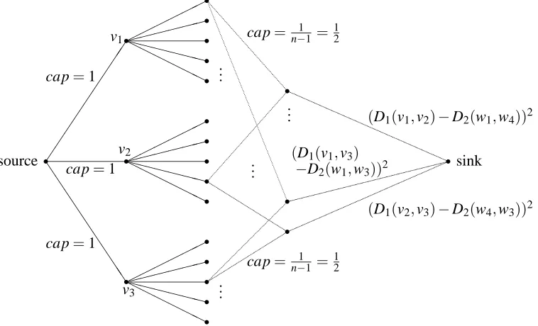
is incident with all n−1 other vertices and thus n−1 edges of the smaller graph are incident with each vertex. The complete construction is illustrated in Figure 11 for the problem from Figure 1.
r
source
cap=1
cap=1 J
J J
J J
J J
JJ cap=1
r
v1
r
v2
r
v3
XXXXXX
HH HH
HH
XXXXXX
HH HH
HH
XXXXXX
HH HH
HH
r
r
r
r
r
r
r
r
r
r
r
r
r
r
r
cap= n−11 =12
cap= 1 n−1=12 ..
.
.. .
.. .
r
r
r
..
. (D1(v1,v2)−D2(w1,w4))2 (D1(v1,v3)
−D2(w1,w3))2
(D1(v2,v3)−D2(w4,w3))2
rsink
Figure 11: Part of graph for an exact solution of the best approximation problem. The submodular flow constraints as well as arc orientations are not indicated. Arcs are directed in the general direction ”from left to right”. The arcs for which cost labels are specified refer to the solution for the problem from Figure 1.
A best graph approximation amounts to a cost minimal flow of strength n from source to sink such that the flows along the edges between all viand(vi,wj)are integer. The other constraints then imply that the flows are binary over these edges.
4.2 Branch and Bound
The complicated structure of the foregoing flow problem motivates to organize an exact best graph approximation by branch and bound. Subisomorphisms will be built up sequentially by either prun-ing or refinprun-ing a partial subisomorphism. A partial subisomorphism is a subisomorphism defined over a subset of the vertex set of the smaller graph. The domain of a partial subisomorphism is de-noted by A(V1)and the partial subisomorphism itself is denoted byϕ|A(V1). The special case of the
partial subisomorphism being defined over the complete vertex set of the smaller graph is denoted byϕ=ϕ|V1.
A lower bound for the approximation distance of a partial subisomorphism can be obtained by independently minimizing distances between unassigned and assigned vertices. Formally, the lower bound is given by
∑
{vi,vj}∈E1
≥
∑
{vi,vj}∈E1,vi,vj∈A(V1)
D1(vi,vj)−D2(ϕ(vi),ϕ(vj)) 2
+
∑
v0∈A(V1)c(v0)2 =: Val(ϕ|A(V1)),
where c(v0) =minv∈V1−A(V1),w∈V2−ϕ(A(V1))|D1(v0,v)−D2(ϕ(v0),w)|for all v0∈A(V1).
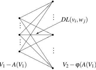
Improved lower bounds can be constructed by cost minimal assignments in analogy to the heuristic distance list constructions of Section 3. Independent minimization over unassigned ver-tices is replaced by joint minimization. The vertex set of the bipartite graph for the assignment
problem consist of both sets of unassigned vertices which are V1−A(V1)and V2−ϕ(A(V1)). The
cost values of the edges are given by squared errors of distance list approximations DL(v,w), see Figure 12.
r
.. .
r
.. .
r
V1−A(V1) r
.. .
r
.. .
r
V2−ϕ(A(V1))
HH HH
HH J
J J
J J
J J
JJ
DL(vi,wj)
@
@ @
@ @
@
HH HH
HH
Figure 12: Assignment problem for improved lower bound of partial subisomorphismϕ|A(V1).
The improved lower bound is
∑
{vi,vj}∈E1
D1(vi,vj)−D2(ϕ(vi),ϕ(vj)) 2
≥
∑
{vi,vj}∈E1,vi,vj∈A(V1)
D1(vi,vj)−D2(ϕ(vi),ϕ(vj)) 2
+val(ϕ|A(V1))
=: Val∗(ϕ|A(V1)),
where val(ϕ|A(V1)) is the minimum cost value of the lower bounding assignment problem from
Figure 12. The bounding strategy of a branch and bound algorithm for best graph approximation can now be readily specified as follows.
Bound
Case A(V1)6=V1.
If Val∗(ϕ|A(V1))≤M then refineϕ|A(V1) else ignoreϕ|A(V1). (pruneorbound).
Case A(V1) =V1.
If Val∗(ϕ) =M then Lopt=Lopt∪ {ϕ}.
If Val∗(ϕ)<M then Lopt={ϕ}and M=Val∗(ϕ).
The value M is the approximation distance of the best subisomorphism found so far and Lopt is
The algorithm operates on a list U of unexplored partial subisomorphisms until this list becomes empty. The initial setting of this list consists of partial subisomorphisms that make exactly one assignment.
B+B
1. Input graphs G1,G2with distances D1,D2.
Initialization. M cost of arbitrary subisomorphism. U={ϕ|v1(v1) =w1, . . . ,ϕ|v1(v1) =wm}.
Lopt=/0. 2. While U 6=/0do
(a) Selectionϕ|A(V1)∈U .
(b) U=U− {ϕ|A(V1)}.
(c) Computation of Val∗(ϕ|A(V1)).
(d) (Bound)
If A(V1) =V1then
If Val∗(ϕ) =M then Lopt=Lopt∪ {ϕ}.
If Val∗(ϕ)<M then Lopt={ϕ}and M=Val∗(ϕ). (e) (Branch)
If Val∗(ϕ|A(V1))<M then U=U∪S
w0∈V2−ϕ(A(V1)){ϕ|A(V1)∪{v0}with
ϕ|A(V1)∪{v0}(v0) =w0}for one v0∈A(V1).
3. Output list of optimal subisomorphisms Lopt.
The branch and bound procedure is informal in so far as the selection step 2(a) and the branching step 2(e) leave many ways of specialization. Removal is specified implicitly here which means that a partial subisomorphism selected in step 2(a) is removed anyway in step 2(b). Refinements of the partial subisomorphism are possibly added to U in the branching step. Whenever a partial subisomorphism is not pruned by the bounding step, the next iteration of step 2 may or may not select a refinement of this partial subisomorphism to continue with.
5. Conclusion
Best graph approximation has been formulated for labeled graphs in analogy to isomorphism for unlabeled graphs. Polynomial time approximation algorithms in terms of linear assignment prob-lems have been given and exact algorithms have been outlined. All algorithms are independent from application domains.
Whenever an instance graph is to be matched to several instead of one model graph, this can obviously be done sequentially. The best match is given by the minimum over all approximation distances and a ranking of the matching results is given by increasingly sorted approximation dis-tances.
References
Endika Bengoetxea. Inexact graph matching using estimation of distribution algorithms. Ph.D. dis-sertation, University of the Basque Country, San Sebastian, 2002.
Tiberio S. Caetano, Terry Caelli, Dale Schuurmanns and Dante A.C Barone. Graphical models and point pattern matching. IEEE Transactions on Pattern Analysis and Machine Intelligence PAMI, forthcoming.
Pierre-Antoine Champin and Christine Solnon. Measuring the similarity of labeled graphs. In Pro-ceedings of the Fifth International Conference on Case-Based Reasoning, pages 80-95, Springer, LNCS 2689, Berlin, 2003.
Richard Desper and Martin Vingron. Tree fitting: topological reconstruction from ordinary least-squares edge length estimates. Journal of Classification, 19:87-112, 2002.
Ian Foster and Carl Kesselman, editors. The Grid: Blueprint to a new Computing Infrastructure. 2nd ed., Elsevier, Amsterdam, 2004.
Satoru Fujishige. Submodular Functions and Optimization. North Holland, Amsterdam, 1991.
Michael R. Garey and David S. Johnson. Computers and Intractability. Freeman, San Francisco, 1981.
Steven Gold and Anand Rangarajan. A graduated assignment algorithm for graph matching. IEEE Transactions on Pattern Analysis and Machine Intelligence. 18:377-388, 1996.
Gene H. Golub and Charles F. van Loan. Matrix Computations. 4th printing, John Hopkins Univer-sity Press, Baltimore, 1985.
Godefrey H. Hardy, John E. Littlewood and George Polya. Inequalities. Cambridge University Press, Cambridge, 1948.
Adel Hlaoui and Shengrui Wang. A new algorithm for inexact graph matching. In Proceedings of the International Conference on Pattern Recognition ICPR’02, pages 180-183, Quebec, 2002.
Thomas K¨ampke. Scalable distance similarity of chemical structures. Combinatorial Chemistry and High Throughput Screening. 7:11-21, 2004.
Sergey Melnik, Hector Garcia-Molina and Erhard Rahm. Similarity flooding: a versatile graph matching algorithm and its application to schema matching. In Proceedings of the 16th Interna-tional Conference on Data Engineering ICDE, 12 pages, San Diego, 2002.
Kurt Mehlhorn and Stephan N¨aher. LEDA A Platform for Combinatorial and Geometric Computing. Cambridge University Press, Cambridge, 2000.
Bruno T. Messmer and Horst Bunke. A new algorithm for error-tolerant subgraph isomorphism detection. IEEE Transactions on Pattern Analysis and Machine Intelligence PAMI, 20:493-504, 1998.
Apostolos N. Papadopoulos and Yannis Manolopoulos. Structure-based similarity search with graph histograms. In Proceedings of the 10th International Workshop on Database and Expert System Applications DEXA, pages 174-178, 1999.
Arthur R. Pope and David G. Lowe. Learning appearance models for object recognition. In Proceed-ings of International Workshop on Object Representation for Computer Vision, pages 201-219, Springer, Berlin, 1996.
Dennis Shasha, Jason T.L. Wang and Rosalba Giugno. Algorithmics and applications of tree and graph searching. In Proceedings of the Symposium on Principles of Database Systems, pages 39-52, 2002.
Steven S. Skiena and Gopalakrishnan Sundaram. A partial digest approach to restriction site map-ping. Bulletin of Mathematical Biology, 56:275-294, 1994.
Jason T.L. Wang, Bruce A. Shapiro, Dennis Shasha, Kaizhong Zhang and Kathleen M. Currey. An algorithm for finding the largest approximately common substructures of two trees. IEEE Transactions on Pattern Analysis and Machine Intelligence, 20:889-895, 1998.
Laurenz Wiskott, Jean-Marc Fellous, Norbert Kr ¨uger, Christoph Malsburg. Face recognition by elastic bunch graph matching. IEEE Transactions on Pattern Analysis and Machine Intelligence PAMI, 19:775-779, 1997.