Maximum-Gain Working Set Selection for SVMs
Tobias Glasmachers [email protected]
Christian Igel [email protected]
Institut f¨ur Neuroinformatik Ruhr-Universit¨at Bochum 44780 Bochum, Germany
Editors: Kristin P. Bennett and Emilio Parrado-Hern´andez
Abstract
Support vector machines are trained by solving constrained quadratic optimization problems. This is usually done with an iterative decomposition algorithm operating on a small working set of vari-ables in every iteration. The training time strongly depends on the selection of these varivari-ables. We propose the maximum-gain working set selection algorithm for large scale quadratic programming. It is based on the idea to greedily maximize the progress in each single iteration. The algorithm takes second order information from cached kernel matrix entries into account. We prove the con-vergence to an optimal solution of a variant termed hybrid maximum-gain working set selection. This method is empirically compared to the prominent most violating pair selection and the lat-est algorithm using second order information. For large training sets our new selection scheme is significantly faster.
Keywords: working set selection, sequential minimal optimization, quadratic programming,
sup-port vector machines, large scale optimization
1. Introduction
We consider 1-norm support vector machines (SVM) for classification. These classifiers are usually trained by solving convex quadratic problems with linear constraints. For large data sets, this is typ-ically done with an iterative decomposition algorithm operating on a small working set of variables in every iteration. The selection of these variables is crucial for the training time.
Recently, a very efficient SMO-like (sequential minimal optimization using working sets of size 2, see Platt, 1999) decomposition algorithm was presented by Fan et al. (2005). The main idea is to consider second order information to improve the working set selection. Independent from this approach, we have developed a working set selection strategy sharing this basic idea but with a different focus, namely to minimize the number of kernel evaluations per iteration. This considerably reduces the training time of SVMs in case of large training data sets. In the following, we present our approach, analyze its convergence properties, and present experiments evaluating the performance of our algorithm. We close with a summarizing conclusion.
1.1 Support Vector Machine Learning
corre-sponding class labels yi=±1. A positive semi-definite kernel function k :
X
×X
→Rensures theexistence of a feature Hilbert space
F
with inner producth·,·iand a mappingΦ:X
→F
such thatk(xi,xj) =hΦ(xi),Φ(xj)i.
The SVM algorithm constructs a real-valued, affine linear function H on the feature space. The corresponding function h :=H◦Φon the input space can be computed in terms of the kernel k with-out the need for explicit computations in
F
. The zero set of H is called the separating hyperplane, because the SVM uses the sign of this function for class prediction. This affine linear function is defined through maximizing the margin, that is, the desired distance of correctly classified training patterns from the hyperplane, and reducing the sum of distances by which training examples violate this margin. The trade-off between these two objectives is controlled by a regularization parameterC>0.
Training a 1-norm soft margin SVM is equivalent to solving the followingℓ-dimensional convex quadratic problem with linear constraints forα∈Rℓ:
P
maximize f(α) =vTα−12αTQα
subject to yTα=z
and 0≤αi≤C , ∀i∈ {1, . . . , ℓ} .
The requirements yTα=z and 0≤α
i≤C are referred to as equality constraint and box constraints, respectively. In the SVM context the constants v∈Rℓand z∈Rare fixed to v= (1, . . . ,1)T and z=0. The matrix Q∈Rℓ×ℓ is defined as Qi j:=yiyjk(xi,xj) and is positive semi-definite as the
considered kernel function k is positive semi-definite. The vector y := (y1, . . . ,yℓ)T, yi∈ {+1,−1} for 1≤i≤ℓ, is composed of the labels of the training patterns x1, . . . ,xℓ. The set of points α fulfilling the constraints is called the feasible region
R
(P)of problemP
.An optimal solutionα∗of this problem defines the function h(x) =∑ℓi=1α∗iyik(xi,x) +b, where the scalar b can be derived fromα∗ (e.g., see Cristianini and Shawe-Taylor, 2000; Sch¨olkopf and Smola, 2002).
1.2 Decomposition Algorithms
Making SVM classification applicable in case of large training data sets requires an algorithm for the solution of
P
that does not presuppose theℓ(ℓ+1)/2 independent entries of the symmetric matrix Q to fit into working memory. The methods of choice in this situation are the so called decomposition algorithms (Osuna et al., 1997). These iterative algorithms start at an arbitrary feasible pointα(0) and improve this solution in every iteration t fromα(t−1) toα(t)until some stopping condition is satisfied. In each iteration an active set or working set B(t) ⊂ {1, . . . , ℓ} is chosen. Its inactive complement is denoted by N(t):={1, . . . , ℓ} \B(t). The improved solution α(t) may differ from α(t−1)only in the components in the working set, that is,α(t−1)i =α (t)
Decomposition Algorithm
α(0)←feasible starting point, t←1 1
repeat
2
select working set B(t) 3
solve QP restricted to B(t)resulting inα(t) 4
t←t+1 5
until stopping criterion is met
6
The sub-problem defined by the working set in step 4 has the same structure as the full problem
P
but with only q variables.1 Thus, the complete problem description fits into the available working memory and is small enough to be solved by standard tools.For the SVM problem
P
the working set must have a size of at least two. Indeed, the sequen-tial minimal optimization (SMO) algorithm selecting working sets of size q=2 is a very efficient method (Platt, 1999). The great advantage of the SMO algorithm is the possibility to solve the sub-problem analytically (cf. Platt, 1999; Cristianini and Shawe-Taylor, 2000; Sch¨olkopf and Smola, 2002).1.3 Working Set Selection
Step 3 is crucial as the convergence of the decomposition algorithm depends strongly on the work-ing set selection procedure. As the selection of the workwork-ing set of a given size q that gives the largest improvement in a single iteration requires the knowledge of the full matrix Q, well working heuristics for choosing the variables using less information are needed.
There exist various algorithms for this task, an overview is given in the book by Sch¨olkopf and Smola (2002). The most prominent ones share the strategy to select pairs of variables that mostly violate the Karush-Kuhn-Tucker (KKT) conditions for optimality and can be subsumed under the
most violating pair (MVP) approach. Popular SVM packages such as SVMlightby Joachims (1999) and LIBSVM 2.71 by Chang and Lin (2001) implement this technique. The idea of MVP is to select one or more pairs of variables that allow for a feasible step and most strongly violate the KKT conditions.
Here we describe the approach implemented in the LIBSVM 2.71 package. Following Keerthi and Gilbert (2002) we define the sets
I :={i∈ {1, . . . , ℓ}|yi= +1∧α(it−1)<C} ∪ {i∈ {1, . . . , ℓ}|yi=−1∧α(it−1)>0}
J :={i∈ {1, . . . , ℓ}|yi= +1∧α(it−1)>0} ∪ {i∈ {1, . . . , ℓ}|yi=−1∧α(it−1)<C} . Now the MVP algorithm selects the working set B(t)={b1,b2}using the rule
b1:=argmax i∈I
yi ∂f
∂αi (α)
b2:=argmin i∈J
yi ∂f
∂αi (α)
.
The condition yb1 ∂f
∂αb1(α)−yb2 ∂f
∂αb2(α)<ε is used as the stopping criterion. In the limit ε→0
the algorithm checks the exact KKT conditions and only stops if the solution found is optimal. The MVP algorithm is known to converge to the optimum (Lin, 2001; Keerthi and Gilbert, 2002; Takahashi and Nishi, 2005).
SVMlightuses essentially the same working set selection method with the important difference that it is not restricted to working sets of size 2. The default algorithm selects 10 variables by picking the five most violating pairs. In each iteration an inner optimization loop determines the solution on the 10-dimensional sub-problem up to some accuracy.
Fan et al. (2005) propose a working set selection procedure which uses second order informa-tion. The first variable b1 is selected as in the MVP algorithm. The second variable is chosen in a way that promises the maximal value of the target function f ignoring the box constraints. The selection rule is
b2:=argmax i∈J
f(αmax {b1,i})
.
Here,αmax{b
1,i}is the solution of the two-dimensional sub-problem defined by the working set{b1,i}
at positionα(t−1)considering only the equality constraint. For this second order algorithm costly kernel function evaluations may become necessary which can slow down the entire algorithm. These kernel values are cached and can be reused in the gradient update step, see equation (2) in Section 2.1. Because this algorithm is implemented in version 2.8 of LIBSVM, we will refer to it as the LIBSVM-2.8 algorithm.
The simplest feasible point one can construct is α(0)= (0, . . . ,0)T, which has the additional advantage that the gradient∇f(α(0)) =v= (1, . . . ,1)Tcan be computed without kernel evaluations. It is interesting to note that in the first iteration starting from this point all components of the gradient ∇f(α(0))of the objective function are equal. Thus, the selection schemes presented above have a freedom of choice for the selection of the first working set. In case of LIBSVM, for b1simply the variable with maximum index is chosen in the beginning. Therefore, the order in which the training examples are presented is important in the first iteration and can indeed significantly influence the number of iterations and the training time in practice.
Other algorithms select a rate certifying pair (Hush and Scovel, 2003). The allurement of this approach results from the fact that analytical results have been derived not only about the guaranteed convergence of the algorithm, but even about the rate of convergence (Hush and Scovel, 2003; List and Simon, 2005). Unfortunately, in practice these algorithms seem to perform rather poorly.
1.4 Related Methods
The SimpleSVM algorithm developed by Vishwanathan et al. (2003) provides an alternative to the decomposition technique. It can handle a wide variety of SVM formulations, but is limited in the large scale context by its extensive memory requirements. In contrast, Keerthi et al. (2000) present a geometrically inspired algorithm with modest memory requirements for the exact solution of the SVM problem. A drawback of this approach is that it is not applicable to the standard one-norm slack penalty soft margin SVM formulation, which we consider here, because it requires the classes to be linearly separable in the feature space
F
.2. Maximum-Gain Working Set Selection
Before we describe our new working set selection method, we recall how the quadratic problem re-stricted to a working set can be solved (cf. Platt, 1999; Cristianini and Shawe-Taylor, 2000; Chang and Lin, 2001). Then we compute the progress, the functional gain, that is achieved by solving a single sub-problem. Picking the variable pair maximizing the functional gain while minimizing ker-nel evaluations—by reducing cache misses when looking up rows of Q—leads to the new working set selection strategy.
2.1 Solving the Problem Restricted to the Working Set
In every iteration of the decomposition algorithm all variables indexed by the inactive set N are fixed and the problem
P
is restricted to the variables indexed by the working set B={b1, . . . ,bq}. We defineαB= (αb1, . . . ,αbq)
T , Q
B=
Qb1b1 . . . Qbqb1
..
. . .. ...
Qb1bq . . . Qbqbq
, yB= (yb1, . . . ,ybq)
T
and fix the values
vB= 1−
∑
i∈N
Qib1αi, . . . ,1−
∑
i∈N
Qibqαi
!T
∈Rq and zB=−
∑
i∈N
yiαi∈R
not depending onαB. This results in the convex quadratic problem (see Joachims, 1999)
P
B,α
maximize fB(αB) =vTBαB−12αTBQBαB subject to yTBαB=zB
and 0≤αi≤C ∀i∈B .
The value zB can easily be determined in time linear in q, but the computation of vB takes time linear in q andℓ. Then
P
B,α can be solved using a ready-made quadratic program solver in time independent ofℓ.We will deal with this problem under the assumption that we know the gradient vector
G :=∇fB(αB) =
∂
∂αb1
fB(αB), . . . , ∂ ∂αbq
fB(αB)
T
(1)
of partial derivatives of fB with respect to all q variablesαb1, . . . ,αbq indexed by the working set.
∇f(αB)
∇f(α∗B)
αB
α∗ B
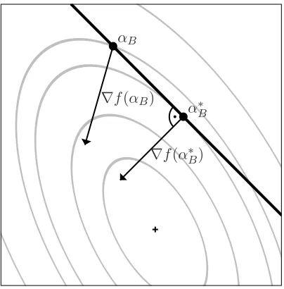
Figure 1: The 2-dimensional SMO sub-problem restricted to the equality constraint (solid ‘feasible’ line) and the box constraints (boundary). The point fulfilling the equality constraint with gradient orthogonal to the feasible line is a candidate for the solution of the sub-problem. If it is not feasible w.r.t. the box constraints it has to be moved along the line onto the box boundary.
the equality constraint restricts us to a line. Due to the box constraints only a bounded segment of this line is feasible (see Figure 1). To solve the restricted problem we define the vector wB := (1,−yb1yb2)
T pointing along the 1-dimensional feasible hyperplane. To find the maximum on this
line we look at the gradient∇fB(αB) =vB−QBαBand compute the step µB·wB(µB∈R) such that the gradient∇fB(αB+µB·wB)is orthogonal to wB,
0=h∇fB(αB+µBwB),wBi =hvB−QBαB−µBQBwB,wBi =h∇fB(αB)−µBQBwB,wBi .
Using∇fB(αB) = (Gb1,Gb2)
T we get the solution
µmaxB = (Gb1−yb1yb2Gb2)/(Qb1b1+Qb2b2−2yb1yb2Qb1b2) .
The corresponding point on the feasible line is denoted byαmaxB =αB+µmaxB wB. Of course,αmaxB is not necessarily feasible. We can easily apply the box constraints to µmaxB . The new solution clipped to the feasible line segment is denoted µ∗B. The maximum of
P
B,αcan now simply be expressed as α∗B=αB+µ∗BwB.
After the solution of the restricted problem the new gradient
has to be computed. As the formula indicates this is done by an update of the former gradient. Because∆α=α(t)−α(t−1) differs from zero in only the b1th and b2th component only the corre-sponding two matrix rows of Q have to be known to determine the update.
2.2 Computing the Functional Gain
Expressing the target function on the feasible line by its Taylor expansion in the maximumαmaxB we get
˜
fB(ξ):=fB(αmaxB +ξwB) =fB(αmaxB )−
1 2(ξwB)
TQ B(ξwB)
=fB(αmaxB )−
1 2w
T BQBwB
ξ2 .
Now it is possible to calculate the gain as
fB(α∗B)−fB(αB) = f˜B(µ∗B−µmaxB )−f˜B(0−µmaxB ) =
1 2w
T BQBwB
((µmaxB )2−(µ∗
B−µmaxB )2) =
1 2w
T BQBwB
(µ∗B(2µmaxB −µ∗B)) =1
2(Qb1b1+Qb2b2−2yb1yb2Qb1b2)(µ∗B(2µ
max
B −µ∗B)) . (3)
The diagonal matrix entries Qiineeded for the calculation can be precomputed before the decom-position loop starts using time and memory linear inℓ. Thus, knowing only the derivatives (1), C,
yB, and Qb1b2 (and the precomputed diagonal entries) makes it possible to compute the gain in f .
Usually in an SVM implementation the derivatives are already at hand because they are required for the optimality test in the stopping criterion. Of course we have access to the labels and the regu-larization parameter C. The only remaining quantity needed is Qb1b2, which unfortunately requires
evaluating the kernel function.
2.3 Maximum-Gain Working Set Selection
Now, a straightforward working set selection strategy is to look at allℓ(ℓ−1)/2 possible variable pairs, to evaluate the gain (3) for every one of them, and to select the best, that is, the one with maximum gain. It can be expected that this greedy selection policy leads to very fast convergence measured in number of iterations needed. However, it has two major drawbacks making it advisable only for very small problems: looking at all possible pairs requires the knowledge of the complete matrix Q. As Q is in general too big to fit into the working memory, expensive kernel function evaluations become necessary. Further, the evaluation of all possible pairs scales quadratically with the number of training examples.
the gradient update (2). This fact leads to the following maximum-gain working pair selection (MG) algorithm:
Maximum-Gain Working Set Selection in step t
if t=1 then 1
select arbitrary working set B(1)={b1,b2},yb1 6=yb2
2
else
3
select pair B(t)← argmax
B={b1,b2}|b1∈B(t−1),b2∈{1,...,ℓ} gB(α) 4
In the first iteration, usually no cached matrix rows are available. Thus, an arbitrary working set
B(1)={b1,b2}fulfilling yb1 6=yb2 is chosen. In all following iterations, given the previous working
set B(t−1)={b1,b2}, the gain of all combinations{b1,b}and{b2,b}(b∈ {1, . . . , ℓ}) is evaluated and the best one is selected.
The complexity of the working set selection is linear in the number of training examples. It is important to note that the algorithm uses second order information from the matrix cache. These information are ignored by all existing working set selection strategies, albeit they are available for free, that is, without spending any additional computational effort. This situation is comparable to the improvement of using the gradient for the analytical solution of the sub-problem in the SMO algorithm. Although the algorithm by Fan et al. (2005) considers second order information, these are in general not available from the matrix cache.
The maximum gain working pair selection can immediately be generalized to the class of
maximum-gain working set selection algorithms (see Section 2.5). Under this term we want to
subsume all working set selection strategies choosing variables according to a greedy policy with respect to the functional gain computed using cached matrix rows. In the following, we restrict ourselves to the selection of pairs of variables as working sets.
In some SVM implementations, such as LIBSVM, the computation of the stopping condition is done using information provided during the working set selection. LIBSVM’s MVP algorithm stops if the sum of the violations of the pair is less than a predefined constantε. The simplest way to implement a roughly comparable stopping condition in MG is to stop if the value µ∗Bdefining the length of the constrained step is smaller thanε.
It is worth noting that the MG algorithm does not depend on the caching strategy. The only requirement for the algorithm to efficiently profit from the kernel cache is that the cache always contains the two rows of the matrix Q that correspond to the previous working set. This should be fulfilled by every efficient caching algorithm, because recently active variables have a high proba-bility to be in the working set again in future iterations. That is, the MG algorithm does not require a change of the caching strategy. Instead, it improves the suitability of all caching strategies that at least store the information most recently used.
2.4 Hybrid Maximum-Gain Working Set Selection
Hybrid Maximum-Gain Working Set Selection in step t, 0<η≪1
if t=1 then 1
select arbitrary working set B(1)={b1,b2},yb1 6=yb2
2
else
3
if∀i∈B(t−1):α
i≤η·C∨αi≥(1−η)·C then 4
select B(t)according to MVP 5
else
6
select pair B(t)← argmax
B={b1,b2}|b1∈B(t−1),b2∈{1,...,ℓ} gB(α) 7
In the first iteration, usually no cached matrix rows are available. Thus, an arbitrary working set {b1,b2}fulfilling yb1 6=yb2 is selected. If in iteration t>1 both variables indexed by the previous
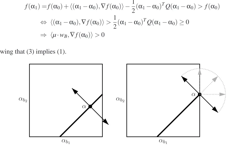
working set B(t−1)={b1,b2}are no more thanη·C, 0<η≪1, from the bounds, then the MVP algorithm is used. Otherwise the working set is selected according to MG. Figure 2 illustrates the HMG decision rule. The stopping condition tested by the decomposition algorithm is the one
∇
0
Cη C(1−η)
C
0 Cη C(1−η) C αb1
αb2
Figure 2: Illustration of the HMG algorithm. The plain defined by the previous working set B(t−1)= {b1,b2} is drawn. If the algorithm ended up in one of the gray corners then the MVP algorithm is used in iteration t.
from the working set selection algorithm used in the current iteration. That is, the decomposition algorithm stops if yb1
∂f
∂αb1(α)−yb2 ∂f
∂αb2(α)or µ∗Bfalls below the thresholdεdepending on whether MVP or MG has been selected.
The HMG algorithm is a combination of MG and MVP using MVP only in special situations. In our experiments, we setη=10−8. This choice is arbitrary and makes no difference toη=0 in nearly all cases. In practice, in almost all iterations MG will be active. Thus, this algorithm inherits the speed of the MG algorithm. It is important to note thatη is not a parameter influencing the convergence speed (as long as the parameter is small) and is therefore not subject to tuning.
Theorem 1 We consider problem
P
. Let (α(t))t∈N be a sequence of feasible points produced by
the decomposition algorithm using the HMG policy. Then, the limit point of every convergent sub-sequence is optimal for
P
.The proof can be found in Section 3.
2.5 Generalization of the Algorithm
In the following, we discuss some of the potential variants of the basic MG or HMG algorithm. It is possible to use a larger set of precomputed rows, say, 10, for the working set selection. In the extreme case we can run through all cached rows of Q. Then the working set selection algorithm becomes quite time consuming in comparison to the gradient update. As the number of iterations does not decrease accordingly, as we observed in real world applications, we recommend to use only the two rows of the matrix from the previous working set. We refer to Section 4.6 for a comparison. A small change speeding up the working set selection is fixing one element of the working set in every iteration. When alternating the fixed position, every element is used two times successively. Only ℓ−2 pairs have to be evaluated in every iteration. Though leading to more iterations this policy can speed up the MG algorithm for small problems (see Section 4.6).
The algorithm can be extended to compute the gain for tuples of size q>2. It is a severe disadvantage that such sub-problems can not be solved analytically and an iterative solver has to be used for the solution of the sub-problem. Note that this becomes necessary also for every gain computation during the working set selection. To keep the complexity of the working set selection linear in ℓonly one element new to the working set can be evaluated. Due to this limitation this method becomes even more cache friendly. The enlarged working set size may decrease the number of iterations required, but at the cost of the usage of an iterative solver. This should increase the speed of the SVM algorithm only on large problems with extremely complicated kernels, where the kernel matrix does not fit into the cache and the kernel evaluations in every iteration take much longer than the working set selection.
3. Convergence of the Algorithms
In this section we discuss the convergence properties of the decomposition algorithm using MG and HMG working set selection. First, we give basic definitions and prove a geometrical criterion for optimality. Then, as a motivation and a merely theoretical result, we show some properties of the gain function and prove that the greedy strategy w.r.t. the gain converges to an optimum. Returning to our algorithm, we give a counter example proving that there exist scenarios where pure MG looking at pairs of variables may stop after finitely many iterations without reaching an optimum. Finally, we prove that HMG converges to an optimum.
3.1 Prerequisites
In our convergence analysis, we consider the limitε→0, that is, the algorithms only stop if the quantities checked in the stopping conditions vanish. We will discuss the convergence of the infinite sequence(α(t))
t∈Nproduced by the decomposition algorithm. If the decomposition algorithm stops
in some iteration t0atα(t0−1), then by convention we setα(t)←α(t0−1)for all t≥t0. The definition
close to the optimum considered in other proofs (Keerthi and Gilbert, 2002; Takahashi and Nishi, 2005).
The Bolzano-Weierstraß property states that every sequence on a compact set contains a con-vergent sub-sequence. Because of the compactness of
R
(P) the sequence (α(t))t∈N always
con-tains a convergent sub-sequence denoted (α(t))
t∈S with limit point α(∞). From the construction of the decomposition algorithm it follows that the sequence(f(α(t)))
t∈N increases monotonically.
The compactness of
R
(P)implies that it is bounded. It therefore converges and its limit f(α(∞)) does not depend on the choice of the convergent sub-sequence. The gain sequence gB(t)(α(t−1)) = f(α(t))−f(α(t−1))is non-negative and converges to zero. It will be the aim of this section to prove thatα(∞)is the maximizer of f within the feasible regionR
(P
)if the decomposition algorithm is used with HMG working set selection.List and Simon (2004) introduced the (technical) restriction that all principal 2×2 minors of Q have to be positive definite. For Theorem 4, which was shown by List and Simon (2004), and the proof of Lemma 9 (and thus of Theorem 1) we adopt this requirement. The assumption is not very restrictive because it does not require the whole matrix Q to be positive definite. If in contrast Q is indeed positive definite (for example for Gaussian kernels with distinct examples) then this property is inherited by the principal minors.2
If we fix any subset of variables of
P
at any feasible pointα∈R
(P)then the resulting restricted problem is again of the formP
. By analytically solving the problem restricted to a working set B we can compute the gain gB(α). The set VP :={α∈Rℓ|hy,αi=z}is the hyperplane defined bythe equality constraint. It contains the compact convex feasible region
R
(P). The set of possible working sets is denoted byB
(P):=BB⊂ {1, . . . , ℓ},|B|=2 . We call two working sets B1,B2∈
B
(P)related if B1∩B26=/0. With a working set B={b1,b2}, b1<b2, we associate the vector wB with components(wB)b1 =1,(wB)b2 =−yb1yb2and(wB)i=0 otherwise. It points into the directionin whichαcan be modified using the working set.
If a feasible pointαis not optimal then there exists a working set B on which it can be improved. This simply follows from the fact that there are working set selection policies based on which the decomposition algorithm is known to converge (Lin, 2001; Keerthi and Gilbert, 2002; Fan et al., 2005; Takahashi and Nishi, 2005). In this case the gain gB(α)is positive.
Next, we give a simple geometrically inspired criterion for the optimality of a solution.
Lemma 2 We consider the problem
P
. For a feasible pointα0the following conditions areequiv-alent:
1. α0is optimal.
2. h(α−α0),∇f(α0)i ≤0 for allα∈
R
(P).3. hµ·wB,∇f(α0)i ≤0 for all µ∈R, B∈
B
(P)fulfillingα0+µ·wB∈R
(P).Proof The proof is organized as(1)⇒(2)⇒(3)⇒(1). We consider the Taylor expansion
f(α) = f(α0) +h(α−α0),∇f(α0)i − 1
2(α−α0)
TQ(α−α 0)
of f in α0. Let us assume that (2) does not hold, that is, there exists α∈
R
(P) such that q := h(α−α0),∇f(α0)i>0. From the convexity ofR
(P)it follows thatαµ:=µα+ (1−µ)α0∈R
(P) for µ∈[0,1]. We further set r :=12(α−α0)
TQ(α−α
0)≥0 and haveh(αµ−α0),∇f(α0)i=µq and 1
2(αµ−α0)TQ(αµ−α0) =µ2r. We can chose µ0∈(0,1]fulfilling µ0q>µ20r. Then it follows
f(αµ0) = f(α0) +h(αµ0−α0),∇f(α0)i −
1
2(αµ0−α0)
TQ(α
µ0−α0) = f(α0) +µ0q−µ20r
> f(α0) ,
which proves thatα0is not optimal. Thus(1)implies(2). Of course (3) follows from (2). Now we assumeα0is not optimal. From the fact that there are working set selection policies for which the decomposition algorithm converges to an optimum it follows that there exists a working set B on whichα0 can be improved, which means gB(α0)>0. Letα1denote the optimum on the feasible line segment within
R
(P
)written in the formα1=α0+µ·wB. Using the Taylor expansion above atα1and the positive semi-definiteness of Q we getf(α1) =f(α0) +h(α1−α0),∇f(α0)i − 1
2(α1−α0) TQ(α
1−α0)> f(α0) ⇔ h(α1−α0),∇f(α0)i>
1
2(α1−α0) TQ(α
1−α0)≥0 ⇒ hµ·wB,∇f(α0)i>0
showing that (3) implies (1).
α
α
αb1
αb1
αb2
αb2
Figure 3: This figure illustrates the optimality condition given in Lemma 2 for one working set. On the left the case of two free variablesαb1andαb2 is shown, while on the right the variable
αb1 is at the bound C. The fat lines represent the feasible region for the 2-dimensional
3.2 Convergence of the Greedy Policy
Before we look at the convergence of the MG algorithm, we use Theorem 4 by List and Simon (2004) to prove the convergence of the decomposition algorithm using the greedy policy with respect to the gain for the working set selection. For this purpose we will need the concept of a 2-sparse witness of suboptimality.
Definition 3 (2-sparse witness of suboptimality) A family of functions(CB)B∈B(P)
CB:
R
(P)→R≥0fulfilling the conditions
(C1) CBis continuous,
(C2) ifαis optimal for
P
B,α, then CB(α) =0, and(C3) if a feasible pointαis not optimal for
P
, then there exists B such that CB(α)>0is called a 2-sparse witness of suboptimality (List and Simon, 2004).
Every 2-sparse witness of suboptimality induces a working set selection algorithm by
B(t):=argmax B∈B(P)
CB(α(t−1))
.
List and Simon (2004) call this the induced decomposition algorithm. Now we can quote a general convergence theorem for decomposition methods induced by a 2-sparse witness of suboptimality:3
Theorem 4 (List and Simon, 2004) We consider the problem
P
and a 2-sparse witness of subop-timality(CB)B∈B(P). Let(α(t))t∈Ndenote a sequence of feasible points generated by thedecompo-sition method induced by(CB)and(α(t))t∈Sa convergent sub-sequence with limit pointα(∞). Then,
the limit point is optimal for
P
.The following lemma allows for the application of this theorem.
Lemma 5 The family of functions(gB)B∈B(P)is a 2-sparse witness of suboptimality.
Proof Property (C2) is fulfilled directly per construction. Property (C3) follows from the fact
that there exist working set selection strategies such that the decomposition method converges (Lin, 2001; Takahashi and Nishi, 2005; List and Simon, 2005). It is left to prove property (C1). We fix a working set B={b1,b2}and the corresponding direction vector wB. Choosing the working set B is equivalent to restricting the problem to this direction. We define the affine linear function
ϕ: VP →R , α7→
∂ ∂µ
µ=0
f(α+µwB)
and the ((ℓ−2)-dimensional) hyperplane H :={α∈VP|ϕ(α) =0}within the ((ℓ−1)-dimensional)
vector space VP. This set always forms a hyperplane because QwB6=0 is guaranteed by the as-sumption that all 2×2 minors or Q are positive definite. This hyperplane contains the optima of f restricted to the linesα+R·wBconsidering the equality constraint but not the box constraints. We
introduce the mapπH projecting VP onto H along wB, that is the projection mapping the whole line
α+R·wB onto its unique intersection with H. The hyperplane H contains the compact subset
˜
H :=
α∈Hα+R·wB∩
R
(P)6=/0 =πH(R(P))on which we define the function
δ: ˜H→R , α7→ argmin
{µ∈R|α+µwB∈R(P)}|
µ| .
The termδ(πH(α))wB describes the shortest vector movingα∈H to the feasible region on the line˜ along wB. On ˜H\
R
(P)it parameterizes the boundary of the feasible region (see Figure 4). These properties enable us to describe the optimal solution of the sub-problem induced by the working set. Starting fromα∈R
(P)the optimumπH(α)is found neglecting the box constraints. In case this point is not feasible it is clipped to the feasible region by moving it byδ(πH(α))wB. Thus, per construction it holds gB(α) =f(πH(α) +δ(πH(α))wB)−f(α). The important point here is that convexity and compactness ofR
(P)guarantee thatδis well-defined and continuous. We conclude that gBis continuous as it is a concatenation of continuous functions.R(P)
H
˜
H wB
Figure 4: The feasible region
R
(P)within the(ℓ−1)-dimensional vector space VP is illustrated.Theℓ-dimensional box constraints are indicated in light gray. The thin line represents the hyperplane H containing the compact subset ˜H drawn as a fat line segment. The lengths
of the dotted lines indicate the absolute values of the functionδ on ˜H. The function δ
vanishes within the intersection of ˜H and
R
(P).Corollary 6 We consider problem
P
. Let(α(t))t∈N be a sequence of feasible points produced by
the decomposition algorithm using the greedy working set selection policy. Then, every limit point
α(∞)of a converging sub-sequence(α(t))
t∈Sis optimal for
P
.Proof For a feasible pointαand a working set B the achievable gain is computed as gB(α). Thus, the decomposition method induced by the family(gB)selects the working set resulting in the maximum gain, which is exactly the greedy policy. Lemma 5 and Theorem 4 complete the proof.
3.3 Convergence of the MG Algorithm
Theorem 7 Given a feasible pointα(t)for
P
and a previous working set B(t−1)of size 2 as a starting point. Then, in general, the MG algorithm may get stuck, that means, it may stop after finitely many iterations without reaching an optimum.Proof As a proof we give a counter example. The MG algorithm may get stuck before reaching the
optimum because it is restricted to reselect one element of the previous working set. Forℓ <4 this poses no restriction. Thus, to find a counter example, we have to use someℓ≥4. Indeed, using four training examples is already sufficient. We consider
P
forℓ=4 with the valuesQ=
2 √3 1 √3
√
3 4 √3 3
1 √3 2 √3
√
3 3 √3 4
, C= 1
10 , y=
−1 −1 +1 +1 .
The matrix Q is positive definite with eigenvalues(9,1,1,1). We assume the previous working set to be B(1)={1,3}resulting in the pointα(1)= (C,0,C,0)T. Note that this is the result of the first iteration starting fromα(0)= (0,0,0,0)greedily choosing the working set B(1)={1,3}. It is thus possible that the decomposition algorithm reaches this state in the SVM context. We compute the gradient
∇f(α(1)) =1−Qα(1)= ( 7 10,1−
√ 3 5 ,
7 10,1−
√ 3 5 )
T≈(0.7,0.65,0.7,0.65)T
(which is orthogonal to y). Using Lemma 2 we compute that the sub-problems defined by all work-ing sets with exception B={2,4}are already optimal. The working sets B(1)and B have no element in common. Thus, the maximum gain working pair algorithm cannot select B(2)=B and gets stuck
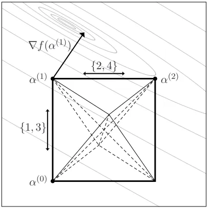
although the pointα(1)is not optimal. From Figure 5 we can see that the same example works for all points on the edgeα(1)= (C,ν,C,ν)forν∈[0,C). Lemma 8 states that indeed the edges of the octahedron are the only candidates for the MG algorithm to get stuck.
3.4 Convergence of the HMG Algorithm
The above result makes it advisable to use a different algorithm whenever MG is endangered to get stuck. For this purpose the HMG algorithm was designed. In this section we prove that this modification indeed guarantees convergence to an optimum.
The following lemma deals with the specific property of the MG algorithm to reselect one element of the working set, that is, to select related working sets in consecutive iterations. It is a major building block in the proof of the main result stated in Theorem 1.
Lemma 8 We consider
P
, a current non-optimal feasible pointαand a previous working set B1= {b1,b2}. If at least one of the variablesαb1 andαb2 is free (not at the bounds 0 or C) then there exists a working set B2related to B1such that positive gain gB2(α)>0 can be achieved.Proof We show that no counter example exists. The idea is to reduce the number of possible
α(0)
α(1) α(2)
∇f(α(1))
{1,3}
{2,4}
Figure 5: Illustration of the counter example. The feasible region
R
(P)forms an octahedron within the 3-dimensional space VP. The possible directions of movement using working sets ofsize 2 are parallel to the edges of the octahedron. The SVM algorithm starts inα(0)= (0,0,0,0)T. During the first two iterations the greedy policy reaches the points α(1)= (C,0,C,0)Tandα(2)= (C,C,C,C)T. The MG algorithm gets stuck after the first iteration atα(1). The plane spanned by the directions(1,0,1,0)T and(0,1,0,1)T defined by the working sets{1,3}and{2,4}respectively, is drawn. The gray lines are level sets of the target function f within this plane. In the pointα(1) the gradient∇f(α(1))(which lies within the plane) has an angle of less thanπ/2 only with the horizontally drawn edge corresponding to the working set{2,4}.
Forℓ≤3 the condition that B1and B2are related is no restriction and we are done. In the main part of the proof, we consider the 4-dimensional case and setα= (α1,α2,α3,α4)T and B1={1,2} with free variableα1∈(0,C). In the end, we will reduce the general case toℓ≤4.
Let us have a look at potential counter examples. A feasible pointαis a counter example if it is not optimal and does not allow for positive gain on any working set related to B1. These conditions are equivalent to
gB(α)
(
=0 for B6={3,4}
>0 for B={3,4} . (4)
Looking at the six possible working sets B we observe from Lemma 2 that we have to distinguish three cases for sub-problems induced by the working sets:
• The current point α is at the bounds for a variable indexed by B and the points α+µ·
wB lie within
R
(P) only for µ≤0. Then Lemma 2 states that α can only be optimal if• The current point α is at the bounds for a variable indexed by B and the points α+µ·
wB lie within
R
(P) only for µ≥0. Then Lemma 2 states that α can only be optimal ifhwB,∇f(α)i ≤0.
• The current point α is not at the bounds for both variables indexed by B. Thus, there are positive and negative values for µ such thatα+µ·wB lies within
R
(P). From Lemma 2 it follows thatαcan only be optimal ifhwB,∇f(α)i=0.We conclude that the signs (<0,=0, or>0) of the expressions
hwB,∇f(α)i= ∂f
∂αb′0
(α)−yb′
0yb′1
∂f
∂αb′1
(α) for B={b0′,b′1} ⊂ {1,2,3,4} (5) and the knowledge about which variables are at which bound are sufficient for the optimality check. Further, it is not important which exact value a free variable takes. The possible combinations of vectors wBoccurring in equation (5) are generated by the label vector y. Combining these insights, we define the maps
sign :R→ {−1,0,+1}, x7→
−1 if x<0
0 if x=0
+1 if x>0
bound :[0,C]→ {0,C
2,C}, x7→
0 if x=0
C
2 if 0<x<C
C if x=C
and a mapping of all possible counter examples onto a finite number of cases
Ψ:
R
(P)×R4× {−1,+1}4→ {−1,0,+1}6× {0,C/2,C}3× {−1,+1}4,
α ∇f(α)
y
7→
bound(αi),i∈ {2,3,4} sign(hwB,∇f(α)i),B∈
B
(P)y
.
A possible counter example is fully determined by a candidate pointα∈
R
(P), the gradient G=∇f(α), and the label vector y. As the parameters of problem
P
are not fixed here, the equality constraint can be ignored, because every point fulfilling the box constraints can be made feasible by shifting the equality constraint hyperplane. The relation Ψ(α,G,y) =Ψ(α˜,G˜,y˜) divides the pre-image ofΨinto equivalence classes. For each element of one equivalence class the check of condition (4) using Lemma 2 is the same. Formally, we haveΨ(α,G,y) =Ψ(α˜,G˜,y˜)
⇒condition (4) holds for(α,G,y)if and only if condition (4) holds for(α˜,G˜,y˜) .
It follows that any finite set containing representatives of all the non-empty equivalence classes is sufficient to check for the existence of a counter example in the infinite pre-image ofΨ.4 The checking can be automated using a computer program. A suitable program can be downloaded from the online appendix
4. The functionΨitself helps designing such a set of representatives of the non-empty classes. For every fixedαand y the set{−4,−3, . . . ,3,4}4⊂R4is sufficient to generate all possible combinations of sign(hw
http://www.neuroinformatik.ruhr-uni-bochum.de/PEOPLE/igel/wss/ .
The outcome of the program is that there exists no counter example.
It is left to prove the lemma for ℓ > 4. This case can be reduced to the situations already considered. Because α is not optimal there exists a working set B∗ with gB∗(α)>0. The set W :=B1∪B∗defines an at most 4-dimensional problem. The proof above shows that there exists a working set B⊂W with the required properties.
Following List and Simon (2004), one can boundkα(t)−α(t−1)kin terms of the gain:
Lemma 9 We consider problem
P
and a sequence(α(t))t∈Nproduced by the decomposition
algo-rithm. Then, the sequence kα(t)−α(t−1)k
t∈Nconverges to 0.
Proof The gain sequence gB(t)(α(t−1))
t∈Nconverges to zero as it is non-negative and its sum is
bounded from above. The inequality
gB(t)(α(t−1))≥σ
2kα (t)
−α(t−1)k2 ⇔ kα(t)−α(t−1)k ≤
r
2
σgB(t)(α(t−1))
holds, whereσdenotes the minimal eigenvalue of the 2×2 minors of Q. By the technical assump-tion that all principal 2×2 minors of Q are positive definite we haveσ>0.
Before we can prove our main result we need the following lemma.
Lemma 10 We consider problem
P
, a sequence(α(t))t∈Nproduced by the decomposition algorithm
and the corresponding sequence of working sets (B(t))t∈N. Let the index set S⊂Ncorrespond to a
convergent sub-sequence(α(t))
t∈Swith limit pointα(∞).
(i) Let
I :=nB∈
B
(P)|{t∈S|B(t)=B}|=∞ o
denote the set of working sets selected infinitely often. Then, no gain can be achieved in the limit pointα(∞)using working sets B∈I.
(ii) Let
R :=
B∈
B
(P)\I B is related to some ˜B∈I .denote the set of working sets related to working sets in I. If the decomposition algorithm chooses MG working sets, no gain can be achieved in the limit pointα(∞)using working sets B∈R.
This is obvious from equation (5) and the fact that these cases cover different as well as equal absolute values for all components together with all sign combinations. Hence, it is sufficient to look at these 94gradient vectors, or in
other words, the map from{−4,−3, . . . ,3,4}4to sign(hw
Proof First, we prove(i). Let us assume these exists B∈I on which positive gain can be achieved
in the limit point α(∞). Then we haveε:=gB(α(∞))>0. Because gB is continuous there exists
t0 such that gB(α(t))>ε/2 for all t∈S, t>t0. Because B is selected infinitely often it follows
f(α(∞)) =∞. This is a contradiction to the fact that f is bounded on
R
(P).To prove(ii)we define the index set S(+1):={t+1|t∈S}. Using Lemma 9 we conclude that the sequence(α(t))
t∈S(+1) converges toα
(∞). Let us assume that the limit point can be improved us-ing a workus-ing set B∈R resulting inε:=gB(α(∞))>0. Because gBis continuous, there exists t0such that it holds gB(α(t))>ε/2 for all t∈S
(+1), t>t0. By the convergence of the sequence(f(α(t)))t∈N
we find t1such that for all t>t1it holds gB(t)(α(t−1))<ε/2. The definition of I yields that there is a
working set ˜B∈I related to B which is chosen in an iteration t>max{t0,t1}, t∈S. Then in iteration
t+1∈S(+1)due to the MG policy the working set B (or another working set resulting in larger gain) is selected. We conclude that the gain achieved in iteration t+1 is greater and smaller thanε/2 at the same time which is a contradiction. Thus,α(∞)can not be improved using a working set B∈R.
Proof of Theorem 1 First we consider the case that the algorithm stops after finitely many iterations,
that it, the sequence(α(t))
t∈Nbecomes stationary. We again distinguish two cases depending on the
working set selection algorithm used just before the stopping condition is met. In case the MVP algorithm is used the stopping condition checks the exact KKT conditions. Thus, the point reached is optimal. Otherwise Lemma 8 asserts the optimality of the current feasible point.
For the analysis of the infinite case we distinguish two cases again. If the MG algorithm is used only finitely often then we can simply apply the convergence proof of SMO (Keerthi and Gilbert, 2002; Takahashi and Nishi, 2005). Otherwise we consider the set
T :={t∈N|MG is used in iteration t}
of iterations in which the MG selection is used. The compactness of
R
(P)ensures the existence of a subset S⊂T such that the sub-sequence(α(t))t∈S converges to some limit pointα(∞). We define the sets
I :=nB∈
B
(P)|{t∈S|B(t)=B}|=∞ o
R :=
B∈
B
(P)\I B is related to some ˜B∈Iand conclude from Lemma 10 thatα(∞)can not be improved using working sets B∈I∪R. Now let
us assume that the limit point can be improved using any other working set. Then Lemma 8 states that all coordinatesα(i∞)for all i∈B∈I are at the bounds. By the definition of the HMG algorithm
this contradicts the assumption that the MG policy is used on the whole sequence(α(t))
t∈S. Thus, the limit pointα(∞)is optimal for
P
. From the strict increase and the convergence of the sequence (f(α(t)))t∈Nit follows that the limit point of every convergent sub-sequence(α(t))t∈S˜is optimal.
4. Experiments
carried out using LIBSVM (Chang and Lin, 2001). We implemented our HMG selection algorithm within LIBSVM to allow for a direct comparison. The modified source code of LIBSVM is given in the online appendix
http://www.neuroinformatik.ruhr-uni-bochum.de/PEOPLE/igel/wss/ .
Three SMO-like working set selection policies were compared, namely the LIBSVM-2.71 MVP algorithm, the second order LIBSVM-2.8 algorithm, and HMG working set selection.
To provide a baseline, we additionally compared these three algorithms to SVMlight (Joachims 1999) with a working set of size ten. In these experiments we used the same configuration and cache size as for the SMO-like algorithms. It is worth noting that neither the iteration count nor
the influence of shrinking are comparable between LIBSVM and SVMlight. As we do not want
to go into details on conceptual and implementation differences between the SVM packages, we only compared the plain runtime for the most basic case as it most likely occurs in applications. Still, as the implementations of the SMO-like algorithms and SVMlightdiffer, the results have to be interpreted with care.
We consider 1-norm soft margin SVM with radial Gaussian kernel functions
kσ(xi,xj):=exp
−kxi−xjk 2 2σ2
(6)
with kernel parameterσand regularization parameter C. If not stated otherwise, the SVM was given 40 MB of working memory to store matrix rows. The accuracy of the stopping criterion was set to ε=0.001. This value is small compared to the components of the gradient of the target function in the starting positionα(0). The shrinking heuristics for speeding up the SVM algorithm is turned on, see Section 4.4. Shrinking may cause the decomposition algorithm to require more iterations, but in most cases it considerably saves time. All of these settings correspond to the LIBSVM default configuration. If not stated otherwise, the hyperparameters C andσwere fixed to values giving well generalizing classifiers. These were determined by grid search optimizing the error on independent test data.
For the determination of the runtime of the algorithms we used a 1533 MHz AMD Athlon-XP system running Fedora Linux.
In most experiments we measured both the number of iterations needed and the runtime of
the algorithm.5 Although the runtime depends highly on implementation issues and programming
skills, this quantity is in the end the most relevant in applications.
The comparison of the working set selection algorithms involves one major difficulty: The stopping criteria are different. It is in general not possible to compute the stopping criterion of one
algorithm in another without additional computational effort. As the comparability of the runtime depends on an efficient implementation, each algorithm in the comparisons uses its own stopping criterion. The computation of the final value of the objective function reveals that the two stopping conditions are roughly comparable (see Section 4.2 and Table 2).
As discussed in Section 1.3, the order in which the training examples are presented influences the initial working set and thereby considerably the speed of optimization. Whether a certain or-dering leads to fast or slow convergence is dependent on the working set selection method used. Therefore, we always consider the median over 10 independent trials with different initial working sets if not stated otherwise. In each trial the different algorithms started from the same working set. Whenever we claim that one algorithm requires less iterations or time these results are highly significant (two-tailed Wilcoxon rank sum test, p<0.001).
Besides the overall performance of the working set selection strategies we investigated the influ-ence of a variety of conditions. The experiments compared different values of the kernel parameter σ, the regularization parameter C, and the cache size. Further, we evaluated the performance with LIBSVM’s shrinking algorithm turned on or off. Finally, we compared variants of the HMG strategy using different numbers of cached matrix rows for the gain computation.
4.1 Data Set Description
Four benchmark problems were considered. The 60,000 training examples of theMNIST
handwrit-ten digit database (LeCun et al., 1998) were split into two classes containing the digits{0,1,2,3,4} and{5,6,7,8,9}, respectively. Every digit is represented as a 28×28 pixel array making up a 784 dimensional input space.
The next two data sets are available from the UCI repository (Blake and Merz, 1998). The
spam-databasecontains 4,601 examples with 57 features extracted from e-mails. There are 1,813 positive examples (spam) and 2,788 negative ones. We transformed every feature to zero mean and unit variance. Because of the small training set, HMG is not likely to excel at this benchmark.
The connect-4 opening database contains 67,557 game states of the connect-4 game after 8 moves together with the labels ‘win’, ‘loose’, or ‘draw’. For binary classification the ‘draw’ ex-amples were removed resulting in 61,108 data points. Every situation was transformed into a 42-dimensional vector containing the entries 1, 0, or−1 for the first player, no player, or the second player occupying the corresponding field, respectively. The representation is sparse as in every vec-tor only 8 components are non-zero. The data were split roughly into two halves making up training and test data. For the experiments only the training data were used.
The facedata set contains 20,000 positive and 200,000 negative training examples. Every ex-ample originates from the comparison of two face images. Two pictures of the same person were compared to generate positive examples, while comparisons of pictures of different persons make up negative examples. The face comparison is based on 89 similarity features. These real-world data were provided by the Viisage Technology AG and are not available to the public.
Training an SVM using the large data setsfaceandMNISTtakes very long. Therefore these two problems were not considered in all experiments.
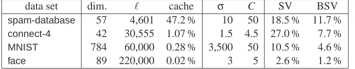
We want to pay special attention to the size of the kernel matrices in comparison to the cache size (see Table 1). The data sets cover a wide range of kernel matrix sizes which fit into the cache by nearly 50 % to only 0.02 %. It is a hopeless approach to adapt the cache size in order to fit larger parts of the kernel matrix into working memory. Because the space requirement for the kernel matrix grows quadratically withℓ, large scale real world problems exceed any physically available cache.
data set dim. ℓ cache σ C SV BSV
spam-database 57 4,601 47.2 % 10 50 18.5 % 11.7 %
connect-4 42 30,555 1.07 % 1.5 4.5 27.0 % 7.7 %
MNIST 784 60,000 0.28 % 3,500 50 10.5 % 4.6 %
face 89 220,000 0.02 % 3 5 2.6 % 1.2 %
Table 1: SVM parameters used in the comparison together with solution statistics. The column “dim.” gives the input space dimension whileℓis the number of training examples. The “cache”-column shows how much of the kernel matrix fits into the kernel cache. The fractions of support vectors and bounded support vectors are denoted by “SV” and “BSV”. These percentage values might slightly differ between the algorithms because of the finite accuracy of the solutions.
4.2 Comparison of Working Set Selection Strategies
We trained SVMs on all data sets presented in the previous section. We monitored the number of iterations and the time until the stopping criterion was met. The results are shown in Table 2. The final target function values f(α∗)are also presented to prove the comparability of the stopping criteria (for the starting state it holds f(α(0)) =0). Indeed, the final values are very close and which algorithm is most accurate depends on the problem.
It becomes clear from the experiments that the LIBSVM-2.71 algorithm performs worst. This is no surprise because it does not take second order information into account. In the following we will concentrate on the comparison of the second order algorithms LIBSVM-2.8 and HMG.
As the smallest problem considered the spam-database consists of 4,601 training examples.
The matrix Q requires about 81 MB of working memory. The cache size of 40 MB should be sufficient when using the shrinking technique. The LIBSVM-2.8 algorithm profits from the fact that the kernel matrix fits into the cache after the first shrinking event. It takes less iterations and (in the mean) the same time per iteration as the HMG algorithm and is thus the fastest in the end.
data set (ℓ) algorithm iterations runtime f(α∗)
LIBSVM-2.71 36,610 11.21 s 27,019.138
spam-database(4,601) LIBSVM-2.8 9,228 8.44 s 27,019.140
HMG 10,563 9.17 s 27,019.140
LIBSVM-2.71 65,167 916 s 13,557.542
connect-4(30,555) LIBSVM-2.8 45,504 734 s 13,557.542
HMG 50,281 633 s 13,557.536
LIBSVM-2.71 185,162 13,657 s 143,199.142
MNIST(60,000) LIBSVM-2.8 110,441 9,957 s 143,199.146
HMG 152,873 7,485 s 143,199.160
LIBSVM-2.71 37,137 14,239 s 15,812.666
face(220,000) LIBSVM-2.8 32,783 14,025 s 15,812.666
HMG 42,303 11,278 s 15,812.664
Table 2: Comparison of the number of iterations of the decomposition algorithm and training times for the different working set selection approaches. In each case the best value is high-lighted. The differences are highly significant (Wilcoxon rank sum test, p<0.001). Addi-tionally, the final value of the objective function showing the comparability of the results is given.
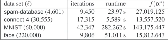
We performed the same experiments with the SVMlightsupport vector machine implementation. The results are summarized in Table 3. We relaxed the stopping condition such that the SVMlight solutions are less accurate than the LIBSVM solutions. Nevertheless, the SVMlight algorithm is slower than the LIBSVM implementation using the SMO algorithm (see Table 2). Please note that according to the numerous implementation differences these experiments do not provide a fair comparison between SMO-like methods and decomposition algorithms using larger working sets.
data set (ℓ) iterations runtime f(α∗)
spam-database(4,601) 9,450 23.97 s 27,019,125
connect-4(30,555) 17,315 5,589 s 13,557.520
MNIST(60,000) 42,347 282,262 s 143,175.447
face(220,000) 9,806 51,011 s 15,812.643
Table 3: Iterations, runtime and objective function value of the SVMlightexperiments with working set size q=10. Because of the enormous runtime, only one trial was conducted for the
4.3 Analysis of Different Parameter Regimes
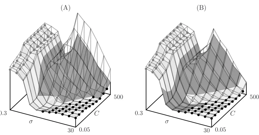
The choice of the regularization parameter C and the parameterσof the Gaussian kernel (6) influ-ence the quadratic problem induced by the data. We analyzed this dependency using grid search on theconnect-4problem. The results are plotted in Figure 6.
All parameter configurations where LIBSVM-2.71 or LIBSVM-2.8 outperformed HMG have one important property in common, namely, that it is a bad idea to reselect an element of the previous working set. This is true when after most iterations both coordinates indexed by the working set are already optimal. This can happen for different reasons:
• Forσ→0 the feature vectors corresponding to the training examples become more and more orthogonal and the quadratic problem
P
becomes (almost) separable.• For increasing values ofσthe example points become more and more similar in the feature space until they are hard to distinguish. This increases the quotient of the largest and smallest eigenvalue of Q. Thus, the solution of
P
is very likely to lie in a corner or on a very low dimensional edge of the box constraining the problem, that is, many of theα∗i end up at the constraints 0 or C. This is even more likely for small values of C.We argue that in practice parameter settings leading to those situations are not really relevant be-cause they tend to produce degenerate solutions. Either almost all examples are selected as support vectors (and the SVM converges to nearest neighbor classification) or the information available are used inefficiently, setting most support vector coefficients to C. Both extremes are usually not in-tended in SVM learning. In our experiments, HMG performs best in the parameter regime giving well generalizing solutions.
4.4 Influence of the Shrinking Algorithm
A shrinking heuristics in a decomposition algorithm tries to predict whether a variableαiwill end up at the box constraint, that is, whether it will take one of the values 0 or C. In this case the variable is fixed at the boundary and the optimization problem is reduced accordingly. Of course, every heuristics can fail and thus when the stopping criterion is met these variables must be reconsidered. The temporary reduction of the problem restricts working set selection algorithms to a subset of possible choices. This may cause more iterations but has the potential to save a lot of runtime.
We repeated our experiments with the LIBSVM shrinking heuristics turned off to reveal the relation between the working set selection algorithms and shrinking, see Table 4. The experiments show that the influence of the shrinking algorithm on the different working set selection policies is highly task dependent. The time saved and even the algorithm for which more time was saved differs from problem to problem. For some problems the differences between the methods increase, for others they decrease. Compared to the experiments with shrinking turned on the results qualitatively remain the same.
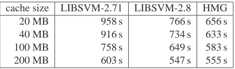
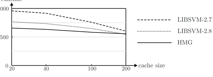
4.5 Influence of the Cache Size