Clustering with Bregman Divergences

Clustering with Bregman Divergences

Arindam Banerjee [email protected]

Srujana Merugu [email protected]

Department of Electrical and Computer Engineering University of Texas at Austin

Austin, TX 78712, USA.

Inderjit S. Dhillon [email protected]

Department of Computer Sciences University of Texas at Austin Austin, TX 78712, USA

Joydeep Ghosh [email protected]

Department of Electrical and Computer Engineering University of Texas at Austin

Austin, TX 78712, USA.

Editor: John Lafferty

Abstract

A wide variety of distortion functions, such as squared Euclidean distance, Mahalanobis distance, Itakura-Saito distance and relative entropy, have been used for clustering. In this paper, we pro-pose and analyze parametric hard and soft clustering algorithms based on a large class of distortion functions known as Bregman divergences. The proposed algorithms unify centroid-based paramet-ric clustering approaches, such as classicalkmeans, the Linde-Buzo-Gray (LBG) algorithm and information-theoretic clustering, which arise by special choices of the Bregman divergence. The algorithms maintain the simplicity and scalability of the classicalkmeansalgorithm, while gener-alizing the method to a large class of clustering loss functions. This is achieved by first posing the hard clustering problem in terms of minimizing the loss in Bregman information, a quantity motivated by rate distortion theory, and then deriving an iterative algorithm that monotonically de-creases this loss. In addition, we show that there is a bijection between regular exponential families and a large class of Bregman divergences, that we call regular Bregman divergences. This result enables the development of an alternative interpretation of an efficient EM scheme for learning mix-tures of exponential family distributions, and leads to a simple soft clustering algorithm for regular Bregman divergences. Finally, we discuss the connection between rate distortion theory and Breg-man clustering and present an information theoretic analysis of BregBreg-man clustering algorithms in terms of a trade-off between compression and loss in Bregman information.

Keywords: clustering, Bregman divergences, Bregman information, exponential families, expectation

maxi-mization, information theory

1. Introduction

cluster representative corresponding to every cluster, such that a well-defined cost function

involv-ing the data and the representatives is minimized. Typically, these clusterinvolv-ing methods come in two flavors: hard and soft. In hard clustering, one obtains a disjoint partitioning of the data such that each data point belongs to exactly one of the partitions. In soft clustering, each data point has a certain probability of belonging to each of the partitions. One can think of hard clustering as a special case of soft clustering where these probabilities only take values 0 or 1. The popularity of parametric clustering algorithms stems from their simplicity and scalability.

Several algorithms for solving particular versions of parametric clustering problems have been developed over the years. Among the hard clustering algorithms, the most well-known is the it-erative relocation scheme for the Euclideankmeansalgorithm (MacQueen, 1967; Jain and Dubes, 1988; Duda et al., 2001). Another widely used clustering algorithm with a similar scheme is the Linde-Buzo-Gray (LBG) algorithm (Linde et al., 1980; Buzo et al., 1980) based on the Itakura-Saito distance, which has been used in the signal-processing community for clustering speech data. The recently proposed information theoretic clustering algorithm (Dhillon et al., 2003) for clustering probability distributions also has a similar flavor.

The observation that for certain distortion functions, e.g., squared Euclidean distance, KL-divergence (Dhillon et al., 2003), Itakura-Saito distance (Buzo et al., 1980) etc., the clustering problem can be solved using appropriatekmeanstype iterative relocation schemes leads to a natu-ral question: what class of distortion functions admit such an iterative relocation scheme where a

global objective function based on the distortion with respect to cluster centroids1is progressively decreased? In this paper, we provide an answer to this question: we show that such a scheme works for arbitrary Bregman divergences. In fact, it can be shown (Banerjee et al., 2005) that such a

sim-ple scheme works only when the distortion is a Bregman divergence. The scope of this result is vast since Bregman divergences include a large number of useful loss functions such as squared loss, KL-divergence, logistic loss, Mahalanobis distance, Itakura-Saito distance, I-divergence, etc.

We pose the hard clustering problem as one of obtaining an optimal quantization in terms of minimizing the loss in Bregman information, a quantity motivated by rate distortion theory. A sim-ple analysis then yields a version of the loss function that readily suggests a natural algorithm to solve the clustering problem for arbitrary Bregman divergences. Partitional hard clustering to min-imize the loss in mutual information, otherwise known as information theoretic clustering (Dhillon et al., 2003), is seen to be a special case of our approach. Thus, this paper unifies several parametric partitional clustering approaches.

Several researchers have observed relationships between Bregman divergences and exponen-tial families (Azoury and Warmuth, 2001; Collins et al., 2001). In this paper, we formally prove an observation made by Forster and Warmuth (2000) that there exists a unique Bregman

diver-gence corresponding to every regular exponential family. In fact, we show that there is a bijection

between regular exponential families and a class of Bregman divergences, that we call regular Breg-man divergences. We show that, with proper representation, the bijection provides an alternative interpretation of a well known efficient EM scheme (Redner and Walker, 1984) for learning mixture models of exponential family distributions. This scheme simplifies the computationally intensive maximization step of the EM algorithm, resulting in a general soft-clustering algorithm for all regu-lar Bregman divergences. We also present an information theoretic analysis of Bregman clustering algorithms in terms of a trade-off between compression and loss in Bregman information.

1.1 Contributions

We briefly summarize the main contributions of this paper:

1. In the context of hard clustering, we introduce the concept of Bregman Information (Sec-tion 3) that measures the minimum expected loss incurred by encoding a set of data points using a constant, where loss is measured in terms of a Bregman divergence. Variance and mutual information are shown to be special cases of Bregman information. Further, we show a close connection between Bregman information and Jensen’s inequality.

2. Hard clustering with Bregman divergences is posed as a quantization problem that involves minimizing loss of Bregman information. We show (Theorem 1 in Section 3) that for any given clustering, the loss in Bregman information is equal to the expected Bregman diver-gence of data points to their respective cluster centroids. Hence, minimizing either of these quantities yields the same optimal clustering.

3. Based on our analysis of the Bregman clustering problem, we present a meta hard clustering algorithm that is applicable to all Bregman divergences (Section 3). The meta clustering algorithm retains the simplicity and scalability ofkmeansand is a direct generalization of all previously known centroid-based parametric hard clustering algorithms.

4. To obtain a similar generalization for the soft clustering case, we show (Theorem 4, Section 4) that there is a uniquely determined Bregman divergence corresponding to every regular ex-ponential family. This result formally proves an observation made by Forster and Warmuth (2000). In particular, in Section 4.3, we show that the log-likelihood of any parametric ex-ponential family is equal to the negative of the corresponding Bregman divergence to the expectation parameter, up to a fixed additive non-parametric function. Further, in Section 4.4, we define regular Bregman divergences using exponentially convex functions and show that there is a bijection between regular exponential families and regular Bregman divergences.

5. Using the correspondence between exponential families and Bregman divergences, we show that the mixture estimation problem based on regular exponential families is identical to a Bregman soft clustering problem (Section 5). Further, we describe an EM scheme to effi-ciently solve the mixture estimation problem. Although this particular scheme for learning mixtures of exponential families was previously known (Redner and Walker, 1984), the Breg-man divergence viewpoint explaining the efficiency is new. In particular, we give a correctness proof of the efficient M-step updates using properties of Bregman divergences.

6. Finally, we study the relationship between Bregman clustering and rate distortion theory (Sec-tion 6). Based on the results in Banerjee et al. (2004a), we observe that the Bregman hard and soft clustering formulations correspond to the “scalar” and asymptotic rate distortion prob-lems respectively, where distortion is measured using a regular Bregman divergence. Further, we show how each of these problems can be interpreted as a trade-off between compression and loss in Bregman information. The information-bottleneck method (Tishby et al., 1999) can be readily derived as a special case of this trade-off.

by upper-case alphabets, e.g., X,Y . The symbolsR,N,ZandRd denote the set of reals, the set of natural numbers, the set of integers and the d-dimensional real vector space respectively. Further,

R₊andR++denote the set of non-negative and positive real numbers. For x,y∈Rd,kxkdenotes

the L2norm, andhx,yidenotes the inner product. Unless otherwise mentioned, log will represent

the natural logarithm. Probability density functions (with respect to the Lebesgue or the counting measure) are denoted by lower case alphabets such as p,q. If a random variable X is distributed

according toν, expectation of functions of X are denoted by EX[·], or by Eν[·]when the random variable is clear from the context. The interior, relative interior, boundary, closure and closed convex hull of a set

X

are denoted by int(

X

), ri(

X

), bd(

X

), cl(

X

)and co(

X

) respectively. The effective domain of a function f , i.e., set of all x such that f(x)<+∞is denoted by dom(f)while the range is denoted by range(f). The inverse of a function f , when well-defined, is denoted by f−1.

2. Preliminaries

In this section, we define the Bregman divergence corresponding to a strictly convex function and present some examples.

Definition 1 (Bregman, 1967; Censor and Zenios, 1998) Letφ:

S

7→R,

S

=dom(φ)be a strictly convex function defined on a convex set

S

⊆Rd _{such that}φ_{is differentiable on ri(}

_S

_{), assumed to} be nonempty. The Bregman divergence d_φ:

S

×ri(

S

)_7→[0,∞)is defined as

d_φ(x,y) =φ(x)₋φ(y)_{− h}x₋y,∇φ(y)_i,

where∇φ(y)represents the gradient vector ofφevaluated at y.

Example 1 Squared Euclidean distance is perhaps the simplest and most widely used Bregman

divergence. The underlying functionφ(x) =_hx,x_iis strictly convex, differentiable onRdand

dφ(x,y) = _hx,x_{i − h}y,y_{i − h}x₋y,∇φ(y)_i = _hx,x_{i − h}y,y_{i − h}x₋y,2y_i = _hx₋y,x₋y_i=_kx₋y_k2.

Example 2 Another widely used Bregman divergence is the KL-divergence. If p is a discrete

prob-ability distribution so that ∑d_j=1pj =1, the negative entropyφ(p) =∑dj=1pjlog2pj is a convex function. The corresponding Bregman divergence is

d_φ(p,q) = d

∑

j=1

pjlog2pj− d

∑

j=1

qjlog2qj− hp−q,∇φ(q)i

= d

∑

j=1

pjlog2pj− d

∑

j=1

qjlog2qj− d

∑

j=1

(pj−qj)(log2qj+log2e)

= d

∑

j=1 pjlog2

pj

qj

−log₂e

d

∑

j=1

(pj−qj)

= KL(p_kq),

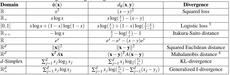
Table 1: Bregman divergences generated from some convex functions.

Domain φ(x) d_φ(x,y) Divergence

R x2 (x−y)2 _{Squared loss}

R+ x log x x log(xy)−(x−y)

[0,1] x log x+ (1−x)log(1−x) x log(_yx) + (1−x)log(1₁−₋x_y) Logistic loss3

R++ −log x xy−log(

x

y)−1 Itakura-Saito distance

R ex ex−ey−(x−y)ey

Rd _kxk2 _kx−yk2 _{Squared Euclidean distance}

Rd _xT_{Ax (x−y)}T_{A(x−y) Mahalanobis distance}4

d-Simplex ∑d_j=1xjlog2xj ∑dj=1xjlog2(

xj

yj) KL-divergence

Rd

+ ∑dj=1xjlog xj ∑dj=1xjlog(

xj yj)−∑

d

j=1(xj−yj) Generalized I-divergence

Example 3 Itakura-Saito distance is another Bregman divergence that is widely used in signal

pro-cessing. If F(ejθ)is the power spectrum2of a signal f(t), then the functionalφ(F) =₋1

2πR−ππ log(F(ejθ))dθ

is convex in F and corresponds to the negative entropy rate of the signal assuming it was generated by a stationary Gaussian process (Palus, 1997; Cover and Thomas, 1991). The Bregman divergence between F(ejθ)and G(ejθ)(the power spectrum of another signal g(t)) is given by

dφ(F,G) = 1 2π

Z π

−π

−log(F(ejθ)) +log(G(ejθ))₋(F(ejθ)₋G(ejθ))

− 1 G(ejθ₎

dθ

= 1

2π Z π

−π

−log

F(ejθ)

G(ejθ₎

+F(e jθ₎

G(ejθ₎−1

dθ,

which is exactly the Itakura-Saito distance between the power spectra F(ejθ)and G(ejθ) and can also be interpreted as the I-divergence (Csisz´ar, 1991) between the generating processes under the assumption that they are equal mean, stationary Gaussian processes (Kazakos and Kazakos, 1980).

Table 1 contains a list of some common convex functions and their corresponding Bregman diver-gences. Bregman divergences have several interesting and useful properties, such as non-negativity, convexity in the first argument, etc. For details see Appendix A.

3. Bregman Hard Clustering

In this section, we introduce a new concept called the Bregman information of a random variable based on ideas from Shannon’s rate distortion theory. Then, we motivate the Bregman hard cluster-ing problem as a quantization problem that involves minimizcluster-ing the loss in Bregman information and show its equivalence to a more direct formulation, i.e., the problem of finding a partitioning and a representative for each of the partitions such that the expected Bregman divergence of the data

2. Note that F(·)is a function and it is possible to extend the notion of Bregman divergences to the space of func-tions (Csisz´ar, 1995; Gr¨unwald and Dawid, 2004).

3. For x∈ {0,1}(Bernoulli) and y∈(0,1)(posterior probability for x=1), we have x log(x

y) + (1−x)log(

1−x

1−y) = log(1+exp(−f(x)g(y))), i.e., the logistic loss with f(x) =2x−1 and g(y) =log(₁₋y_y).

points from their representatives is minimized. We then present a clustering algorithm that gen-eralizes the iterative relocation scheme ofkmeansto monotonically decrease the loss in Bregman information.

3.1 Bregman Information

The dual formulation of Shannon’s celebrated rate distortion problem (Cover and Thomas, 1991; Gr¨unwald and Vit´anyi, 2003) involves finding a coding scheme with a given rate, i.e., average number of bits per symbol, such that the expected distortion between the source random variable and the decoded random variable is minimized. The achieved distortion is called the distortion

rate function, i.e., the infimum distortion achievable for a given rate. Now consider a random

variable X that takes values in a finite set

X

=_{xi}n_i=1⊂

S

⊆Rd(

S

is convex) following a discrete probability measure ν. Let the distortion be measured by a Bregman divergence d_φ. Consider a simple encoding scheme that represents the random variable by a constant vector s, i.e., codebook size is one, or rate is zero. The solution to the rate-distortion problem in this case is the trivial assignment. The corresponding distortion-rate function is given by E_ν[d_φ(X,s)]that depends on the choice of the representative s and can be optimized by picking the right representative. We call this optimal distortion-rate function the Bregman information of the random variable X for the Bregman divergence d_φand denote it by I_φ(X), i.e.,

I_φ(X) = min

s∈ri(S)Eν[dφ(X,s)] =s∈minri(S)

n

∑

i=1

νid_φ(xi,s). (1)

The optimal vector s that achieves the minimal distortion will be called the Bregman representative or, simply the representative of X . The following theorem states that this representative always ex-ists, is uniquely determined and, surprisingly, does not depend on the choice of Bregman divergence. In fact, the minimizer is just the expectation of the random variable X .

Proposition 1 Let X be a random variable that take values in

X

=_{xi}in=1⊂

S

⊆Rd following a positive probability measureνsuch that Eν[X]_∈ri(

S

).5 Given a Bregman divergence dφ:

S

_×

ri(

S

)_7→[0,∞), the problem

min

s∈ri(S)Eν[dφ(X,s)] (2)

has a unique minimizer given by s†_=µ=E ν[X].

Proof The function we are trying to minimize is J_φ(s) =E_ν[d_φ(X,s)] =∑n_i=1νid_φ(xi,s). Since

µ=E_ν[X]_∈ri(S), the objective function is well-defined atµ. Now,_∀s_∈ri(

S

),

J_φ(s)₋J_φ(µ) = n

∑

i=1

νid_φ(xi,s)− n

∑

i=1

νid_φ(xi,µ)

= φ(µ)₋φ(s)₋

*

n

∑

i=1

νixi−s,∇φ(s)

+

+

*

n

∑

i=1

νixi−µ,∇φ(µ)

+

= φ(µ)₋φ(s)_{− h}µ₋s,∇φ(s)_i = d_φ(µ,s)_≥0,

with equality only when s=µby the strict convexity ofφ(Appendix A, Property 1). Hence,µis the unique minimizer of Jφ.

Note that the minimization in (2) is with respect to the second argument of d_φ. Proposition 1 is somewhat surprising since Bregman divergences are not necessarily convex in the second argument as the following example demonstrates.

Example 4 Considerφ(x) =∑3

j=1x3j defined onR3+so that dφ(x,s) =∑3j=1(x3j−s3j−3(xj−sj)s2j). For the random variable X distributed uniformly over the set

X

=_{(1,1,1),(2,2,2),(3,3,3),(4,4,4),

(5,5,5)_},

E[d_φ(X,s)] =135+2

3

∑

j=1 s3_j−9

3

∑

j=1 s2_j ,

which is clearly not convex in s since the Hessian∇2Jφ(s) =diag(12s₋18)is not positive definite. However, J_φ(s)is uniquely minimized by s= (3,3,3), i.e., the expectation of the random variable

X .

Interestingly, the converse of Proposition 1 is also true, i.e., for all random variables X , if E[X] minimizes the expected distortion of X to a fixed point for a smooth distortion function F(x,y)(see Appendix B for details), then F(x,y)has to be a Bregman divergence (Banerjee et al., 2005). Thus, Bregman divergences are exhaustive with respect to the property proved in Proposition 1.

Using Proposition 1, we can now give a more direct definition of Bregman information as fol-lows:

Definition 2 Let X be a random variable that takes values in

X

=_{xi}n_i=1⊂

S

following a proba-bility measureν. Letµ=E_ν[X] =∑n

i=1νixi∈ri(

S

)and let dφ:

S

×ri(

S

)7→[0,∞)be a Bregman divergence. Then the Bregman Information of X in terms of d_φis defined as

I_φ(X) =E_ν[d_φ(X,µ)] = n

∑

i=1

νidφ(xi,µ).

Example 5 (Variance) Let

X

=_{xi}n_i=1 be a set in Rd, and consider the uniform measure, i.e., νi= 1

n, over

X

. The Bregman information of X with squared Euclidean distance as the Bregman divergence is given by

Iφ(X) = n

∑

i=1

νidφ(xi,µ) = 1

n

n

∑

i=1

kxi−µk2, which is just the sample variance.

Example 6 (Mutual Information) By definition, the mutual information I(U ;V)between two dis-crete random variables U and V with joint distribution_{{p(ui,vj)}n_i=1}m_j=1is given by

I(U ;V) = n

∑

i=1

m

∑

j=1

p(ui,vj)log

p(ui,vj)

p(ui)p(vj) =

n

∑

i=1 p(ui)

m

∑

j=1

p(vj|ui)log

p(vj|ui)

p(vj)

= n

∑

i=1

Consider a random variable Zuthat takes values in the set of probability distributions

Z

u={p(V|ui)}ni=1

following the probability measure_{νi_}n_i=1=_{p(ui)}n_i=1over this set. The mean (distribution) of Zu is given by

µ=Eν[p(V|u)] = n

∑

i=1

p(ui)p(V|ui) = n

∑

i=1

p(ui,V) =p(V).

Hence,

I(U ;V) = n

∑

i=1

νidφ(p(V_|ui),µ) =Iφ(Zu),

i.e., mutual information is the Bregman information of Zuwhen dφis the KL-divergence. Similarly, for a random variable Zvthat takes values in the set of probability distributions

Z

v={p(U|vj)}m_j=1 following the probability measure_{νj_}m_j=1=_{p(vj)}m_j=1over this set, one can show that I(U ;V) =

I_φ(Zv). The Bregman information of Zuand Zvcan also be interpreted as the Jensen-Shannon diver-gence of the sets

Z

uand

Z

v(Dhillon et al., 2003).

Example 7 The Bregman information corresponding to Itakura-Saito distance also has a useful

interpretation. Let

F

=_{Fi}ni=1be a set of power spectra corresponding to n different signals, and

letνbe a probability measure on

F

. Then, the Bregman information of a random variable F that takes values in

F

followingν, with Itakura-Saito distance as the Bregman divergence, is given by

Iφ(F) = n

∑

i=1

νidφ(Fi,F¯) = n

∑

i=1

νi 2π Z π −π −log

Fi(ejθ) ¯

F(ejθ₎

+Fi(e jθ₎

¯

F(ejθ₎−1

dθ

= ₋ 1

2π Z π

−π

n

∑

i=1

νilog

Fi(ejθ) ¯

F(ejθ₎

dθ,

where ¯F is the marginal average power spectrum. Based on the connection between the

corre-sponding convex function φand the negative entropy of Gaussian processes (Cover and Thomas, 1991; Palus, 1997), it can be shown that the Bregman information I_φ(F) is the Jensen-Shannon divergence of the generating processes under the assumption that they are equal mean, stationary Gaussian processes. Further, consider a n-class signal classification problem where each class of signals is assumed to be generated by a certain Gaussian process. Now, if Pe(t)is the optimal Bayes error for this classification problem averaged upto time t, then Pe(t)is bounded above and below by functions of the Chernoff coefficient B(t)(Kazakos and Kazakos, 1980) of the generating Gaussian processes. The asymptotic value of this Chernoff coefficient as t tends to ∞is a function of the Bregman information of F, i.e.,

lim

t→∞B(t) =exp(− 1 2Iφ(F)). and is directly proportional to the optimal Bayes error.

3.1.1 JENSEN’SINEQUALITY AND BREGMANINFORMATION

An alternative interpretation of Bregman information can also be made in terms of Jensen’s inequal-ity (Cover and Thomas, 1991). Given any convex functionφ, for any random variable X , Jensen’s inequality states that

A direct calculation using the definition of Bregman information shows that (Banerjee et al., 2004b)

E[φ(X)]₋φ(E[X]) (=a) E[φ(X)]₋φ(E[X])₋E[_hX₋E[X],∇φ(E[X])_i]

(b)

= E[φ(X)₋φ(E[X])_{− h}X−E[X],∇φ(E[X])_i] = E[d_φ(X,E[X])] = I_φ(X) _≥ 0,

where (a) follows since the last term is 0, and (b) follows from the linearity of expectation. Thus the difference between the two sides of Jensen’s inequality is exactly equal to the Bregman information.

3.2 Clustering Formulation

Let X be a random variable that takes values in

X

=_{xi}n_i=1following the probability measureν. When X has a large Bregman information, it may not suffice to encode X using a single represen-tative since a lower quantization error may be desired. In such a situation, a natural goal is to split the set

X

into k disjoint partitions _{

X

h}k_h=1, each with its own Bregman representative, such that a random variable M over the partition representatives serves as an appropriate quantization of X . Let

M

=_{µh}k_h=1 denote the set of representatives, andπ={πh}k_h=1 withπh=∑xi∈Xhνi denote

the induced probability measure on

M

. Then the induced random variable M takes values in

M

followingπ.

The quality of the quantization M can be measured by the expected Bregman divergence be-tween X and M, i.e., EX,M[dφ(X,M)]. Since M is a deterministic function of X , the expectation is actually over the distribution of X , so that

EX[dφ(X,M)] = k

∑

h=1x

∑

i∈Xh

νidφ(xi,µh) = k

∑

h=1

πh

∑

xi∈Xh

νi

πhdφ(xi,µh) = Eπ[Iφ(Xh)],

where Xh is the random variable that takes values in the partition

X

h following a probability dis-tribution νi

πh, and Iφ(Xh)is the Bregman information of Xh. Thus, the quality of the quantization is

equal to the expected Bregman information of the partitions.

An alternative way of measuring the quality of the quantization M can be formulated from an information theoretic viewpoint. In information-theoretic clustering (Dhillon et al., 2003), the quality of the partitioning is measured in terms of the loss in mutual information resulting from the quantization of the original random variable X . Extending this formulation, we can measure the quality of the quantization M by the loss in Bregman information due to the quantization, i.e., by

Iφ(X)₋Iφ(M). For k=n, the best choice is of course M=X with no loss in Bregman information.

For k=1, the best quantization is to pick Eν[X]with probability 1, incurring a loss of Iφ(X). For intermediate values of k, the solution is less obvious.

Interestingly the two possible formulations outlined above turn out to be identical (see Theo-rem 1 below). We choose the information theoretic viewpoint to pose the problem, since we will study the connections of both the hard and soft clustering problems to rate distortion theory in Sec-tion 6. Thus we define the Bregman hard clustering problem as that of finding a partiSec-tioning of

X

, or, equivalently, finding the random variable M, such that the loss in Bregman information due to quantization, L_φ(M) =I_φ(X)₋I_φ(M), is minimized. Typically, clustering algorithms assume a uniform measure, i.e.,νi=1

Theorem 1 Let X be a random variable that takes values in

X

=_{xi}in=1⊂

S

⊆Rd following the positive probability measureν. Let_{

X

h}k_h=1be a partitioning of

X

and letπh=∑xi∈Xhνi be the

induced measureπon the partitions. Let Xhbe the random variable that takes values in

X

hfollowing

νi

πh for xi∈

X

h, for h=1, . . . ,k. Let

M

={µh}

k

h=1withµh∈ri(

S

)denote the set of representatives of_{Xh}k_h=1, and M be a random variable that takes values in

M

followingπ. Then,

L_φ(M) = I_φ(X)₋I_φ(M) = E_π[I_φ(Xh)] = k

∑

h=1

πh

∑

xi∈Xh

νi

πh dφ(xi,µh).

Proof By definition,

I_φ(X) = n

∑

i=1

νid_φ(xi,µ) = k

∑

h=1xi

∑

∈Xh

νid_φ(xi,µ)

= k

∑

h=1xi

∑

∈Xh

νi{φ(xi)−φ(µ)− hxi−µ,∇φ(µ)i}

= k

∑

h=1xi

∑

∈Xh

νi{φ(xi)−φ(µh)− hxi−µh,∇φ(µh)i+hxi−µh,∇φ(µh)i

+φ(µh)−φ(µ)− hxi−µh+µh−µ,∇φ(µ)i}

= k

∑

h=1xi

∑

∈Xh

νi

d_φ(xi,µh) +dφ(µh,µ) +hxi−µh,∇φ(µh)−∇φ(µ)i

= k

∑

h=1

πh

∑

xi∈Xh

νi

πhdφ(xi,µh) + k

∑

h=1xi

∑

∈Xh

νid_φ(µh,µ)

+ k

∑

h=1

πh

∑

xi∈Xh

νi

πhhxi−µh,∇φ(µh)−∇φ(µ)i

= k

∑

h=1

πhIφ(Xh) + k

∑

h=1

πhdφ(µh,µ) + k

∑

h=1

πh

*

∑

xi∈Xh

νi

πhxi−µh,∇φ(µh)−∇φ(µ)

+

= Eπ[Iφ(Xh)] +Iφ(M),

since∑_xi∈Xh νi

πhxi=µh.

Note that Iφ(X)can be interpreted as the “total Bregman information”, and Iφ(M)can be interpreted as the “between-cluster Bregman information” since it is a measure of divergence between the clus-ter representatives, while Lφ(M)can be interpreted as the “within-cluster Bregman information”. Thus Theorem 1 states that the total Bregman information equals the sum of the within-cluster Bregman information and between-cluster Bregman information. This is a generalization of the corresponding result for squared Euclidean distances (Duda et al., 2001).

Using Theorem 1, the Bregman clustering problem of minimizing the loss in Bregman informa-tion can be written as

min

M Iφ(X)−Iφ(M)

=min M

k

∑

h=1x

∑

i∈Xh

νidφ(xi,µh)

!

Algorithm 1 Bregman Hard Clustering

Input: SetX ={xi}ni=1⊂S⊆Rd, probability measureνoverX, Bregman divergence dφ:S×ri(S)7→R, number of clusters k.

Output:M†_{, local minimizer of L}

φ(M) =∑kh=1∑xi∈Xhνidφ(xi,µh)whereM ={µh}

k

h=1, hard partitioning {Xh}kh=1ofX.

Method:

Initialize_{µh}kh=1withµh∈ri(S)(one possible initialization is to chooseµh∈ri(S)at random) repeat

{The Assignment Step_} SetXh←/0, 1≤h≤k for i=1 to n do

Xh←Xh∪ {xi}

where h=h†(xi) =argmin h0

dφ(xi,µh0)

end for

{The Re-estimation Step_}

for h=1 to k do

πh←∑xi∈Xhνi

µh←_π1_h∑xi∈Xhνixi

end for until convergence

return M†_{← {µ}

h}k_h=1

Thus, the loss in Bregman information is minimized if the set of representatives

M

is such that the expected Bregman divergence of points in the original set

X

to their corresponding representatives is minimized. We shall investigate the relationship of this formulation to rate distortion theory in detail in Section 6.

3.3 Clustering Algorithm

The objective function given in (3) suggests a natural iterative relocation algorithm for solving the Bregman hard clustering problem (see Algorithm 1). It is easy to see that classical kmeans, the LBG algorithm (Buzo et al., 1980) and the information theoretic clustering algorithm (Dhillon et al., 2003) are special cases of Bregman hard clustering for squared Euclidean distance, Itakura-Saito distance and KL-divergence respectively. The following propositions prove the convergence of the Bregman hard clustering algorithm.

Proposition 2 The Bregman hard clustering algorithm (Algorithm 1) monotonically decreases the loss function in (3).

Proof Let_{

X

_h(t)}k

h=1be the partitioning of

X

after the tthiteration and let

M

(t)={µ

(t)

h }kh=1be the

corresponding set of cluster representatives. Then,

Lφ(M(t)) = k

∑

h=1_x

∑

i∈X(

t)

h

νidφ(xi,µ(_ht))

(a)

≥

k

∑

h=1_x

∑

i∈X(

t)

h

νidφ(xi,µ(_ht†)_(x

i))

(b)

≥

k

∑

h=1_x

∑

i∈X(

t+1)

h

where (a) follows from the assignment step, and (b) follows from the re-estimation step and Propo-sition 1. Note that if equality holds, i.e., if the loss function value is equal at consecutive iterations, then the algorithm will terminate.

Proposition 3 The Bregman hard clustering algorithm (Algorithm 1) terminates in a finite number of steps at a partition that is locally optimal, i.e., the total loss cannot be decreased by either (a) the assignment step or by (b) changing the means of any existing clusters.

Proof The result follows since the algorithm monotonically decreases the objective function value,

and the number of distinct clusterings is finite.

In addition to local optimality, the Bregman hard clustering algorithm has the following inter-esting properties.

Exhaustiveness: The Bregman hard clustering algorithm with cluster centroids as optimal

repre-sentatives works for all Bregman divergences and only for Bregman divergences since the arithmetic mean is the best predictor only for Bregman divergences (Banerjee et al., 2005). However, it is possible to have a similar alternate minimization based clustering algorithm for distance functions that are not Bregman divergences, the primary difference being that the optimal cluster representative, when it exists, will no longer be the arithmetic mean or the expectation. Theconvex-kmeansclustering algorithm (Modha and Spangler, 2003) and the generalizations of the LBG algorithm (Linde et al., 1980) are examples of such alternate minimization schemes where a (unique) representative exists because of convexity.

Linear Separators: For all Bregman divergences, the partitions induced by the Bregman hard

clustering algorithm are separated by hyperplanes. In particular, the locus of points that are equidistant to two fixed points µ1,µ2 in terms of a Bregman divergence is given by

X

= {x_|d_φ(x,µ1) =dφ(x,µ2)}, i.e., the set of points,

{x_{| h}x,∇φ(µ2)−∇φ(µ1)i= (φ(µ1)− hµ1,∇φ(µ1)i)−(φ(µ2)− hµ2,∇φ(µ2)i)},

which corresponds to a hyperplane.

Scalability: The computational complexity of each iteration of the Bregman hard clustering

algo-rithm is linear in the number of data points and the number of desired clusters for all Bregman divergences, which makes the algorithm scalable and appropriate for large clustering prob-lems.

Applicability to mixed data types: The Bregman hard clustering algorithm is applicable to mixed

data types that are commonly encountered in machine learning. One can choose different convex functions that are appropriate and meaningful for different subsets of the features. The Bregman divergence corresponding to a convex combination of the component convex functions can then be used to cluster the data.

4. Relationship with Exponential Families

family distribution. Later, we make this relation more precise by establishing a bijection between regular exponential families and regular Bregman divergences. The correspondence will be used to develop the Bregman soft clustering algorithm in Section 5. To present our results, we first review some background information on exponential families and Legendre duality in Sections 4.1 and 4.2 respectively.

4.1 Exponential Families

Consider a measurable space(Ω,

B

)where

B

is a σ-algebra on the setΩ. Let t be a measurable mapping from Ω to a set

T

⊆Rd_{, where}

_T

_{may be discrete (e.g.,}

_T

_{⊂N). Let p}

0:

T

7→R+

be any function such that if (Ω,

B

) is endowed with a measure dP0(ω) = p0(t(ω))dt(ω), then

R

ω∈ΩdP0(ω)<∞. The measure P0 is absolutely continuous with respect to the Lebesgue

mea-sure dt(ω). When

T

is a discrete set, dt(ω)is the counting measure and P0is absolutely continuous

with respect to the counting measure.6

Now, t(ω)is a random variable from(Ω,

B

,P0)to(

T

,σ(

T

)), whereσ(

T

)denotes theσ-algebra generated by

T

. LetΘbe defined as the set of all parametersθ_∈Rdfor which

Z

ω∈Ωexp(hθ,t(ω)i)dP0(ω)<∞.

Based on the definition ofΘ, it is possible to define a functionψ:Θ7→Rsuch that

ψ(θ) =log

_Z

ω∈Ωexp(hθ,t(ω)i)dP0(ω)

. (4)

A family of probability distributions

F

ψparameterized by a d-dimensional vectorθ_∈Θ_⊆Rd_such that the probability density functions with respect to the measure dt(ω)can be expressed in the form

f(ω;θ) =exp(_hθ,t(ω)_{i −}ψ(θ))p0(t(ω)) (5)

is called an exponential family with natural statistic t(ω), natural parameterθand natural

param-eter space Θ. In particular, if the components of t(ω) are affinely independent, i.e., @ non-zero

a_∈Rd such that_ha,t(ω)_i=c (a constant)_∀ω_∈Ω, then this representation is said to be minimal.7

For a minimal representation, there exists a unique probability density f(ω;θ)for every choice of

θ_∈Θ(Wainwright and Jordan, 2003).

F

ψ is called a full exponential family of order d in such a case. In addition, if the parameter spaceΘ is open, i.e., Θ=int(Θ), then

F

ψ is called a regular

exponential family.

It can be easily seen that if x_∈Rddenotes the natural statistic t(ω), then the probability density function g(x;θ)(with respect to the appropriate measure dx) given by

g(x;θ) =exp(_hθ,x_{i −}ψ(θ))p0(x) (6)

is such that f(ω;θ)/g(x;θ)does not depend onθ. Thus, x is a sufficient statistic (Amari and Na-gaoka, 2001) for the family, and in fact, can be shown (Barndorff-Nielsen, 1978) to be minimally

6. For conciseness, we abuse notation and continue to use the Lebesgue integral sign even for counting measures. The integral in this case actually denotes a sum overT. Further, the use of absolute continuity in the context of counting measure is non-standard. We say the measure P0is absolutely continuous with respect to the counting measure µcif P0(E) =0 for every set with µc(E) =0, where E is a discrete set.

sufficient. For instance, the natural statistic for the one-dimensional Gaussian distributions denoted by f(ω;σ,µ) =√1

2πσexp(−

(ω−µ)2

2σ2 )is given by x= [ω,ω2]and the corresponding natural parameter turns out to beθ= [_σµ2,−2σ12], which can be easily verified to be minimally sufficient. For our anal-ysis, it is convenient to work with the minimal natural sufficient statistic x and hence, we redefine regular exponential families in terms of the probability density of x_∈Rd, noting that the original probability space can actually be quite general.

Definition 3 A multivariate parametric family

F

ψof distributions_{p(ψ,θ)|θ∈Θ=int(Θ) =dom(ψ)⊆

Rd_{}is called a regular exponential family if each probability density is of the form}

p(ψ,θ)(x) =exp(hx,θi −ψ(θ))p0(x), ∀x∈Rd,

where x is a minimal sufficient statistic for the family.

The functionψ(θ)is known as the log partition function or the cumulant function corresponding to the exponential family. Given a regular exponential family

F

ψ, the log-partition functionψ is uniquely determined up to a constant additive term. It can be shown (Barndorff-Nielsen, 1978) that Θ is a non-empty convex set inRd andψ is a convex function. In fact, it is possible to prove a stronger result that characterizesψin terms of a special class of convex functions called Legendre functions, which are defined below.

Definition 4 (Rockafellar (1970)) Letψbe a proper, closed8_{convex function with}Θ_=int(dom(ψ_)).

The pair(Θ,ψ)is called a convex function of Legendre type or a Legendre function if the following properties are satisfied:

(L1) Θis non-empty,

(L2) ψis strictly convex and differentiable onΘ,

(L3) _∀θb∈bd(Θ), lim

θ_→θbk

∇ψ(θ)_{k →}∞whereθ_∈Θ.

Based on this definition, we now state a critical property of the cumulant function of any regular exponential family.

Lemma 1 Letψbe the cumulant function of a regular exponential family with natural parameter spaceΘ=dom(ψ). Thenψ is a proper, closed convex function with int(Θ) =Θand(Θ,ψ) is a convex function of Legendre type.

The above result directly follows from Theorems 8.2, 9.1 and 9.3 of Barndorff-Nielsen (1978).

4.2 Expectation Parameters and Legendre Duality

Consider a d-dimensional real random vector X distributed according to a regular exponential family density p_(ψ,θ)specified by the natural parameterθ_∈Θ. The expectation of X with respect to p_(ψ,θ), also called the expectation parameter, is given by

µ=µ(θ) =Ep(ψ,θ)[X] =

Z

Rdxp(ψ,θ)(x)dx. (7)

It can be shown (Barndorff-Nielsen, 1978; Amari, 1995) that the expectation and natural parameters have a one-one correspondence with each other and span spaces that exhibit a dual relationship. To specify the duality more precisely, we first define conjugate functions.

Definition 5 (Rockafellar (1970)) Letψbe a real-valued function onRd. Then its conjugate

func-tionψ∗is given by

ψ∗_{(t) = sup}

θ_∈dom(ψ){h

t,θ_{i −}ψ(θ)_}. (8)

Further, ifψ is a proper closed convex function, ψ∗ is also a proper closed convex function and ψ∗∗_=ψ.

Whenψis strictly convex and differentiable overΘ=int(dom(ψ)), we can obtain the uniqueθ†

that corresponds to the supremum in (8) by setting the gradient of_ht,θ_{i −}ψ(θ)to zero, i.e., ∇(_ht,θ_{i −}ψ(θ))_|θ=θ† =0 ⇒ t=∇ψ(θ†). (9) The strict convexity of ψ implies that ∇ψ is monotonic and it is possible to define the inverse function(∇ψ)−1_:Θ∗_{7→Θ, whereΘ}∗_=int(dom(ψ∗_{)). If the pair (Θ,ψ) is of Legendre type, then}

it can be shown (Rockafellar, 1970) that (Θ∗_,ψ∗_{) is also of Legendre type, and(Θ,ψ)and(Θ}∗_,ψ∗₎

are called Legendre duals of each other. Further, the gradient mappings are continuous and form a bijection between the two open setsΘandΘ∗. The relation between(Θ,ψ)and(Θ∗,ψ∗)result is formally stated below.

Theorem 2 (Rockafellar (1970)) Letψbe a real-valued proper closed convex function with con-jugate functionψ∗. LetΘ=int(dom(ψ))andΘ∗=int(dom(ψ∗)). If(Θ,ψ)is a convex function of Legendre type, then

(i) (Θ∗,ψ∗)is a convex function of Legendre type,

(ii) (Θ,ψ)and(Θ∗,ψ∗)are Legendre duals of each other,

(iii) The gradient function∇ψ:Θ_7→Θ∗is a one-to-one function from the open convex setΘonto the open convex setΘ∗,

(iv) The gradient functions∇ψ,∇ψ∗are continuous, and∇ψ∗= (∇ψ)−1_.

Let us now look at the relationship between the natural parameterθand the expectation parameterµ

defined in (7). Differentiating the identityR

p(ψ,θ)(x)dx=1 with respect toθgives usµ=µ(θ) =

∇ψ(θ), i.e., the expectation parameterµis the image of the natural parameterθunder the gradient mapping∇ψ. Letφbe defined as the conjugate ofψ, i.e.,

φ(µ) =sup

θ∈Θ{h

µ,θ_{i −}ψ(θ)_}. (10)

Since(Θ,ψ)is a convex function of Legendre type (Lemma 1), the pairs(Θ,ψ)and(int(dom(φ)),φ) are Legendre duals of each other from Theorem 2, i.e.,φ=ψ∗ and int(dom(φ)) =Θ∗. Thus, the mappings between the dual spaces int(dom(φ))andΘare given by the Legendre transformation

µ(θ) =∇ψ(θ) and θ(µ) =∇φ(µ). (11)

Further, the conjugate functionφcan be expressed as

4.3 Exponential Families and Bregman Divergences

We are now ready to explicitly state the formal connection between exponential families of distri-butions and Bregman divergences. It has been observed in the literature that exponential families and Bregman divergences have a close relationship that can be exploited for several learning prob-lems. In particular, Forster and Warmuth (2000)[Section 5.1] remarked that the log-likelihood of the density of an exponential family distribution p(ψ,θ) can be written as the sum of the negative

of a uniquely determined Bregman divergence d_φ(x,µ)and a function that does not depend on the distribution parameters. In our notation, this can be written as

log(p_(ψ,θ)(x)) =₋d_φ(x,µ(θ)) +log(b_φ(x)), (13)

whereφis the conjugate function ofψandµ=µ(θ) =∇ψ(θ)is the expectation parameter cor-responding toθ. The result was later used by Collins et al. (2001) to extend PCA to exponential families. However, as we explain below, a formal proof is required to show that (13) holds for all instances x of interest. We focus on the case when p(ψ,θ)is a regular exponential family.

To get an intuition of the main result, observe that the log-likelihood of any exponential family, considering only the parametric terms, can be written as

hx,θ_{i −}ψ(θ) = (_hµ,θ_{i −}ψ(θ)) +_hx₋µ,θ_i

= φ(µ) +_hx₋µ,∇φ(µ)_i,

from (11) and (12), where µ_∈int(dom(φ)). Therefore, for any x _∈dom(φ), θ_∈Θ, and µ_∈

int(dom(φ)), one can write

hx,θ_{i −}ψ(θ) = ₋dφ(x,µ) +φ(x).

Then considering the density of an exponential family with respect to the appropriate measure dx, we have

log(p(ψ,θ)(x)) = hx,θi −ψ(θ) +log p0(x) = −dφ(x,µ) +log(bφ(x)),

where b_φ(x) =exp(φ(x))p0(x).

Thus (13) follows directly from Legendre duality for x_∈dom(φ). However, for (13) to be useful, one would like to ensure that it is true for all individual “instances” x that can be drawn following the exponential distribution p(ψ,θ). Let Iψdenote the set of such instances. Establishing (13) can be

tricky for all x_∈Iψsince the relationship between Iψand dom(φ)is not apparent. Further, there are distributions for which the instances space I_ψand the expectation parameter space int(dom(φ))are disjoint, as the following example shows.

Example 8 A Bernoulli random variable X takes values in _{0,1_} such that p(X =1) =q and p(X=0) =1₋q, for some q_∈[0,1]. The instance space for X is just I_ψ=_{0,1_}. The cumulant function for X isψ(θ) =log(1+exp(θ))withΘ=R(see Table 2). A simple calculation shows that the conjugate functionφ(µ) =µ log µ+ (1₋µ)log(1₋µ), _∀µ_∈(0,1). Sinceφis a closed function, we obtainφ(µ) =0 for µ_{∈ {}0,1_}by taking limits. Thus, the effective domain ofφis[0,1]and µ=q,

whereas the expectation parameter space is given by int(dom(φ)) = (0,1). Hence the instance space

In this particular case, since the “instances” lie within dom(φ), the relation (13) does hold for all

x_∈Iψ. However, it remains to be shown that Iψ⊆dom(φ)for all regular exponential family distri-butions.

In order to establish such a result for all regular exponential family distributions, we need to formally define the set of instances Iψ. If the measure P0is absolutely continuous with respect to the

counting measure, then x_∈I_ψif p_(ψ,θ)(x)>0. On the other hand, if P0is absolutely continuous with

respect to the Lebesgue measure, then x∈Iψif all sets with positive Lebesgue measure that contain

x have positive probability mass. A closer look reveals that the set of instances Iψis independent of the choice ofθ. In fact, I_ψis just the support of P0and can be formally defined as follows.

Definition 6 Let Iψdenote the set of instances that can be drawn following p(ψ,θ)(x). Then, x0∈Iψ

if_∀I such that x0_∈I andR

Idx>0, we have R

IdP0(x)>0, where P0is as defined in Section 4.1; also see footnote 6.

The following theorem establishes the crucial result that the set of instances Iψis always a subset of dom(φ).

Theorem 3 Let I_ψ be the set of instances as in Definition 6. Then, I_{ψ ⊆}dom(φ) where φis the conjugate function ofψ.

The above result follows from Theorem 9.1 and related results in Barndorff-Nielsen (1978). We have included the proof in Appendix C.

We are now ready to formally show that there is a unique Bregman divergence corresponding to every regular exponential family distribution. Note that, by Theorem 3, it is sufficient to establish the relationship for all x_∈dom(φ).

Theorem 4 Let p(ψ,θ)be the probability density function of a regular exponential family

distribu-tion. Letφbe the conjugate function ofψso that(int(dom(φ)),φ)is the Legendre dual of(Θ,ψ). Let θ_∈Θbe the natural parameter andµ_∈int(dom(φ))be the corresponding expectation parameter. Let dφbe the Bregman divergence derived fromφ. Then p(ψ,θ)can be uniquely expressed as

p(ψ,θ)(x) =exp(−dφ(x,µ))bφ(x), ∀x∈dom(φ) (14)

where b_φ: dom(φ)_7→R₊is a uniquely determined function.

Proof For all x_∈dom(φ), we have

p(ψ,θ)(x) = exp(hx,θi −ψ(θ))p0(x)

= exp(φ(µ) +_hx₋µ,∇φ(µ)_i)p0(x) (using (11) and (12))

= exp(_−{φ(x)₋φ(µ)_{− h}x₋µ,∇φ(µ)_i}+φ(x))p0(x)

= exp(₋d_φ(x,µ))b_φ(x),

where bφ(x) =exp(φ(x))p0(x)).

from any of these conjugate functions will be identical since constant additive terms do not change the corresponding Bregman divergence (Appendix A, Property 4). The Legendre duality between φandψalso ensures that no two exponential families correspond to the same Bregman divergence, i.e., the mapping is one-to-one. Further, since p(ψ,θ)(x)is well-defined on dom(φ), and the

corre-sponding dφ(x,µ)is unique, the function bφ(x) =exp(dφ(x,µ))p(ψ,θ)(x)is uniquely determined.

4.4 Bijection with Regular Bregman Divergences

From Theorem 4 we note that every regular exponential family corresponds to a unique and dis-tinct Bregman divergence (one-to-one mapping). Now, we investigate whether there is a regular exponential family corresponding to every choice of Bregman divergence (onto mapping).

For regular exponential families, the cumulant functionψas well as its conjugateφare convex functions of Legendre type. Hence, for a Bregman divergence generated from a convex functionφ to correspond to a regular exponential family, it is necessary thatφbe of Legendre type. Further, it is necessary that the Legendre conjugate ψ ofφto be C∞, since cumulant functions of regular exponential families are C∞. However, it is not clear if these conditions are sufficient. Instead, we provide a sufficiency condition using exponentially convex functions (Akhizer, 1965; Ehm et al., 2003), which are defined below.

Definition 7 A function f :Θ_7→R++,Θ⊆Rdis called exponentially convex if the kernel Kf(α,β) =

f(α+β), withα+β_∈Θ, satisfies

n

∑

i=1

n

∑

j=1

Kf(θi,θj)uiu¯j≥0

for any set_{θ1,_···,θn} ⊆Θwithθi+θj∈Θ, ∀i,j, and{u1,···,un} ⊂C( ¯uj denotes the complex conjugate of uj), i.e, the kernel Kf is positive semi-definite.

Although it is well known that the logarithm of an exponentially convex function is a convex func-tion (Akhizer, 1965), we are interested in the case where the logarithm is strictly convex with an open domain. Using this class of exponentially convex functions, we now define a class of Bregman divergences called regular Bregman divergences.

Definition 8 Let f :Θ_7→R++be a continuous exponentially convex function such thatΘis open

andψ(θ) =log(f(θ))is strictly convex. Letφbe the conjugate function ofψ. Then we say that the Bregman divergence d_φderived fromφis a regular Bregman divergence.

We will now prove that there is a bijection between regular exponential families and regular Bregman divergences. The crux of the argument relies on results in harmonic analysis connecting positive definiteness to integral transforms (Berg et al., 1984). In particular, we use a result due to Devinatz (1955) that relates exponentially convex functions to Laplace transforms of bounded non-negative measures.

represented as

f(θ) = Z

x_∈Rdexp(hx,θi)dν(x) (15)

is that f is continuous and exponentially convex.

We also need the following result to establish the bijection.

Lemma 2 Letψbe the cumulant of an exponential family with base measure P0and natural pa-rameter spaceΘ_⊆Rd. Then, if P0is concentrated on an affine subspace ofRdthenψis not strictly convex.

Proof Let P0(x) be concentrated on an affine subspace S={x∈Rd|hx,bi=c} for some b∈Rd

and c∈R. Let I=_{θ_|θ=αb,α_∈R_}. Then, for anyθ=αb∈I, we havehx,θ_i=αc∀x∈S and

the cumulant is given by

ψ(θ) = log

Z

x_∈Rdexp(hx,θi)dP0(x)

= log

Z

x_∈Sexp(hx,

θ_i)dP0(x)

= log

Z

x∈S

exp(αc)dP0(x)

= log(exp(αc)P0(S)) = αc+log(P0(S))

= _hx0,θ_i+log(P0(S)),

for any x0∈S, implying thatψis not strictly convex.

There are two parts to the proof leading to the bijection result. Note that we have already established in Theorem 4 that there is a unique Bregman divergence corresponding to every exponential family distribution. In the first part of the proof, we show that these Bregman divergences are regular (one-to-one). Then we show that there exists a unique regular exponential family determined by every regular Bregman divergence (onto).

Theorem 6 There is a bijection between regular exponential families and regular Bregman diver-gences.

Proof First we prove the ‘one-to-one’ part, i.e., there is a regular Bregman divergence corresponding

to every regular exponential family F_ψ with cumulant functionψ and natural parameter spaceΘ. Since

F

ψis a regular exponential family, there exists a non-negative bounded measure νsuch that for allθ_∈Θ,

1 =

Z

x∈Rdexp(hx,θi −ψ(θ))dν(x)

⇒ exp(ψ(θ)) = Z

x∈Rdexp(hx,θi)dν(x).

Thus, from Theorem 5, exp(ψ(θ))is a continuous exponentially convex function with the open set Θas its domain. Further, being the cumulant of a regular exponential family,ψis strictly convex. Therefore, the Bregman divergence d_φ derived from the conjugate function φ of ψ is a regular Bregman divergence.

the conjugate ofφ. Since dφis a regular Bregman divergence, by Definition 8,ψis strictly convex with dom(ψ) =Θbeing an open set. Further, the function exp(ψ(θ))is a continuous, exponentially convex function. From Theorem 5, there exists a unique non-negative bounded measure νthat satisfies (15). SinceΘis non-empty, we can choose some fixed b∈Θso that

exp(ψ(b)) = Z

x∈Rdexp(hx,bi)dν(x)

and so dP0(x) =exp(hx,bi −ψ(b))dν(x)is a probability density function. The set of allθ∈Rdfor

which

Z

x∈Rdexp(hx,θi)dP0(x)<∞

is same as the set _{θ _∈Rd_|exp(ψ(θ+b)₋ψ(b))<∞_}=_{θ_∈Rd_|θ+b_∈Θ_} which is just a translated version ofΘitself. For anyθsuch thatθ+b∈Θ, we have

Z

x∈Rdexp(hx,θ+bi −ψ(θ+b))dν(x) =1.

Hence, the exponential family

F

ψconsisting of densities of the form

p_(ψ,θ)(x) =exp(_hx,θ_{i −}ψ(θ))

with respect to the measureνhasΘas its natural parameter space andψ(θ)as the cumulant function. Sinceψis strictly convex onΘ, it follows from Lemma 2 that the measure P0is not concentrated

in an affine subspace ofRd, i.e., x is a minimal statistic for

F

ψ. Therefore, the exponential family generated by P0and x is full. SinceΘis also open, it follows that

F

ψis a regular exponential family.

Finally we show that the family is unique. Since only d_φis given, the generating convex function could be ¯φ(x) =φ(x) +_hx,a_i+c for a_∈Rd and a constant c_∈R. The corresponding conjugate function ¯ψ(θ) =ψ(θ₋a)₋c differs fromψonly by a constant. Hence, the exponential family is exactly

F

ψ. That completes the proof.

4.5 Examples

Table 2 shows the various functions of interest for some popular exponential families. We now look at two of these distributions in detail and obtain the corresponding Bregman divergences.

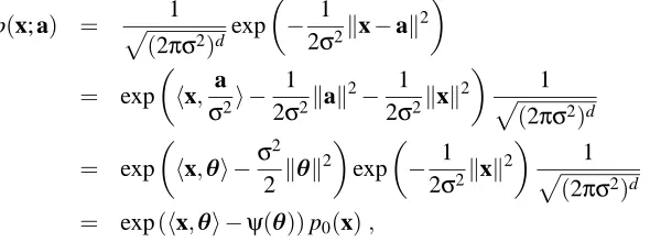
Example 9 The most well-known exponential family is that of Gaussian distributions, in particular

uniform variance, spherical Gaussian distributions with densities of the form

p(x; a) =p 1

(2πσ2₎dexp

−_2σ12kx−ak 2