Diffusion Kernels on Statistical Manifolds

Diffusion Kernels on Statistical Manifolds

John Lafferty [email protected]

Guy Lebanon [email protected]

School of Computer Science Carnegie Mellon University Pittsburgh, PA 15213 USA

Editor: Tommi Jaakkola

Abstract

A family of kernels for statistical learning is introduced that exploits the geometric structure of statistical models. The kernels are based on the heat equation on the Riemannian manifold defined by the Fisher information metric associated with a statistical family, and generalize the Gaussian kernel of Euclidean space. As an important special case, kernels based on the geometry of multi-nomial families are derived, leading to kernel-based learning algorithms that apply naturally to discrete data. Bounds on covering numbers and Rademacher averages for the kernels are proved using bounds on the eigenvalues of the Laplacian on Riemannian manifolds. Experimental results are presented for document classification, for which the use of multinomial geometry is natural and well motivated, and improvements are obtained over the standard use of Gaussian or linear kernels, which have been the standard for text classification.

Keywords: kernels, heat equation, diffusion, information geometry, text classification

1. Introduction

The use of Mercer kernels for transforming linear classification and regression schemes into nonlin-ear methods is a fundamental idea, one that was recognized nonlin-early in the development of statistical learning algorithms such as the perceptron, splines, and support vector machines (Aizerman et al., 1964; Kimeldorf and Wahba, 1971; Boser et al., 1992). The resurgence of activity on kernel methods in the machine learning community has led to the further development of this important technique, demonstrating how kernels can be key components in tools for tackling nonlinear data analysis problems, as well as for integrating data from multiple sources.

collection (Joachims, 2000). While such a representation has proven to be effective, the statistical justification of such a transform of categorical data into Euclidean space is unclear.

Motivated by this need for kernel methods that can be applied to discrete, categorical data, Kondor and Lafferty (2002) propose the use of discrete diffusion kernels and tools from spectral graph theory for data represented by graphs. In this paper, we propose a related construction of kernels based on the heat equation. The key idea in our approach is to begin with a statistical family that is natural for the data being analyzed, and to represent data as points on the statistical manifold associated with the Fisher information metric of this family. We then exploit the geometry of the statistical family; specifically, we consider the heat equation with respect to the Riemannian structure given by the Fisher metric, leading to a Mercer kernel defined on the appropriate function spaces. The result is a family of kernels that generalizes the familiar Gaussian kernel for Euclidean space, and that includes new kernels for discrete data by beginning with statistical families such as the multinomial. Since the kernels are intimately based on the geometry of the Fisher information metric and the heat or diffusion equation on the associated Riemannian manifold, we refer to them here as information diffusion kernels.

One apparent limitation of the discrete diffusion kernels of Kondor and Lafferty (2002) is the difficulty of analyzing the associated learning algorithms in the discrete setting. This stems from the fact that general bounds on the spectra of finite or even infinite graphs are difficult to obtain, and research has concentrated on bounds on the first eigenvalues for special families of graphs. In contrast, the kernels we investigate here are over continuous parameter spaces even in the case where the underlying data is discrete, leading to more amenable spectral analysis. We can draw on the considerable body of research in differential geometry that studies the eigenvalues of the geometric Laplacian, and thereby apply some of the machinery that has been developed for analyzing the generalization performance of kernel machines in our setting.

Although the framework proposed is fairly general, in this paper we focus on the application of these ideas to text classification, where the natural statistical family is the multinomial. In the simplest case, the words in a document are modeled as independent draws from a fixed multino-mial; non-independent draws, corresponding to n-grams or more complicated mixture models are also possible. For n-gram models, the maximum likelihood multinomial model is obtained simply as normalized counts, and smoothed estimates can be used to remove the zeros. This mapping is then used as an embedding of each document into the statistical family, where the geometric frame-work applies. We remark that the perspective of associating multinomial models with individual documents has recently been explored in information retrieval, with promising results (Ponte and Croft, 1998; Zhai and Lafferty, 2001).

We present detailed experiments for text classification, using both the WebKB and Reuters data sets, which have become standard test collections. Our experimental results indicate that the multi-nomial information diffusion kernel performs very well empirically. This improvement can in part be attributed to the role of the Fisher information metric, which results in points near the boundary of the simplex being given relatively more importance than in the flat Euclidean metric. Viewed differently, effects similar to those obtained by heuristically designed term weighting schemes such as inverse document frequency are seen to arise automatically from the geometry of the statistical manifold.

The remaining sections are organized as follows. In Section 2 we review the relevant concepts that are required from Riemannian geometry, including the heat kernel for a general Riemannian manifold and its parametrix expansion. In Section 3 we define the Fisher metric associated with a statistical manifold of distributions, and examine in some detail the special cases of the multinomial and spherical normal families; the proposed use of the heat kernel or its parametrix approximation on the statistical manifold is the main contribution of the paper. Section 4 derives bounds on cov-ering numbers and Rademacher averages for various learning algorithms that use the new kernels, borrowing results from differential geometry on bounds for the geometric Laplacian. Section 5 describes the results of applying the multinomial diffusion kernels to text classification, and we conclude with a discussion of our results in Section 6.

2. The Heat Kernel

In this section we review the basic properties of the heat kernel on a Riemannian manifold, together with its asymptotic expansion, the parametrix. The heat kernel and its parametrix expansion contains a wealth of geometric information, and indeed much of modern differential geometry, notably index theory, is based upon the use of the heat kernel and its generalizations. The fundamental nature of the heat kernel makes it a natural candidate to consider for statistical learning applications. An excellent introductory account of this topic is given by Rosenberg (1997), and an authoritative reference for spectral methods in Riemannian geometry is Schoen and Yau (1994). In Appendix A we review some of the elementary concepts from Riemannian geometry that are required, as these concepts are not widely used in machine learning, in order to help make the paper more self-contained.

2.1 The Heat Kernel

The Laplacian is used to model how heat will diffuse throughout a geometric manifold; the flow is governed by the following second order differential equation with initial conditions

∂f

∂t −∆f = 0 f(x,0) = f0(x).

The value f(x,t)describes the heat at location x at time t, beginning from an initial distribution of heat given by f0(x) at time zero. The heat or diffusion kernel Kt(x,y) is the solution to the heat

equation f(x,t)with initial condition given by Dirac’s delta functionδy. As a consequence of the linearity of the heat equation, the heat kernel can be used to generate the solution to the heat equation with arbitrary initial conditions, according to

f(x,t) =

Z

M

As a simple special case, consider heat flow on the circle, or one-dimensional sphere M=S1, with the metric inherited from the Euclidean metric onR2_{. Parameterizing the manifold by angle}θ_, and letting f(θ,t) =∑∞_j=0aj(t)cos(jθ)be the discrete cosine transform of the solution to the heat equation, with initial conditions given by aj(0) =aj, it is seen that the heat equation leads to the equation

∞

∑

j=0

d

dtaj(t) +j

2_a

j(t)

cos(jθ) =0,

which is easily solved to obtain aj(t) =e−j

2_t

and therefore f(θ,t) =∑∞_j=0aje−j

2_t

cos(jθ). As the time parameter t gets large, the solution converges to f(θ,t)_−→a0, which is the average value of

f ; thus, the heat diffuses until the manifold is at a uniform temperature. To express the solution in terms of an integral kernel, note that by the Fourier inversion formula

f(θ,t) = ∞

∑

j=0

hf,ei jθie−j2tei jθ

= 1

2π Z

S1 ∞

∑

j=0

e−j2tei jθe−i jφf0(φ)dφ,

thus expressing the solution as f(θ,t) =R

S1Kt(θ,φ)f0(φ)dφfor the heat kernel Kt(φ,θ) =

1 2π

∞

∑

j=0

e−j2tcos(j(θ₋φ)).

This simple example shows several properties of the general solution of the heat equation on a (compact) Riemannian manifold; in particular, note that the eigenvalues of the kernel scale asλj∼ e−j2/d where the dimension in this case is d=1.

When M=R_{, the heat kernel is the familiar Gaussian kernel, so that the solution to the heat} equation is expressed as

f(x,t) =√1

4πt Z

R

e−(x−y)

2

4t _f0(_y)_dy,

and it is seen that as t_−→∞, the heat diffuses out “to infinity” so that f(x,t)_−→0.

When M is compact, the Laplacian has discrete eigenvalues 0=µ0<µ1≤µ2··· with

corre-sponding eigenfunctionsφisatisfying∆φi=−µiφi. When the manifold has a boundary, appropriate

boundary conditions must be imposed in order for∆ to be self-adjoint. Dirichlet boundary

con-ditions set φi|_∂M =0 and Neumann boundary conditions require ∂φ

i

∂ν

_∂

M =0 whereνis the outer normal direction. The following theorem summarizes the basic properties for the kernel of the heat equation on M; we refer to Schoen and Yau (1994) for a proof.

Theorem 1 Let M be a complete Riemannian manifold. Then there exists a function K_∈C∞(R_+× M_×M), called the heat kernel, which satisfies the following properties for all x,y _∈M, with Kt(·,·) =K(t,·,·)

1. Kt(x,y) =Kt(y,x)

3.

∆−_∂∂t

Kt(x,y) =0

4. Kt(x,y) =R_MKt₋s(x,z)Ks(z,y)dz for any s>0 .

If in addition M is compact, then Ktcan be expressed in terms of the eigenvalues and eigenfunctions of the Laplacian as Kt(x,y) =∑∞i=0e−µitφi(x)φi(y).

Properties 2 and 3 imply that Kt(x,y)solves the heat equation in x, starting from a point heat source at y. It follows that et∆_f

0(x) = f(x,t) =

R

MKt(x,y)f0(y)dy solves the heat equation with

initial conditions f(x,0) = f0(x), since

∂f(x,t) ∂t =

Z

M

∂Kt(x,y)

∂t f0(y)dy

=

Z

M

∆Kt(x,y)f0(y)dy

= ∆

Z

M

Kt(x,y)f0(y)dy

= ∆f(x,t),

and limt→0f(x,t) =

R

Mlimt→0Kt(x,y)dy= f0(x). Property 4 implies that et∆es∆=e(t+s)∆, which

has the physically intuitive interpretation that heat diffusion for time t is the composition of heat diffusion up to time s with heat diffusion for an additional time t₋s. Since et∆is a positive operator,

Z

M Z

M

Kt(x,y)g(x)g(y)dx dy = Z

M

f(x)et∆g(x)dx

= _hg,et∆g_{i ≥}0.

Thus Kt(x,y) is positive-definite. In the compact case, positive-definiteness follows directly from the expansion Kt(x,y) =∑∞i=0e−µitφi(x)φi(y), which shows that the eigenvalues of Kt as an integral operator are e−µit_{. Together, these properties show that K}

t defines a Mercer kernel.

The heat kernel Kt(x,y)is a natural candidate for measuring the similarity between points be-tween x,y_∈M, while respecting the geometry encoded in the metric g. Furthermore it is, unlike the geodesic distance, a Mercer kernel—a fact that enables its use in statistical kernel machines. When this kernel is used for classification, as in our text classification experiments presented in Section 5, the discriminant function yt(x) =∑iαiyiKt(x,xi)can be interpreted as the solution to the heat equation with initial temperature y0(xi) =αiyion labeled data points xi, and initial temperature y0(x) =0 elsewhere.

2.1.1 THEPARAMETRIXEXPANSION

For most geometries, there is no closed form solution for the heat kernel. However, the short time behavior of the solutions can be studied using an asymptotic expansion called the parametrix expansion. In fact, the existence of the heat kernel, as asserted in the above theorem, is most directly proven by first showing the existence of the parametrix expansion. In Section 5 we will employ the first-order parametrix expansion for text classification.

Recall that the heat kernel on flat n-dimensional Euclidean space is given by

KEuclid

t (x,y) = (4πt)−

n

2_exp

−kx−yk 2

4t

wherekx−yk2_=∑n

i=1|xi−yi|2is the squared Euclidean distance between x and y. The parametrix expansion approximates the heat kernel locally as a correction to this Euclidean heat kernel. To begin the definition of the parametrix, let

Pt(m)(x,y) = (4πt)−

n

2exp

−d

2_(x,y)

4t

(ψ0(x,y) +ψ1(x,y)t+_···+ψm(x,y)tm) (1)

for currently unspecified functionsψk(x,y), but where d2(x,y)now denotes the square of the geodesic distance on the manifold. The idea is to obtainψk recursively by solving the heat equation approxi-mately to order tm, for small diffusion time t.

Let r=d(x,y)denote the length of the radial geodesic from x to y_∈Vxin the normal coordinates defined by the exponential map. For any functions f(r)and h(r)of r, it can be shown that

∆f = d 2_f

dr2 +

d log√det g dr

d f dr

∆(f h) = f∆h+h∆f+2d f dr

dh dr.

Starting from these basic relations, some calculus shows that

∆−_∂∂_t

P_t(m)= (tm∆ψm) (4πt)−

n

2_exp

−r 2

4t

(2)

whenψkare defined recursively as

ψ0 =

√

det g rn₋1

−1

2

(3)

ψk = r−kψ0 Z r

0 ψ

−1

0 (∆φk−1)sk−1ds for k>0. (4)

With this recursive definition of the functionsψk, the expansion (1), which is defined only locally, is then extended to all of M_×M by smoothing with a “cut-off function”η, with the specification thatη:R_{+−→[0,1]is C}∞_and

η(r) =

(

0 r≥1

1 r_≤c

for some constant 0<c<1. Thus, the order-m parametrix is defined as

Kt(m)(x,y) =η(d(x,y))P

(m)

t (x,y).

As suggested by equation (2), Kt(m) is an approximate solution to the heat equation, and satisfies Kt(x,y) =Kt(m)(x,y)+O(tm)for x and y sufficiently close; in particular, the parametrix is not unique. For further details we refer to (Schoen and Yau, 1994; Rosenberg, 1997).

While the parametrix K_t(m) is not in general positive-definite, and therefore does not define a Mercer kernel, it is positive-definite for t sufficiently small. In particular, define the function f(t) =

3. Diffusion Kernels on Statistical Manifolds

We now proceed to the main contribution of the paper, which is the application of the heat kernel constructions reviewed in the previous section to the geometry of statistical families, in order to obtain kernels for statistical learning.

Under some mild regularity conditions, general parametric statistical families come equipped with a canonical geometry based on the Fisher information metric. This geometry has long been recognized (Rao, 1945), and there is a rich line of research in statistics, with threads in machine learning, that has sought to exploit this geometry in statistical analysis; see Kass (1989) for a survey and discussion, or the monographs by Kass and Vos (1997) and Amari and Nagaoka (2000) for more extensive treatments. The basic properties of the Fisher information metric are reviewed in Appendix B.

We remark that in spite of the fundamental nature of the geometric perspective in statistics, many researchers have concluded that while it occasionally provides an interesting alternative in-terpretation, it has not contributed new results or methods that cannot be obtained through more conventional analysis. However in the present work, the kernel methods we propose can, arguably, be motivated and derived only through the geometry of statistical manifolds.1

The following two basic examples illustrate the geometry of the Fisher information metric and the associated diffusion kernel it induces on a statistical manifold. The spherical normal family corresponds to a manifold of constant negative curvature, and the multinomial corresponds to a manifold of constant positive curvature. The multinomial will be the most important example that we develop, and we report extensive experiments with the resulting kernels in Section 5.

3.1 Diffusion Kernels for Gaussian Geometry

Consider the statistical family given by F=_{p(_·|θ)_}θ∈Θ where θ= (µ,σ) and p(_·|(µ,σ)) =

N

n−1), the Gaussian having mean µ∈Rn−1 and varianceσ2In−1, withσ>0. Thus, Θ=

Rn−1_×R_{+. A derivation of the Fisher information metric for this family is given in Appendix B.1,} where it is shown that under coordinates defined byθ0_i=µifor 1≤i≤n−1 andθ0n=

p

2(n₋1)σ, the Fisher information matrix is given by

gi j(θ0) = 1

σ2δi j.

Thus, the Fisher information metric givesΘ=Rn−1_×R_{+ the structure of the upper half plane in} hyperbolic space. The distance minimizing or geodesic curves in hyperbolic space are straight lines or circles orthogonal to the mean subspace.

In particular, the univariate normal density has hyperbolic geometry. As a generalization in this 2-dimensional case, any location-scale family of densities is seen to have hyperbolic geometry (Kass and Vos, 1997). Such families have densities of the form

p(x_|(µ,σ)) = 1 σf

x₋µ

σ

where(µ,σ)_∈R_×R_{+and f :}R_→R_.

0 0.1 0.2 0.3 0.4 0.5 0.6 0.7 0.8 0.9 1 0 0.1 0.2 0.3 0.4 0.5 0.6 0.7 0.8 0.9 1

0 0.1 0.2 0.3 0.4 0.5 0.6 0.7 0.8 0.9 1 0 0.1 0.2 0.3 0.4 0.5 0.6 0.7 0.8 0.9 1

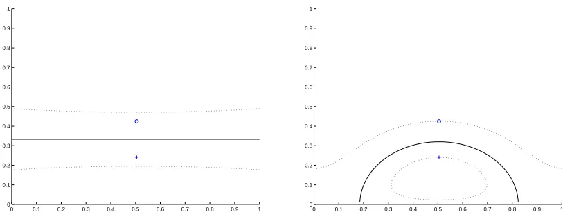
Figure 1: Example decision boundaries for a kernel-based classifier using information diffusion kernels for spherical normal geometry with d=2 (right), which has constant negative curvature, compared with the standard Gaussian kernel for flat Euclidean space (left). Two data points are used, simply to contrast the underlying geometries. The curved decision boundary for the diffusion kernel can be interpreted statistically by noting that as the variance decreases the mean is known with increasing certainty.

The heat kernel on the hyperbolic space Hn _{has the following explicit form (Grigor’yan and} Noguchi, 1998). For odd n=2m+1 it is given by

Kt(x,x0) =

(₋1)m 2mπm

1

√

4πt

1 sinh r ∂ ∂r m exp

−m2t₋r

2

4t

, (5)

and for even n=2m+2 it is given by

Kt(x,x0) =

(₋1)m 2mπm

√

2

√

4πt3

1 sinh r

∂ ∂r

mZ ∞

r s exp

−(2m+41)2t−

s2

4t

√

cosh s₋cosh r ds, (6)

where r=d(x,x0)is the geodesic distance between the two points inHn_{. If only the mean}θ_{=µ is} unspecified, then the associated kernel is the standard Gaussian RBF kernel.

A possible use for this kernel in statistical learning is where data points are naturally represented as sets. That is, suppose that each data point is of the form x=_{x1,x2, . . .xm} where xi ∈Rn−1. Then the data can be represented according to the mapping which sends each group of points to the corresponding Gaussian under the MLE: x7→(_bµ(x),σ(b x))where bµ(x) = 1

m∑ixi andσ(b x)2=

1

m∑i(xi−bµ(x))2.

In Figure 3.1 the diffusion kernel for hyperbolic spaceH2_{is compared with the Euclidean space}

Gaussian kernel. The curved decision boundary for the diffusion kernel makes intuitive sense, since as the variance decreases the mean is known with increasing certainty.

Note that we can, in fact, consider M as a manifold with boundary by allowing σ_≥0 to be

3.2 Diffusion Kernels for Multinomial Geometry

We now consider the statistical family of the multinomial over n+1 outcomes, given by F=

{p(_·|θ)_}θ∈Θ where θ= (θ1,θ2, . . . ,θn) withθi∈(0,1)and∑ni=1θi<1. The parameter space Θ is the open n-simplex

P

To compute the metric, let x= (x1,x2, . . . ,xn+1)denote one draw from the multinomial, so that

xi∈ {0,1}and∑ixi=1. The log-likelihood and its derivatives are then given by

log p(x|θ) =

n+1

∑

i=1

xilogθi

∂log p(x_|θ)

∂θi

= xi θi

∂2_{log p(x|θ)} ∂θi∂θj

= ₋xi θ2

i

δi j.

Since

P

i=1 uiei, v=∑in=+11viei. Note that due to the constraint

∑n+1

i=1θi=1, the sum of the n+1 components of a tangent vector must be zero. A basis for TθM is

n

e1= (1,0, . . . ,0,−1)>,e2= (0,1,0, . . . ,0,−1)>, . . . ,en= (0,0, . . . ,0,1,−1)>

o

.

Using the definition of the Fisher information metric in equation (10) we then compute

hu,v_iθ = ₋

n+1

∑

i=1

n+1

∑

j=1

uivjEθ

_∂2

log p(x_|θ)

∂θi∂θj

= ₋

n+1

∑

i=1

uiviE

−xi/θ2i

=

n+1

∑

i=1

uivi

θi

.

While geodesic distances are difficult to compute in general, in the case of the multinomial information geometry we can easily compute the geodesics by observing that the standard Euclidean metric on the surface of the positive n-sphere is the pull-back of the Fisher information metric on the simplex. This relationship is suggested by the form of the Fisher information given in equation (10).

To be concrete, the transformation F(θ1, . . . ,θn+1) = (2√θ1, . . . ,2√θn+1)is a diffeomorphism

of the n-simplex

P

S

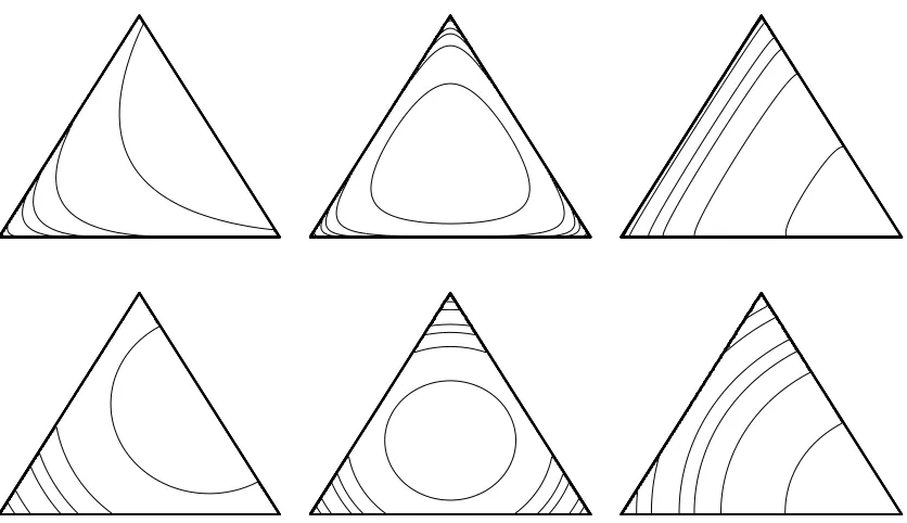
Figure 2: Equal distance contours on

P

∑n+1

i=1viei, the pull-back of the Fisher information metric through F−1is h_θ(u,v) = g_θ2_/4 F_∗−1

n+1

∑

k=1

ukek,F_∗−1 n+1

∑

l=1

vlel

!

=

n+1

∑

k=1

n+1

∑

l=1

ukvlg_θ2_/4(F_∗−1e_k,F_∗−1e_l)

=

n+1

∑

k=1

n+1

∑

l=1

ukvl

∑

4

θ2

i

(F_∗−1ek)i(F_∗−1el)i

=

n+1

∑

k=1

n+1

∑

l=1

ukvl

∑

4

θ2

i

θkδki 2

θlδli 2

=

n+1

∑

i=1

uivi.

Since the transformation F :(

P

S

n ,h)is an isometry, the geodesic distance d(θ,θ0)on

P

S

n connecting F(θ)and F(θ0). These shortest curves are portions of great circles—the intersection of a two dimensional plane and

S

d(θ,θ0) =2 arccos n+1

∑

i=1

q

θiθ0_i

!

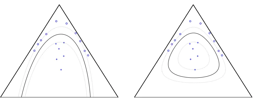
Figure 3: Example decision boundaries using support vector machines with information diffusion kernels for trinomial geometry on the 2-simplex (top right) compared with the standard Gaussian kernel (left).

In Appendix B we recall the connection between the Kullback-Leibler divergence and the in-formation distance. In the case of the multinomial family, there is also a close relationship with the Hellinger distance. In particular, it can easily be shown that the Hellinger distance

dH(θ,θ0) =

s

∑

i

p

θi−

q

θ0

i

2

is related to d(θ,θ0)by

dH(θ,θ0) =2 sin d(θ,θ0)/4

.

Thus, asθ0→θ, dHagrees with 1₂d to second order: dH(θ,θ0) =

1 2d(θ,θ

0_{) +O(d}3_(θ,θ0₎₎

The Fisher information metric places greater emphasis on points near the boundary, which is expected to be important for text problems, which typically have sparse statistics. Figure 2 shows equal distance contours on

P

While the spherical geometry has been derived as the information geometry for a finite multi-nomial, the same geometry can be used non-parametrically for an arbitrary subset of probability measures, leading to spherical geometry in a Hilbert space (Dawid, 1977).

3.2.1 THEMULTINOMIALDIFFUSIONKERNEL

Unlike the explicit expression for the Gaussian geometry discussed above, there is not an explicit form for the heat kernel on the sphere, nor on the positive orthant of the sphere. We will therefore resort to the parametrix expansion to derive an approximate heat kernel for the multinomial.

as defined by the exponential map. As we have just derived, this results in the following parametrix for the multinomial family:

P_t(m)(θ,θ0) = (4πt)−n2exp −arccos

2₍√_θ·√_θ0)

t

!

ψ0(θ,θ0) +_···+ψm(θ,θ0)tm

.

The first-order expansion is thus obtained as

Kt(0)(θ,θ0) =η(d(θ,θ0))P

(0)

t (θ,θ0).

Now, for the n-sphere it can be shown that the functionψ0of (3), which is the leading order correc-tion of the Gaussian kernel under the Fisher informacorrec-tion metric, is given by

ψ0(r) =

√

det g rn₋1

−1

2

=

sin r r

−(n−21)

= 1+(n−1)

12 r

2₊(n−1)(5n−1)

1440 r

4_+O(r6₎

(Berger et al., 1971). Thus, the leading order parametrix for the multinomial diffusion kernel is

Pt(0)(θ,θ0) = (4πt)−

n

2_exp

−_4t1d2(θ,θ0)

sin d(θ,θ0)

d(θ,θ0₎

₋(n−1) 2

.

In our experiments we approximate this kernel further as

P_t(0)(θ,θ0) = (4πt)−n2exp

−1

t arccos

2₍√_θ·√_θ0)

by appealing to the asymptotic expansion in (8) and the explicit form of the distance given in (7); note that (sin r/r)−n blows up for large r. In Figure 3 the kernel (3.2.1) is compared with the standard Euclidean space Gaussian kernel for the case of the trinomial model, d=2, using an SVM classifier.

3.2.2 ROUNDING THESIMPLEX

The case of multinomial geometry poses some technical complications for the analysis of diffusion kernels, due to the fact that the open simplex is not complete, and moreover, its closure is not a dif-ferentiable manifold with boundary. Thus, it is not technically possible to apply several results from differential geometry, such as bounds on the spectrum of the Laplacian, as adopted in Section 4. We now briefly describe a technical “patch” that allows us to derive all of the needed analytical results, without sacrificing in practice any of the methodology that has been derived so far.

Let∆n=

P

boundary since the boundary has edges and corners. In other words, local charts ϕ: U _→Rn+

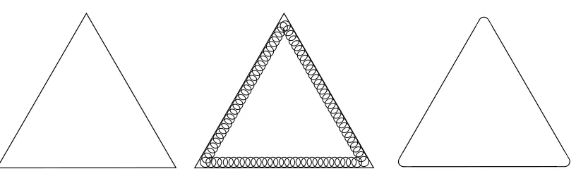
Figure 4: Rounding the simplex. Since the closed simplex is not a manifold with boundary, we

carry out a “rounding” procedure to remove edges and corners. Theδ-rounded simplex

is the closure of the union of allδ-balls lying within the open simplex.

obtain a subset that forms a compact manifold with boundary, and that closely approximates the original simplex.

Forδ>0, let B_δ(x) =_{y_|kx₋y_k<δ_}denote the open Euclidean ball of radiusδcentered at x. Denote by C_δ(

P

P

C_δ(

P

P

P

Finally, let

P

P

P

P

B_δ(x).

Theδ-rounded simplex∆δ_nis then defined as the closure∆δ_n=

P

The rounding procedure that yields ∆δ₂ is suggested by Figure 4. Note that in general theδ -rounded simplex∆δ_nwill contain points with a single, but not more than one component having zero probability. The set∆δ_nforms a compact manifold with boundary, and its image under the isometry F :(

P

S

Whenever appealing to results for compact manifolds with boundary in the following, it will be tacitly assumed that the above rounding procedure has been carried out in the case of the multi-nomial. From a theoretical perspective this enables the use of bounds on spectra of Laplacians for manifolds of non-negative curvature. From a practical viewpoint it requires only smoothing the probabilities to remove zeros.

4. Spectral Bounds on Covering Numbers and Rademacher Averages

on Rademacher averages may be obtained by plugging in the spectral bounds from differential ge-ometry. The primary conclusion that is drawn from these analyses is that from the point of view of generalization error bounds, diffusion kernels behave essentially the same as the standard Gaussian kernel.

4.1 Covering Numbers

We begin by recalling the main result of Guo et al. (2002), modifying their notation slightly to conform with ours. Let M_⊂Rd_{be a compact subset of d-dimensional Euclidean space, and suppose} that K : M_×M_−→R_{is a Mercer kernel. Denote by}λ1_≥λ2_{≥ ··· ≥0 the eigenvalues of K, that is,} of the mapping f _7→R

MK(·,y)f(y)dy, and letψj(·)denote the corresponding eigenfunctions. We assume that CKdef=sup_jψj

_∞<∞.

Given m points xi_∈M, the kernel hypothesis class for x=_{xi}with weight vector bounded by R is defined as the collection of functions on x given by

F

whereΦ(·)is the mapping from M to feature space defined by the Mercer kernel, andh·,_·iandk·k

denote the corresponding Hilbert space inner product and norm. It is of interest to obtain uniform bounds on the covering numbers

N

F

F

in the metric induced by the norm_kf_k∞,x=maxi=1,...,m|f(xi)|.

Theorem 2 (Guo et al., 2002) Given an integer n_∈N_{, let jn}∗_{denote the smallest integer j for which}

λj+1<

_λ1

···λj n2

1

j

and define

ε∗

n=6CKR

v u u t_j∗_n

_λ1

···λj∗

n

n2

1

j∗

n

+ ∞

∑

i=j∗

n

λi.

Then sup_{xi}∈Mm

N

F

To apply this result, we will obtain bounds on the indices j∗_nusing spectral theory in Riemannian geometry.

Theorem 3 (Li and Yau, 1980) Let M be a compact Riemannian manifold of dimension d with non-negative Ricci curvature, and let 0<µ1≤µ2≤ ··· denote the eigenvalues of the Laplacian

with Dirichlet boundary conditions. Then

c1(d)

j V

2

d

≤ µj ≤ c2(d)

j+1 V

2

d

Note that the manifold of the multinomial model (afterδ-rounding) satisfies the conditions of this theorem. Using these results we can establish the following bounds on covering numbers for information diffusion kernels. We assume Dirichlet boundary conditions; a similar result can be proven for Neumann boundary conditions. We include the constant V =vol(M)and diffusion coef-ficient t in order to indicate how the bounds depend on the geometry.

Theorem 4 Let M be a compact Riemannian manifold, with volume V , satisfying the conditions of Theorem 3. Then the covering numbers for the Dirichlet heat kernel Kt on M satisfy

log

N

F

V

td2

logd+22

1

ε

. (8)

Proof By the lower bound in Theorem 3, the Dirichlet eigenvalues of the heat kernel Kt(x,y), which

are given byλj=e−tµj, satisfy logλj≤ −tc1(d)

j V 2 d . Thus,

−1_jlog

_λ1

···λj n2

≥ tc_j1

j

∑

i=1

i V 2 d +2

jlog n ≥ tc1 d d+2

j V 2 d +2

jlog n,

where the second inequality comes from∑_ij₌₁ip_≥Rj

0xpdx=

jp+1

p+1. Now using the upper bound of

Theorem 3, the inequality j_n∗_≤ j will hold if

tc2

j+2 V

2

d

≥ −logλj+1 ≥ tc1

d d+2

j V 2 d +2

jlog n or equivalently

tc2

Vd2

j(j+2)d2₋c1 c2

d d+2j

d+2

d

≥ 2 log n.

The above inequality will hold in case

j_≥     

2Vd2

t(c2−c1_d+d₂)

log n

! d

d+2

     ≥     

V2d(d+2)

tc1

log n

! d

d+2

    

since we may assume that c2≥c1; thus, j∗n≤

&

c1

V2d

t log n

d

d+2'

for a new constant c1(d).

Plug-ging this bound on j_n∗into the expression forε∗_nin Theorem 2 and using

∞

∑

i=j∗

n

e−i

2

d

=O

e−jn∗

2

d

,

we have after some algebra that

log

1

εn

=Ω t

V2d

d

d+2

logd+22_n

!

.

Inverting the above expression in log n gives equation (8).

We note that Theorem 4 of Guo et al. (2002) can be used to show that this bound does not, in fact, depend on m and x. Thus, for fixed t the covering numbers scale as log

N

F

logd+22 1 ε

,

and for fixedεthey scale as log

N

F

t−d2

4.2 Rademacher Averages

We now describe a different family of generalization error bounds that can be derived using the ma-chinery of Rademacher averages (Bartlett and Mendelson, 2002; Bartlett et al., 2004). The bounds fall out directly from the work of Mendelson (2003) on computing local averages for kernel-based function classes, after plugging in the eigenvalue bounds of Theorem 3.

As seen above, covering number bounds are related to a complexity term of the form

C(n) =

v u u t_j∗_n

_λ1

···λj∗

n

n2

1

j∗

n

+ ∞

∑

i=j∗

n

λi.

In the case of Rademacher complexities, risk bounds are instead controlled by a similar, yet simpler expression of the form

C(r) =

s

j∗_rr+ ∞

∑

i=j∗

r

λi

where now j∗_r is the smallest integer j for which λj <r (Mendelson, 2003), with r acting as a parameter bounding the error of the family of functions. To place this into some context, we quote the following results from Bartlett et al. (2004) and Mendelson (2003), which apply to a family of loss functions that includes the quadratic loss; we refer to Bartlett et al. (2004) for details on the technical conditions.

Let (X1,Y1),(X2,Y2). . . ,(Xn,Yn) be an independent sample from an unknown distribution P

on

X

Y

Y

Y

Y

mea-surable functions f :

X

Y

inff∈FEn`f where En denotes the empirical expectation. The Rademacher average of a family of functionsG={g :

X

with Rng=

1

n∑ n

i=1σig(Xi), where σ1, . . . ,σn are independent Rademacher random variables; that is, p(σi= 1) =p(σi=−1) =1₂.

Theorem 5 (Bartlett et al., 2004) LetFbe a convex class of functions and defineψby

ψ(r) =a ERn

f_∈F: E(f₋f∗)2_≤r +b x

n

where a and b are constants that depend on the loss function`. Then when r_≥ψ(r),

E`fˆ−`f∗

≤c r+d x

n

with probability at least 1₋e−x, where c and d are additional constants.

Moreover, suppose that K is a Mercer kernel andF=f _∈

H

ψ(r)_≤a

s

2 n

∞

∑

j=1

min_{r,λj}+ bx

Thus, to bound the excess risk for kernel machines in this framework it suffices to bound the term

e

ψ(r) =

s _∞

∑

j=1

min{r,λj}

=

s

j_r∗_r+

∑

i=j∗

r

λi

involving the spectrum. Given bounds on the eigenvalues, this is typically easy to do.

Theorem 6 Let M be a compact Riemannian manifold, satisfying the conditions of Theorem 3. Then the Rademacher termψefor the Dirichlet heat kernel Kt on M satisfies

e

ψ(r)_≤C

s

r

td2

logd2

1 r

,

for some constant C depending on the geometry of M.

Proof We have that

e

ψ2_{(r) =}

∑

j=1

min_{r,λj}

= j_r∗r+ ∞

∑

j=j∗

r

e−tµj

≤ j_r∗r+ ∞

∑

j=j∗

r

e−tc1j 2

d

≤ j_r∗r+Ce−tc1j∗r

2

d

for some constant C, where the first inequality follows from the lower bound in Theorem 3. But j∗_r ≤ j in case logλj+1>r, or, again from Theorem 3, if

t c2(j+1)2d ≤ −_logλ_j<_log1

r

or equivalently,

j∗_{r ≤}C

0

td2

logd2

1 r

.

It follows that

e

ψ2_{(r) ≤ C}00

r

td2

logd2

1 r

for some new constant C00.

From this bound, it can be shown that, with high probability,

E

`<sub>f</sub>ˆ−`f∗

=O log

d

2_n

n

!

which is the behavior expected of the Gaussian kernel for Euclidean space.

Thus, for both covering numbers and Rademacher averages, the resulting bounds are essentially the same as those that would be obtained for the Gaussian kernel on the flat d-dimensional torus, which is the standard way of “compactifying” Euclidean space to get a Laplacian having only dis-crete spectrum; the results of Guo et al. (2002) are formulated for the case d=1, corresponding to the circle S1. While the bounds for diffusion kernels were derived for the case of positive curva-ture, which apply to the special case of the multinomial, similar bounds for general manifolds with curvature bounded below by a negative constant should also be attainable.

5. Multinomial Diffusion Kernels and Text Classification

In this section we present the application of multinomial diffusion kernels to the problem of text classification. Text processing can be subject to some of the “dirty laundry” referred to in the introduction—documents are cast as Euclidean space vectors with special weighting schemes that have been empirically honed through applications in information retrieval, rather than inspired from first principles. However for text, the use of multinomial geometry is natural and well motivated; our experimental results offer some insight into how useful this geometry may be for classification.

5.1 Representing Documents

Assuming a vocabulary V of size n+1, a document may be represented as a sequence of words over the alphabet V . For many classification tasks it is not unreasonable to discard word order; indeed, humans can typically easily understand the high level topic of a document by inspecting its contents

as a mixed up “bag of words.” Let xv denote the number of times term v appears in a document.

Then {xv}v∈V is the sample space of the multinomial distribution, with a document modeled as independent draws from a fixed model, which may change from document to document. It is nat-ural to embed documents in the multinomial simplex using an embedding functionbθ:Zn₊+1_→

P

b

θtf(x) =

x1 ∑ixi

, . . . ,xn+1 ∑ixi

.

Another common representation is based on term frequency, inverse document frequency (tfidf). This representation uses the distribution of terms across documents to discount common terms;

the document frequency d fv of term v is defined as the number of documents in which term v

appears. Although many variants have been proposed, one of the simplest and most commonly used embeddings is

b

θtfidf(x) =

x1log(D/d f1) ∑ixilog(D/d fi)

, . . . ,xn+1log(D/d fn+1) ∑ixilog(D/d fi)

where D is the number of documents in the corpus.

We note that in text classification applications the tf and tfidf representations are typically nor-malized to unit length in the L2 norm rather than the L1 norm, as above (Joachims, 2000). For

example, the tf representation with L2normalization is given by

x_7→

x1 ∑ix2i

, . . . ,xn+1 ∑ix2i

and similarly for tfidf. When used in support vector machines with linear or Gaussian kernels, L2

-normalized tf and tfidf achieve higher accuracies than their L1-normalized counterparts. However,

for the diffusion kernels, L1 normalization is necessary to obtain an embedding into the simplex.

These different embeddings or feature representations are compared in the experimental results reported below.

To be clear, we list the three kernels we compare. First, the linear kernel is given by

KLin(θ,θ0) =θ_·θ0=

n+1

∑

v=1 θvθ0v.

The Gaussian kernel is given by

K_σGauss(θ0,θ0) = (2πσ)−n+21exp

−kθ−θ0k 2

2σ2

where _kθ₋θ0_k2=∑n_v=+1_1|θv−θ0v|

2

is the squared Euclidean distance. The multinomial diffusion kernel is given by

KMult

t (θ,θ0) = (4πt)−

n

2exp

−1_t arccos2(√θ_·√θ0₎

,

as derived in Section 3.

5.2 Experimental Results

In our experiments, the multinomial diffusion kernel using the tf embedding was compared to the linear or Gaussian (RBF) kernel with tf and tfidf embeddings using a support vector machine clas-sifier on the WebKB and Reuters-21578 collections, which are standard data sets for text classifica-tion.

The WebKb dataset contains web pages found on the sites of four universities (Craven et al., 2000). The pages were classified according to whether they were student, faculty, course, project or staff pages; these categories contain 1641, 1124, 929, 504 and 137 instances, respectively. Since only the student, faculty, course and project classes contain more than 500 documents each, we restricted our attention to these classes. The Reuters-21578 dataset is a collection of newswire articles classified according to news topic (Lewis and Ringuette, 1994). Although there are more than 135 topics, most of the topics have fewer than 100 documents; for this reason, we restricted our attention to the following five most frequent classes: earn, acq, moneyFx, grain and crude, of sizes 3964, 2369, 717, 582 and 578 documents, respectively.

For both the WebKB and Reuters collections we created two types of binary classification tasks. In the first task we designate a specific class, label each document in the class as a “positive” example, and label each document on any of the other topics as a “negative” example. In the second task we designate a class as the positive class, and choose the negative class to be the most frequent remaining class (student for WebKB and earn for Reuters). In both cases, the size of the training set is varied while keeping the proportion of positive and negative documents constant in both the training and test set.

40 80 120 200 400 600 0

0.02 0.04 0.06 0.08 0.1 0.12

40 80 120 200 400 600 0

0.02 0.04 0.06 0.08 0.1 0.12

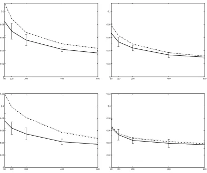
Figure 5: Experimental results on the WebKB corpus, using SVMs for linear (dotted) and Gaussian (dash-dotted) kernels, compared with the diffusion kernel for the multinomial (solid). Classification error for the task of labeling course vs. either faculty, project, or student is shown in these plots, as a function of training set size. The left plot uses tf representation and the right plot uses tfidf representation. The curves shown are the error rates averaged over 20-fold cross validation, with error bars representing one standard deviation. The results for the other “1 vs. all” labeling tasks are qualitatively similar, and are therefore not shown.

40 80 120 200 400 600 0

0.01 0.02 0.03 0.04 0.05 0.06 0.07 0.08

40 80 120 200 400 600 0

0.01 0.02 0.03 0.04 0.05 0.06 0.07 0.08

80 120 200 400 600 0

0.02 0.04 0.06 0.08 0.1

80 120 200 400 600 0

0.02 0.04 0.06 0.08 0.1

80 120 200 400 600 0

0.02 0.04 0.06 0.08 0.1 0.12

80 120 200 400 600 0

0.02 0.04 0.06 0.08 0.1 0.12

40 80 120 200 400 0

0.01 0.02 0.03 0.04 0.05 0.06 0.07

40 80 120 200 400 0

0.01 0.02 0.03 0.04 0.05 0.06 0.07

40 80 120 200 400 0

0.01 0.02 0.03 0.04 0.05 0.06 0.07 0.08 0.09

40 80 120 200 400 0

0.01 0.02 0.03 0.04 0.05 0.06 0.07 0.08 0.09

tf Representation tfidf Representation

Task L Linear Gaussian Diffusion Linear Gaussian Diffusion 40 0.1225 0.1196 0.0646 0.0761 0.0726 0.0514

80 0.0809 0.0805 0.0469 0.0569 0.0564 0.0357

course vs. all 120 0.0675 0.0670 0.0383 0.0473 0.0469 0.0291

200 0.0539 0.0532 0.0315 0.0385 0.0380 0.0238

400 0.0412 0.0406 0.0241 0.0304 0.0300 0.0182

600 0.0362 0.0355 0.0213 0.0267 0.0265 0.0162

40 0.2336 0.2303 0.1859 0.2493 0.2469 0.1947

80 0.1947 0.1928 0.1558 0.2048 0.2043 0.1562

faculty vs. all 120 0.1836 0.1823 0.1440 0.1921 0.1913 0.1420

200 0.1641 0.1634 0.1258 0.1748 0.1742 0.1269

400 0.1438 0.1428 0.1061 0.1508 0.1503 0.1054

600 0.1308 0.1297 0.0931 0.1372 0.1364 0.0933

40 0.1827 0.1793 0.1306 0.1831 0.1805 0.1333

80 0.1426 0.1416 0.0978 0.1378 0.1367 0.0982

project vs. all 120 0.1213 0.1209 0.0834 0.1169 0.1163 0.0834

200 0.1053 0.1043 0.0709 0.1007 0.0999 0.0706

400 0.0785 0.0766 0.0537 0.0802 0.0790 0.0574

600 0.0702 0.0680 0.0449 0.0719 0.0708 0.0504

40 0.2417 0.2411 0.1834 0.2100 0.2086 0.1740

80 0.1900 0.1899 0.1454 0.1681 0.1672 0.1358

student vs. all 120 0.1696 0.1693 0.1291 0.1531 0.1523 0.1204

200 0.1539 0.1539 0.1134 0.1349 0.1344 0.1043

400 0.1310 0.1308 0.0935 0.1147 0.1144 0.0874

600 0.1173 0.1169 0.0818 0.1063 0.1059 0.0802

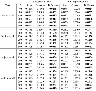
Table 1: Experimental results on the WebKB corpus, using SVMs for linear, Gaussian, and multi-nomial diffusion kernels. The left columns use tf representation and the right columns use tfidf representation. The error rates shown are averages obtained using 20-fold cross validation. The best performance for each training set size L is shown in boldface. All differences are statistically significant according to the paired t test at the 0.05 level.

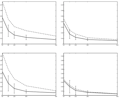
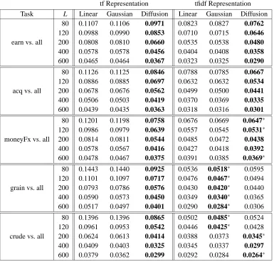
Figure 7 shows the test set error rates for two of the one-versus-all experiments on the Reuters data, where the designated classes were chosen to be acq and moneyFx. All of the results for Reuters one-versus-all tasks are shown in Table 3.

Figure 6 and Figure 8 show representative results for the second type of classification task, where the goal is to discriminate between two specific classes. In the case of the WebKB data the results are shown for course vs. student. In the case of the Reuters data the results are shown for moneyFx vs. earn and grain vs. earn. Again, the results for the other classes are qualitatively similar; the numerical results are summarized in Tables 2 and 4.

tf Representation tfidf Representation

Task L Linear Gaussian Diffusion Linear Gaussian Diffusion 40 0.0808 0.0802 0.0391 0.0580 0.0572 0.0363

80 0.0505 0.0504 0.0266 0.0409 0.0406 0.0251

course vs. student 120 0.0419 0.0409 0.0231 0.0361 0.0359 0.0225

200 0.0333 0.0328 0.0184 0.0310 0.0308 0.0201

400 0.0263 0.0259 0.0135 0.0234 0.0232 0.0159

600 0.0228 0.0221 0.0117 0.0207 0.0202 0.0141

40 0.2106 0.2102 0.1624 0.2053 0.2026 0.1663

80 0.1766 0.1764 0.1357 0.1729 0.1718 0.1335

faculty vs. student 120 0.1624 0.1618 0.1198 0.1578 0.1573 0.1187

200 0.1405 0.1405 0.0992 0.1420 0.1418 0.1026

400 0.1160 0.1158 0.0759 0.1166 0.1165 0.0781

600 0.1050 0.1046 0.0656 0.1050 0.1048 0.0692

40 0.1434 0.1430 0.0908 0.1304 0.1279 0.0863

80 0.1139 0.1133 0.0725 0.0982 0.0970 0.0634

project vs. student 120 0.0958 0.0957 0.0613 0.0870 0.0866 0.0559

200 0.0781 0.0775 0.0514 0.0729 0.0722 0.0472

400 0.0590 0.0579 0.0405 0.0629 0.0622 0.0397

600 0.0515 0.0500 0.0325 0.0551 0.0539 0.0358

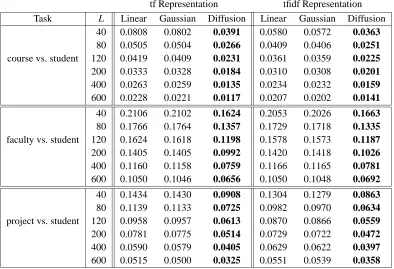
Table 2: Experimental results on the WebKB corpus, using SVMs for linear, Gaussian, and multi-nomial diffusion kernels. The left columns use tf representation and the right columns use tfidf representation. The error rates shown are averages obtained using 20-fold cross validation. The best performance for each training set size L is shown in boldface. All differences are statistically significant according to the paired t test at the 0.05 level.

use L1normalization to give a valid embedding into the probability simplex, while for the linear and

Gaussian kernels we use L2normalization, which works better empirically than L1for these kernels.

The curves show the test set error rates averaged over 20 iterations of cross validation as a function of the training set size. The error bars represent one standard deviation. For both the Gaussian and diffusion kernels, we test scale parameters (√2σfor the Gaussian kernel and 2t1/2for the diffusion kernel) in the set_{0.5,1,2,3,4,5,7,10_}. The results reported are for the best parameter value in that range.

We also performed experiments with the popular Mod-Apte train and test split for the top 10 categories of the Reuters collection. For this split, the training set has about 7000 documents and is highly biased towards negative documents. We report in Table 5 the test set accuracies for the tf representation. For the tfidf representation, the difference between the different kernels is not statistically significant for this amount of training and test data. The provided train set is more than enough to achieve outstanding performance with all kernels used, and the absence of cross validation data makes the results too noisy for interpretation.

tf Representation tfidf Representation

Task L Linear Gaussian Diffusion Linear Gaussian Diffusion 80 0.1107 0.1106 0.0971 0.0823 0.0827 0.0762

120 0.0988 0.0990 0.0853 0.0710 0.0715 0.0646

earn vs. all 200 0.0808 0.0810 0.0660 0.0535 0.0538 0.0480

400 0.0578 0.0578 0.0456 0.0404 0.0408 0.0358

600 0.0465 0.0464 0.0367 0.0323 0.0325 0.0290

80 0.1126 0.1125 0.0846 0.0788 0.0785 0.0667

120 0.0886 0.0885 0.0697 0.0632 0.0632 0.0534

acq vs. all 200 0.0678 0.0676 0.0562 0.0499 0.0500 0.0441

400 0.0506 0.0503 0.0419 0.0370 0.0369 0.0335

600 0.0439 0.0435 0.0363 0.0318 0.0316 0.0301

80 0.1201 0.1198 0.0758 0.0676 0.0669 0.0647∗

120 0.0986 0.0979 0.0639 0.0557 0.0545 0.0531∗

moneyFx vs. all 200 0.0814 0.0811 0.0544 0.0485 0.0472 0.0438

400 0.0578 0.0567 0.0416 0.0427 0.0418 0.0392

600 0.0478 0.0467 0.0375 0.0391 0.0385 0.0369∗

80 0.1443 0.1440 0.0925 0.0536 0.0518∗ 0.0595 120 0.1101 0.1097 0.0717 0.0476 0.0467∗ 0.0494 grain vs. all 200 0.0793 0.0786 0.0576 0.0430 0.0420∗ 0.0440 400 0.0590 0.0573 0.0450 0.0349 0.0340∗ 0.0365 600 0.0517 0.0497 0.0401 0.0290 0.0284∗ 0.0306

80 0.1396 0.1396 0.0865 0.0502 0.0485∗ 0.0524 120 0.0961 0.0953 0.0542 0.0446 0.0425∗ 0.0428 crude vs. all 200 0.0624 0.0613 0.0414 0.0388 0.0373 0.0345∗

400 0.0409 0.0403 0.0325 0.0345 0.0337 0.0297

600 0.0379 0.0362 0.0299 0.0292 0.0284 0.0264∗

Table 3: Experimental results on the Reuters corpus, using SVMs for linear, Gaussian, and multi-nomial diffusion kernels. The left columns use tf representation and the right columns use tfidf representation. The error rates shown are averages obtained using 20-fold cross vali-dation. The best performance for each training set size L is shown in boldface. An asterisk (*) indicates that the difference is not statistically significant according to the paired t test at the 0.05 level.

results of Zhang and Oles (2001), with a+indicating the diffusion kernel F1 measure is greater than the result published in Zhang and Oles (2001) for this task.

tf Representation tfidf Representation

Task L Linear Gaussian Diffusion Linear Gaussian Diffusion 40 0.1043 0.1043 0.1021∗ 0.0829 0.0831 0.0814∗

80 0.0902 0.0902 0.0856∗ 0.0764 0.0767 0.0730∗

acq vs. earn 120 0.0795 0.0796 0.0715 0.0626 0.0628 0.0562

200 0.0599 0.0599 0.0497 0.0509 0.0511 0.0431

400 0.0417 0.0417 0.0340 0.0336 0.0337 0.0294

40 0.0759 0.0758 0.0474 0.0451 0.0451 0.0372∗

80 0.0442 0.0443 0.0238 0.0246 0.0246 0.0177

moneyFx vs. earn 120 0.0313 0.0311 0.0160 0.0179 0.0179 0.0120

200 0.0244 0.0237 0.0118 0.0113 0.0113 0.0080

400 0.0144 0.0142 0.0079 0.0080 0.0079 0.0062

40 0.0969 0.0970 0.0543 0.0365 0.0366 0.0336∗

80 0.0593 0.0594 0.0275 0.0231 0.0231 0.0201∗

grain vs. earn 120 0.0379 0.0377 0.0158 0.0147 0.0147 0.0114∗

200 0.0221 0.0219 0.0091 0.0082 0.0081 0.0069∗

400 0.0107 0.0105 0.0060 0.0037 0.0037 0.0037∗

40 0.1108 0.1107 0.0950 0.0583∗ 0.0586 0.0590 80 0.0759 0.0757 0.0552 0.0376 0.0377 0.0366∗

crude vs. earn 120 0.0608 0.0607 0.0415 0.0276 0.0276∗ 0.0284 200 0.0410 0.0411 0.0267 0.0218∗ 0.0218 0.0225 400 0.0261 0.0257 0.0194 0.0176 0.0171∗ 0.0181

Table 4: Experimental results on the Reuters corpus, using SVMs for linear, Gaussian, and multi-nomial diffusion kernels. The left columns use tf representation and the right columns use tfidf representation. The error rates shown are averages obtained using 20-fold cross vali-dation. The best performance for each training set size L is shown in boldface. An asterisk (*) indicates that the difference is not statistically significant according to the paired t test at the 0.05 level.

The Reuters data is a much larger collection than WebKB, and the document frequency statistics, which are the basis for the inverse document frequency weighting in the tfidf representation, are evidently much more effective on this collection. It is notable, however, that the multinomial in-formation diffusion kernel achieves at least as high an accuracy without the use of any heuristic term weighting scheme. These results offer evidence that the use of multinomial geometry is both theoretically motivated and practically effective for document classification.

6. Discussion and Conclusion

Category Linear RBF Diffusion

earn 0.01159 0.01159 0.01026

acq 0.01854 0.01854 0.01788

money-fx 0.02418 0.02451 0.02219

grain 0.01391 0.01391 0.01060

crude 0.01755 0.01656 0.01490

trade 0.01722 0.01656 0.01689 interest 0.01854 0.01854 0.01689

ship 0.01324 0.01324 0.01225

wheat 0.00894 0.00794 0.00629

corn 0.00794 0.00794 0.00563

Table 5: Test set error rates for the Reuters top 10 classes using tf features. The train and test sets were created using the Mod-Apte split.

Category Linear RBF Diffusion _±

earn 0.9781 0.9781 0.9808 ₋

acq 0.9626 0.9626 0.9660 + money-fx 0.8254 0.8245 0.8320 + grain 0.8836 0.8844 0.9048 ₋

crude 0.8615 0.8763 0.8889 + trade 0.7706 0.7797 0.8050 + interest 0.8263 0.8263 0.8221 + ship 0.8306 0.8404 0.8827 + wheat 0.8613 0.8613 0.8844 ₋

corn 0.8727 0.8727 0.9310 +

Table 6: F1 measure for the Reuters top 10 classes using tf features. The train and test sets were created using the Mod-Apte split. The last column compares the presented results with the published results of Zhang and Oles (2001), with a+indicating the diffusion kernel F1 measure is greater than the result published in Zhang and Oles (2001) for this task.

deal of geometric information about the manifold. While the geometric perspective in statistics has most often led to reformulations of results that can be viewed more traditionally, the kernel methods developed here clearly depend crucially on the geometry of statistical families.