Bias-Variance Analysis of Support Vector Machines for the
Development of SVM-Based Ensemble Methods
Giorgio Valentini [email protected]
DSI - Dipartimento di Scienze dell’Informazione Universit`a degli Studi di Milano
Via Comelico 39, Milano, Italy
Thomas G. Dietterich [email protected]
Department of Computer Science Oregon State University
Corvallis, OR 97331, USA
Editor: Nello Cristianini
Abstract
Bias-variance analysis provides a tool to study learning algorithms and can be used to properly design ensemble methods well tuned to the properties of a specific base learner. Indeed the effec-tiveness of ensemble methods critically depends on accuracy, diversity and learning characteristics of base learners. We present an extended experimental analysis of bias-variance decomposition of the error in Support Vector Machines (SVMs), considering Gaussian, polynomial and dot prod-uct kernels. A characterization of the error decomposition is provided, by means of the analysis of the relationships between bias, variance, kernel type and its parameters, offering insights into the way SVMs learn. The results show that the expected trade-off between bias and variance is sometimes observed, but more complex relationships can be detected, especially in Gaussian and polynomial kernels. We show that the bias-variance decomposition offers a rationale to develop en-semble methods using SVMs as base learners, and we outline two directions for developing SVM ensembles, exploiting the SVM bias characteristics and the bias-variance dependence on the kernel parameters.
Keywords: Bias-variance analysis, support vector machines, ensemble methods, multi-classifier
systems.
1. Introduction
Ensembles of classifiers represent one of the main research directions in machine learning (Diet-terich, 2000a). Empirical studies showed that both in classification and regression problems en-sembles are often much more accurate than the individual base learner that make them up (Bauer and Kohavi, 1999; Dietterich, 2000b; Freund and Schapire, 1996), and recently different theoreti-cal explanations have been proposed to justify the effectiveness of some commonly used ensemble methods (Kittler et al., 1998; Schapire, 1999; Kleinberg, 2000; Allwein et al., 2000).
bias-variance decomposition of the error (Geman et al., 1992), and it shows that ensembles can reduce variance (Breiman, 1996b) and also bias (Kong and Dietterich, 1995).
Recently Domingos proved that Schapire’s notion of margins (Schapire et al., 1998) can be expressed in terms of bias and variance and vice versa (Domingos, 2000c), and hence Schapire’s bounds of ensemble’s generalization error can be equivalently expressed in terms of the distribution of the margins or in terms of the bias-variance decomposition of the error, showing the equivalence of margin-based and bias-variance-based approaches.
The effectiveness of ensemble methods depends on the specific characteristics of the base learn-ers; in particular on the relationship between diversity and accuracy of the base learners (Dietterich, 2000a; Kuncheva et al., 2001b; Kuncheva and Whitaker, 2003), on their stability (Breiman, 1996b; Bousquet and Elisseeff, 2002), and on their general geometrical properties (Cohen and Intrator, 2001).
From this standpoint the analysis of the features and properties of the base learners used in en-semble methods is crucial in order to design enen-semble methods well tuned to the characteristics of a specific base learner. For instance, considering that the agglomeration of many classifiers into one classification rule reduces variance (Breiman, 1996a), we could apply low-bias base learners to reduce both bias and variance using ensemble methods. To this purpose in this paper we study Support Vector Machines (SVMs), that are “strong” dichotomic classifiers, well founded on Vap-nik’s statistical learning theory (Vapnik, 1998), in order to establish if and how we can exploit their specific features in the context of ensemble methods. We analyze the learning properties of SVMs using the bias-variance decomposition of the error as a tool to understand the relationships between kernels, kernel parameters, and learning processes in SVM.
Historically, the bias-variance insight was borrowed from the field of regression, using squared-loss as the squared-loss function (Geman et al., 1992). For classification problems, where the 0/1 loss is the main criterion, several authors proposed bias-variance decompositions related to 0/1 loss. Kong and Dietterich (1995) proposed a bias-variance decomposition in the context of ECOC ensembles (Diet-terich and Bakiri, 1995), but their analysis is extensible to arbitrary classifiers, even if they defined variance simply as a difference between loss and bias.
In Breiman’s decomposition (Breiman, 1996b) bias and variance are always non-negative (while Dietterich definition allows a negative variance), but at any input the reducible error (i.e. the total error rate less noise) is assigned entirely to variance if the classification is unbiased, and to bias if biased. Moreover he forced the decomposition to be purely additive, while for the 0/1 loss this is not the case. Kohavi and Wolpert (1996) approach leads to a biased estimation of bias and variance, assigning a non-zero bias to a Bayes classifier, while Tibshirani (1996) did not use directly the notion of variance, decomposing the 0/1 loss in bias and an unrelated quantity he called “aggregation effect”, which is similar to the James’ notion of variance effect (James, 2003).
Friedman (1997) showed that bias and variance are not purely additive: in some cases increas-ing variance increases the error, but in other cases can also reduce the error, especially when the prediction is biased.
As briefly outlined, these decompositions suffer of significant shortcomings: in particular they lose the relationship to the original squared loss decomposition, forcing in most cases bias and variance to be purely additive.
We consider classification problems and the 0/1 loss function in the Domingos’ unified frame-work of bias-variance decomposition of the error (Domingos, 2000c,b). In this approach bias and variance are defined for an arbitrary loss function, showing that the resulting decomposition spe-cializes to the standard one for squared loss, but it holds also for the 0/1 loss (Domingos, 2000c).
A similar approach has been proposed by James (2003): he extended the notion of variance and bias for general loss functions, distinguishing also between bias and variance, interpreted respec-tively as the systematic error and the variability of an estimator, and the actual effect of bias and variance on the error.
Using Domingos’ theoretical framework, we tried to answer two main questions:
1. Can we characterize bias and variance in SVMs with respect to the kernel and its parameters?
2. Can the bias-variance decomposition offer guidance for developing ensemble methods using SVMs as base learners?
In order to answer these two questions, we planned and performed an extensive series of experiments on synthetic and real data sets to evaluate bias variance-decomposition of the error with different kernels and different kernel parameters.
The paper is organized as follows. In Section 2, we summarize the main results of Domingos’ unified bias-variance decomposition of error. Section 3 outlines how to measure in practice bias and variance decomposition of the error with artificial or large benchmark data sets, or when only a small “real” data set is available. Section 4 outlines the main characteristics of the data sets employed in our experiments and the main experimental tasks performed. Then we present the main results of our experiments about bias-variance decomposition of the error in SVMs, considering separately Gaussian, polynomial and and dot product SVMs, and comparing also the results between different kernels. Section 6 provides a characterization of bias-variance decomposition of the error for Gaussian, polynomial and and dot product SVMs, highlighting the common patterns for each different kernel. Section 7 exploits the knowledge achieved by the bias-variance decomposition of the error to formulate hypotheses about the effectiveness of SVMs as base learners in ensembles of learning machines, and two directions for developing new ensemble models of SVM are proposed. An outline of ongoing and future developments of this work concludes the paper.
2. Bias-Variance Decomposition for the 0/1 Loss Function
The analysis of bias-variance decomposition of the error has been originally developed in the stan-dard regression setting, where the squared error is usually used as loss function. Considering a prediction y= f(x) of an unknown target t, provided by a learner f on input x, with x∈Rd and y∈R, the classical decomposition of the error in bias and variance for the squared error loss is
(Ge-man et al., 1992)
In words, the expected loss of using y to predict t is the sum of the variances of t (noise) and y plus the squared bias. Ey[·]indicates the expected value with respect to the distribution of the random variable y.
This decomposition cannot be automatically extended to the standard classification setting, as in this context the 0/1 loss function is usually applied, and bias and variance are not purely additive. As we are mainly interested in analyzing bias-variance for classification problems, we introduce the variance decomposition for the 0/1 loss function, according to the Domingos unified bias-variance decomposition of the error (Domingos, 2000b).
2.1 Expected Loss Depends on the Randomness of the Training Set and the Target
Consider a (potentially infinite) population U of labeled training data points, where each point is a pair(xj,tj),tj∈
C
,xj ∈Rd,d∈N, whereC
is the set of the class labels. Let P(x,t)be the joint distribution of the data points in U . Let D be a set of m points drawn identically and independently from U according to P. We think of D as being the training sample that we are given for training a classifier. We can view D as a random variable, and we will let ED[·]indicate the expected value with respect to the distribution of D.Let
L
be a learning algorithm, and define fD=L
(D)as the classifier produced byL
applied to a training set D. The model produces a prediction fD(x) =y. Let L(t,y)be the 0/1 loss function, that is L(t,y) =0 if y=t, and L(t,y) =1 otherwise.Suppose we consider a fixed point x∈Rd. This point may appear in many labeled training points in the population. We can view the corresponding labels as being distributed according to the conditional distribution P(t|x). Recall that it is always possible to factor the joint distribution as
P(x,t) =P(x)P(t|x). Let Et[·]indicate the expectation with respect to t drawn according to P(t|x). Suppose we consider a fixed predicted class y for a given x. This prediction will have an expected loss of Et[L(t,y)]. In general, however, the prediction y is not fixed. Instead, it is computed from a model fDwhich is in turn computed from a training sample D.
Hence, the expected loss EL of learning algorithm
L
at point x can be written by considering both the randomness due to the choice of the training set D and the randomness in t due to the choice of a particular test point(x,t):EL(
L
,x) =ED[Et[L(t,fD(x))]],where fD=
L
(D)is the classifier learned byL
on training data D. The purpose of the bias-variance analysis is to decompose this expected loss into terms that separate the bias and the variance.2.2 Optimal and Main Prediction
To derive this decomposition, we must define two things: the optimal prediction and the main
prediction: according to Domingos, bias and variance can be defined in terms of these quantities.
The optimal prediction y∗for point x minimizes Et[L(t,y)]:
y∗(x) =arg min
y Et[L(t,y)]. (1)
makes the optimal prediction at each point x, and corresponds to the Bayes classifier; its error rate corresponds to the Bayes error rate.
The noise N(x), is defined in terms of the optimal prediction, and represents the remaining loss that cannot be eliminated, even by the optimal prediction:
N(x) =Et[L(t,y∗)].
Note that in the deterministic case y∗=t and N(x) =0.
The main prediction ymat point x is defined as
ym=arg min
y0 ED[L(fD(x),y
0)]. (2)
This is a value that would give the lowest expected loss if it were the “true label” of x. It expresses the “central tendency” of a learner, that is its systematic prediction, or, in other words, it is the label for x that the learning algorithm “wishes” were correct. For 0/1 loss, the main prediction is the class predicted most often by the learning algorithm
L
when applied to training sets D.2.3 Bias, Unbiased and Biased Variance.
Given these definitions, the bias B(x)(of a learning algorithm
L
on training sets of size m) is the loss of the main prediction relative to the optimal prediction:B(x) =L(y∗,ym).
For 0/1 loss, the bias is always 0 or 1. We will say that
L
is biased at point x, if B(x) =1. The variance V(x)is the average loss of the predictions relative to the main prediction:V(x) =ED[L(ym,fD(x))]. (3)
It captures the extent to which the various predictions fD(x)vary depending on D.
In the case of the 0/1 loss we can also distinguish two opposite effects of variance (and noise) on the error: in the unbiased case variance and noise increase the error, while in the biased case variance and noise decrease the error.
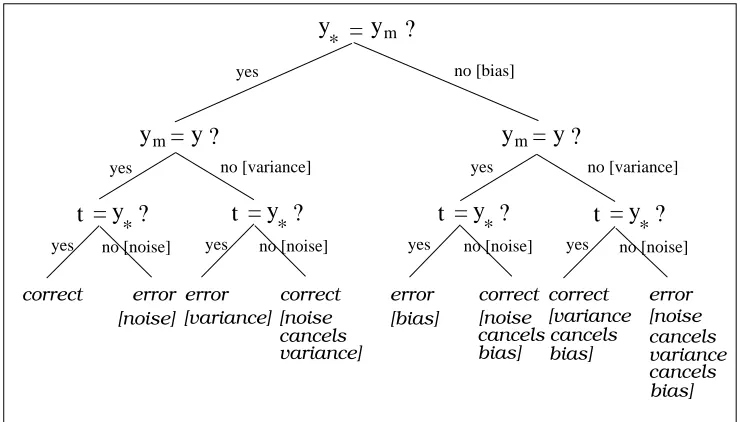
There are three components that determine whether t=y:
1. Noise: is t =y∗?
2. Bias: is y∗=ym? 3. Variance: is ym=y ?
Note that bias is either 0 or 1 because neither y∗nor ymare random variables. From this standpoint we can consider two different cases: the unbiased and the biased case.
In the unbiased case, B(x) =0 and hence y∗=ym. In this case we suffer a loss if the prediction y differs from the main prediction ym(variance) and the optimal prediction y∗is equal to the target t, or y is equal to ym, but y∗is different from t (noise).
In the biased case, B(x) =1 and hence y∗6=ym. In this case we suffer a loss if the prediction y is equal to the main prediction ymand the optimal prediction y∗is equal to the target t, or if both y
y
m*
y
y
m= y ?
y
m= y ?
*
y
=
t
?
*
y
=
t
?
*
y
=
t
?
*
y
=
t
?
=
?
no [variance] no [variance]
no [bias] yes
yes yes
correct
error error correct correct error [noise] [variance] [noise [bias] [noise [variance [noise
variance] bias]cancelsbias] cancels bias] cancels yes yes no [noise] yes no [noise] yes no [noise]
error no [noise] correct
variance cancels
cancels
Figure 1: Case analysis of error.
conditions under which an error can arise, considering the combined effect of bias, variance and noise on the learner prediction.
Considering the above case analysis of the error, if we let P(t6=y∗) =N(x) =τ and P(ym6= y) =V(x) =σ, in the unbiased case we have
L(t,y) = τ(1−σ) +σ(1−τ) (4)
= τ+σ−2τσ
= N(x) +V(x)−2N(x)V(x),
while in the biased case
L(t,y) = τσ+ (1−τ)(1−σ) (5)
= 1−(τ+σ−2τσ)
= B(x)−(N(x) +V(x)−2N(x)V(x)).
Note that in the unbiased case (Equation 4) the variance is an additive term of the loss function, while in the biased case (Equation 5) the variance is a subtractive term of the loss function. Moreover the interaction terms will usually be small, because, for instance, if both noise and variance term will be both lower than 0.1, the interaction term 2N(x)V(x)will be reduced to less than 0.02.
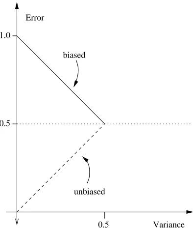
In order to distinguish between these two different effects of the variance on the loss function, Domingos defines the unbiased variance, Vu(x), to be the variance when B(x) =0 and the biased variance, Vb(x), to be the variance when B(x) =1. We can also define the net variance Vn(x)to take into account the combined effect of the unbiased and biased variance:
0.5 1.0
0.5
Variance Error
biased
unbiased
Figure 2: Effects of biased and unbiased variance on the error. The unbiased variance increments, while the biased variance decrements the error.
Figure 2 summarizes in graphic form the opposite effects of biased and unbiased variance on the error.
If we can disregard the noise, the unbiased variance captures the extents to which the learner deviates from the correct prediction ym (in the unbiased case ym=y∗), while the biased variance
captures the extents to which the learner deviates from the incorrect prediction ym (in the biased case ym6=y∗).
2.4 Domingos’ Bias-Variance Decomposition
Domingos (2000a) showed that for a quite general loss function the expected loss is
EL(
L
,x) =c1N(x) +B(x) +c2V(x). (6) For the 0/1 loss function c1 is 2PD(fD(x) =y∗)−1 and c2is +1 if B(x) =0 and−1 if B(x) =1. Note that c2V(x) =Vu(x)−Vb(x) =Vn(x)(Equation 3), and if we disregard the noise, Equation 6 can be simplified toEL(
L
,x) =B(x) +Vn(x). (7)This decomposition for a single point x can be generalized to the entire population by defining
Ex[·]to be the expectation with respect to P(x). Then we can define the average bias Ex[B(x)], the
average unbiased variance Ex[Vu(x)], and the average biased variance Ex[Vb(x)]. In the noise-free case, the expected loss over the entire population is
Ex[EL(
L
,x)] =Ex[B(x)] +Ex[Vu(x)]−Ex[Vb(x)].3. Measuring Bias and Variance
The procedures to measure bias and variance depend on the characteristics and on the cardinality of the data sets used.
For synthetic data sets we can generate different sets of training data for each learner to be trained. Then a large synthetic test set can be generated in order to estimate the bias-variance decomposition of the error for a specific learner model.
Similarly, if a large data set is available, we can split it in a large learning set and in a large testing set. Then we can randomly draw subsets of data from the large training set in order to train the learners; bias-variance decomposition of the error is measured on the large independent test set. However, in practice, for real data we dispose of only one and often small data set. In this case, we can use cross-validation techniques for estimating bias-variance decomposition, but we propose to use out-of-bag (Breiman, 2001) estimation procedures, as they are computationally less expensive.
3.1 Measuring with Artificial or Large Benchmark Data Sets
Consider a set
D
={Di}ni=1 of learning sets Di={xk,tk}mk=1. The data sets Di can be generated according to some known probability distribution or can be drawn with replacement from a large data setD
according to an uniform probability distribution. Here we consider only a two-class case, i.e. tk∈C
={−1,1}, xk∈X, for instance X=Rd, d∈N, but the extension to the multiclass case is straightforward.The estimates of the error, bias, unbiased and biased variance are performed on a test set
T
separated from the training setD. In particular these estimates with respect to a single example
(x,t)∈T
are performed using the classifiers fDi =L
(Di)produced by a learnerL
using training sets Didrawn fromD
. These classifiers produce a prediction y∈C
, that is fDi(x) =y. The estimates are performed for all the(x,t)∈T
, and the overall loss, bias and variance can be evaluated averaging over the entire test setT
.In presence of noise and with the 0/1 loss, the optimal prediction y∗is equal to the label t that is
observed more often in the universe U of data points:
y∗(x) =arg max t∈C P(t|x).
The noise N(x)for the 0/1 loss can be estimated if we can evaluate the probability of the targets for a given example x:
N(x) =
∑
t∈CL(t,y∗)P(t|x) =
∑
t∈C||t6=y∗||P(t|x),
where||z||=1 if z is true, 0 otherwise. In practice it is difficult to estimate the noise for “real world” data sets, and to simplify the computation we consider the noise free case. In this situation we have
The main prediction is a function of the y=fDi(x). Considering a 0/1 loss, we have
ym=arg max(p1,p−1),
where p1=PD(y=1|x)and p−1=PD(y=−1|x), i.e. the main prediction is the mode. To calculate p1, having a test set
T
={xj,tj}rj=1, it is sufficient to count the number of learners that predict class 1 on a given input x:p1(xj) =∑ n
i=1kfDi(xj) =1k
n ,
wherekzk=1 if z is true andkzk=0 if z is false
The bias can be easily calculated after the evaluation of the main prediction:
B(x) =
1 if ym6=t 0 if ym=t
=
ym−t 2 , (8) or equivalently:
B(x) =
1 if pcorr(x)≤0.5 0 otherwise,
where pcorris the probability that a prediction is correct, i.e. pcorr(x) =P(y=t|x) =PD(fD(x) =t). In order to measure the variance V(x), if we define yDi =fDi(x), we have
V(x) =1
n n
∑
i=1
L(ym,yDi) = 1
n n
∑
i=1
||(ym6=yDi)||
The unbiased variance Vu(x)and the biased variance Vb(x)can be calculated evaluating if the prediction of each learner differs from the main prediction respectively in the unbiased and in the biased case:
Vu(x) = 1
n n
∑
i=1
||(ym=t)and(ym6=yDi)||,
Vb(x) = 1
n n
∑
i=1
||(ym6=t)and(ym6=yDi)||.
In the noise-free case, the average loss on the example x ED(x) is calculated by a simple algebraic sum of bias, unbiased and biased variance:
ED(x) =B(x) +Vu(x)−Vb(x) =B(x) + (1−2B(x))V(x).
We can easily calculate the average bias, variance, unbiased, biased and net variance, averaging over the entire set of the examples of the test set
T
={(xj,tj)}rj=1. In the remaining part of this section the indices j refer to the examples that belong to the test setT
, while the indices i refer to the training sets Di, drawn with replacement from the separated training setD, and used to train the
classifiers fDi.The average quantities are
Average bias:
Ex[B(x)] = 1
r r
∑
j=1
B(xj) = 1
r r
∑
j=1
Average variance:
Ex[V(x)] = 1
r r
∑
j=1
V(xj)
= 1
nr r
∑
j=1 n
∑
i=1
L(ym(xj),fDi(xj))
= 1
nr r
∑
j=1 n
∑
i=1
||ym(xj)6=fDi(xj)||,
Average unbiased variance:
Ex[Vu(x)] = 1
r r
∑
j=1
Vu(xj) = 1
nr r
∑
j=1 n
∑
i=1
||(ym(xj) =tj)and(ym(xj)6= fDi(xj))||,
Average biased variance:
Ex[Vb(x)] = 1
r r
∑
j=1
Vb(xj) = 1
nr r
∑
j=1 n
∑
i=1
||(ym(xj)6=tj)and(ym(xj)6= fDi(xj))||,
and the Average net variance:
Ex[Vn(x)] = 1
r r
∑
j=1
Vn(xj) = 1
r r
∑
j=1
(Vu(xj)−Vb(xj)).
Finally, the average loss on all the examples (with no noise) is the algebraic sum of the average bias, unbiased and biased variance.
Ex[L(t,y)] =Ex[B(x)] +Ex[Vu(x)]−Ex[Vb(x)]
3.2 Measuring with Small Data Sets
In practice (unlike in theory), we have only one and often small data set
S
. We can simulate mul-tiple training sets by bootstrap replicates Sb={x|x is drawn at random with replacement fromS
}. In order to measure bias and variance we can use out-of-bag points, providing in such a way an unbiased estimate of the error. At first we need to construct B bootstrap replicates ofS
(e. g.,B=200): S1, . . . ,SB. Then we apply a learning algorithm
L
to each replicate Sbto obtain hypothe-ses fb=L
(Sb).Let Tb=
S
\Sbbe the data points that do not appear in Sb(out of bag points). We can use these data sets Tbto evaluate the bias-variance decomposition of the error; that is we compute the predicted values fb(x),∀x s.t.x∈Tb. For each data point x, we have now the observed corresponding value t and several predictions y1, . . . ,yK, where K=|{Tb|x∈Tb,1≤b≤B}|, K≤B, and on the average K'B/3, because about 1/3 of the predictors is not trained on a specific input x. Note that the value of K depends on the specific example x considered. Moreover if x∈Tb then x∈/Sb, hence fb(x) makes a prediction on an unknown example x.In order to compute the main prediction, for a two-class classification problem, we can define
p1(x) = 1
K B
∑
b=1
p−1(x) = 1
K B
∑
b=1
||(x∈Tb)and(fb(x) =−1)||.
The main prediction ym(x)corresponds to the mode:
ym=arg max(p1,p−1).
The bias can be calculated as in Equation 8, and the variance V(x)is
V(x) = 1
K B
∑
b=1
||(x∈Tb)and(ym6=fb(x))||.
Similarly easily computed are the unbiased, biased and net-variance:
Vu(x) = 1
K B
∑
b=1
||(x∈Tb)and(B(x) =0)and(ym6= fb(x))||,
Vb(x) = 1
K B
∑
b=1
||(x∈Tb)and(B(x) =1)and(ym6= fb(x))||,
Vn(x) =Vu(x)−Vb(x).
Average bias, variance, unbiased, biased and net variance, can be easily calculated averaging over all the examples.
4. Bias-Variance Analysis in SVMs
The bias-variance decomposition of the error represents a powerful tool to analyze learning pro-cesses in learning machines. According to the procedures described in the previous section, we measured bias and variance in SVMs, in order to study the relationships with different kernel types and their parameters. To accomplish this task we computed bias-variance decomposition of the error on different synthetic and “real” data sets.
4.1 Experimental Setup
In the experiments we employed seven different data sets, both synthetic and “real”. P2 is a syn-thetic bidimensional two-class data set;1 each region is delimited by one or more of four simple polynomial and trigonometric functions (Figure 3). The synthetic data set Waveform is generated from a combination of two of three “base” waves; we reduced the original three classes of
Wave-form to two, deleting all samples pertaining to class 0. The other data sets are all from the UCI
repository (Merz and Murphy, 1998). Table 4.1 summarizes the main features of the data sets used in the experiments.
1. The application gensimple, that we developed to generate the data, is freely available on line at
I
II
I I II
I
II
II
0 2 4 6 8 10
0 2 4 6 8 10
X1 X2
Figure 3: P2 data set, a bidimensional two class synthetic data set. Roman numbers label the re-gions belonging to the two classes.
Data set # of # of tr. # of tr. # base # of attr. samples sets tr. set test samples
P2 2 100 400 synthetic 10000
Waveform 21 100 200 synthetic 10000
Grey-Landsat 36 100 200 4425 2000
Letter 16 100 200 614 613
Letter w. noise 16 100 200 614 613
Spam 57 100 200 2301 2300
Musk 166 100 200 3299 3299
Table 1: Data sets used in the experiments.
In order to perform a reliable evaluation of bias and variance we used small training set and large test sets. For synthetic data we generated the desired number of samples. For real data sets we used bootstrapping to replicate the data. In both cases we computed the main prediction, bias, unbiased and biased variance, net-variance according to the procedures explained in Section 3.1. In our experiments, the computation of James’ variance and systematic effect (James, 2003) is reduced to the measurements of the net-variance and bias, and hence we did not explicitly compute these quantities (see Appendix A for details).
Waveform. The test sets were chosen reasonably large (10000 examples) to obtain reliable estimates
of bias and variance.
For real data sets we first divided the data into a training
D
and a testT
sets. If the data sets had a predefined training and test sets reasonably large, we used them (as in Grey-Landsat and Spam), otherwise we split them in a training and test set of equal size. Then we drew fromD
bootstrap samples. We chose bootstrap samples much smaller than|T
|(100 examples). More precisely we drew 200 data sets fromD
, each one consisting of 100 examples uniformly drawn with replacement. Summarizing, both with synthetic and real data sets we generated small training sets for each data set and a much larger test set. Then all the data were normalized in such a way that for each attribute the mean was 0 and the standard deviation 1. In all our experiments we usedNEUROb-jects (Valentini and Masulli, 2002),2 a C++ library for the development of neural networks and machine learning applications, and SVM-light (Joachims, 1999), a set of C applications for training and testing SVMs.
We developed and used the C++ applicationanalyze BV, to perform bias-variance decompo-sition of the error.3 This application analyzes the output of a generic learning machine model and computes the main prediction, error, bias, net-variance, unbiased and biased variance using the 0/1 loss function. Other C++ applications have been developed to process and analyze the results, using also Cshell scripts to train, test and analyze bias-variance decomposition of all the SVM models for each specific data set.
4.2 Experimental Tasks
To evaluate bias and variance in SVMs we conducted experiments with different kernels (Gaussian, polynomial and dot product) and different kernel parameters. For each kernel we considered the same set of values for the parameter C that controls the trade-off between training error and margin, ranging from C=0.01 to C=1000.
1. Gaussian kernels. We evaluated bias-variance decomposition varying the parametersσ of the kernel and the C parameter. In particular we analyzed:
(a) The relationships between average error, bias, net-variance, unbiased and biased vari-ance, theσparameter of the kernel and the C parameter.
(b) The relationships between generalization error, training error, number of support vectors and capacity with respect toσ.
We trained RBF-SVM with all the combinations of the parametersσand C, using the a set of values forσranging fromσ=0.01 toσ=1000. We evaluated about 200 different RBF-SVM models for each data set.
2. Polynomial kernels. We evaluated bias-variance decomposition varying the degree of the kernel and the C parameter. In particular we analyzed the relationships between average error, bias, net-variance, unbiased and biased variance, the degree of the kernel and the C parameter.
2. This library may be downloaded from the web athttp://www.disi.unige.it/person/ValentiniG/NEURObjects. 3. The source code is available atftp://ftp.disi.unige.it/person/ValentiniG/BV. Moreover C++ classes for
0.02 0.1 0.2 0.5 1 2 5 10 20 50 100 sigma 0.01 1 5 20 100 1000 C 0 0.1 0.2 0.3 0.4 0.5 Avg. err. 0.01 (a) 0.02 0.1 0.2 0.5 1 2 5 10 20 50 100 sigma 0.01 1 5 20 100 1000 C 0 0.1 0.2 0.3 0.4 0.5 Bias 0.01 0.02 0.1 0.2 0.5 1 2 5 10 20 50 100 sigma 0.01 1 5 20 100 1000 C -0.1 0 0.1 0.2 0.3 0.4 Net var. 0.01 (b) (c) 0.02 0.1 0.2 0.5 1 2 5 10 20 50 100 sigma 0.01 1 5 20 100 1000 C 0 0.1 0.2 0.3 0.4 0.5 Unb. var.
0.01 0.10.02
0.2 0.5 1 2 5 10 20 50 100 sigma 0.01 1 5 20 100 1000 C 0 0.1 0.2 0.3 0.4 0.5 Biased var. 0.01 (d) (e)
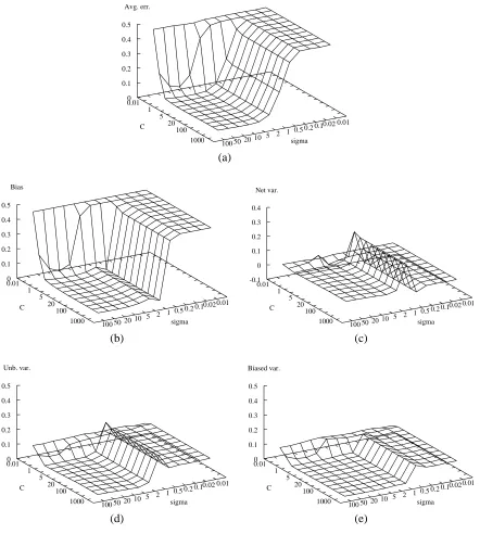
Figure 4: Grey-Landsat data set. Error (a) and its decomposition in bias (b), net variance (c), unbi-ased variance (d), and biunbi-ased variance (e) in SVM RBF, varying both C andσ.
about 120 different polynomial-SVM models for each data set. Following the heuristic of Jakkola, the dot product of polynomial kernel was divided by the dimension of the input data, to “normalize” the dot product before to raise to the degree of the polynomial.
3. Dot product kernels. We evaluated bias-variance decomposition varying the C parameter. We analyzed the relationships between average error, bias, net-variance, unbiased and biased variance and the parameter C (the regularization factor) of the kernel. We trained dot-product-SVM considering different values for the C parameter, evaluating in such a way 12 different dot-product-SVM models for each data set.
Each SVM model required the training of 200 different SVMs, one for each synthesized or boot-strapped data set, for a total of (204+120+12)×200=67200 trained SVM for each data set (134400 for the data set P2, as for this data set we used 400 data sets for each model). The ex-periments required the training of more than half million of SVMs, considering all the data sets and of course the testing of all the SVM previously trained in order to evaluate the bias-variance decomposition of the error of the different SVM models. For each SVM model we computed the main prediction, bias, net-variance, biased and unbiased variance and the error on each example of the test set, and the corresponding average quantities on the overall test set.
5. Results
In this section we present the results of the experiments. We analyzed bias-variance decomposition with respect to the kernel parameters considering separately Gaussian, polynomial and dot product SVMs, comparing also the results among different kernels. Here we present the main results. Full
results, data and graphics are available by anonymous ftp atftp://ftp.disi.unige.it/person/ValentiniG/papers/bv-svm.ps.gz.
5.1 Gaussian Kernels
Figure 4 depicts the average loss, bias net-variance, unbiased and biased variance varying the values ofσand the regularization parameter C in RBF-SVM on the Grey-Landsat data set. We note thatσ is the most important parameter: although for very low values of C the SVM cannot learn, indepen-dently of the values ofσ, (Figure 4 a), the error, the bias, and the net-variance depend mostly on theσparameter. In particular for low values ofσ, bias is very high (Figure 4 b) and net-variance is 0, as biased and unbiased variance are about equal (Figure 4d and 4e). Then the bias suddenly drops (Figure 4b), lowering the average loss (Figure 4a), and then stabilizes for higher values of
σ. Interestingly enough, in this data set (but also in others, data not shown), we note an increment followed by a decrement of the net-variance, resulting in a sort of “wave shape” of the net variance graph (Figure 4c).
Bias and average loss increases with σonly for very small C values. Note that net-variance and bias show opposite trends only for small values of C (Figure 5 c). For larger C values the symmetric trend is limited only to σ≤1 (Figure 5 d), otherwise bias stabilizes and net-variance slowly decreases. Figure 6 shows more in detail the effect of the C parameter on bias-variance decomposition. For C≥1 there are no variations of the average error, bias and variance for a fixed value ofσ. Note that for very low values ofσ(Figure 6a and b) there is no learning. In the Letter-Two data set, as in other data sets (figures not shown), only for small C values we have variations in bias and variance values (Figure 6).
5.1.1 DISCRIMINANTFUNCTIONCOMPUTED BY THESVM-RBF CLASSIFIER
In order to get insights into the behaviour of the SVM learning algorithm with Gaussian kernels we plotted the real-valued functions computed without considering the discretization step performed through the sign function. The real valued function computed by a Gaussian SVM is
f(x,α,b) =
∑
i∈SVyiαiexp(−kxi−xk2/σ2) +b,
where theαiare the Lagrange multipliers found by the solution of the dual optimization problem, the xi∈SV are the support vectors, that is the points for whichαi>0.
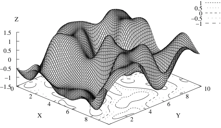
We plotted the surface computed by the Gaussian SVM with the synthetic data set P2. Indeed it is the only surface that can be easily visualized, as the data are bidimensional and the resulting real valued function can be easily represented through a wireframe three-dimensional surface. The SVMs are trained with exactly the same training set composed by 100 examples. The outputs are referred to a test set of 10000 examples, selected in an uniform way through all the data domain. In particular we considered a grid of equi-spaced data at 0.1 interval in a two dimensional 10×10 input space. If f(x,α,b)>0 then the SVM matches up the example x with class 1, otherwise with class 2.
With small values of σ we have “spiky” functions: the response is high around the support vectors, and is close to 0 in all the other regions of the input domain (Figure 7). In this case we have overfitting: a large error on the test set (about 46 % withσ=0.01 and 42.5 % withσ=0.02 ), and a training error near to 0.
If we enlarge the values of σwe obtain a wider response on the input domain and the error decreases (withσ=0.1 the error is about 37 %). With σ=1 we have a smooth function that fits quite well the data (Figure 8). In this case the error drops down to about 13 %.
Enlarging too muchσwe have a too smooth function (Figure 9 (a)), and the error increases to about 37 %: in this case the high bias is due to an excessive smoothing of the function. Increasing the values of the regularization parameter C (in order to better fit the data), we can diminish the error to about 15 %: the shape of the function now is less smooth (Figure 9 (b)).
5.1.2 BEHAVIOR OFSVMS WITHLARGEσVALUES
Fig 4 and 5 show that σparameter plays a sort of smoothing effect, as the value of σincreases. In particular with large values of σ we did not observe any increment of bias nor decrement of variance. In order to get insights into this counter-intuitive behaviour we tried to answer these two questions:
1. Does the bias increase while variance decrease with large values ofσ, and what is the com-bined effect of bias-variance on the error?
2. In this situation (large values forσ), what is the effect of the C parameter?
In Figure 5 we do not observe an increment of bias with large values ofσ, but we limited our experiments to values ofσ≤100. Here we investigate the effect for larger values ofσ(from 100 to 1000).
In most cases, also increasing the values ofσright to 1000 we do not observe an increment of the bias and a substantial decrement of the variance. Only for low values of C, that is C<1, the bias and the error increase with large values ofσ(Figure 10). With the P2 data set the situation is different: in this case we observe an increment of the bias and the error with large values ofσ, even if with large values of C the increment rate is lower (Figure 11 a and b).
Also with the musk data set we note an increment of the error with very large values ofσ, but surprisingly this is due to an increment of the unbiased variance, while the bias is quite stable, at least for values of C>1, (Figure 11 c and d).
Larger values of C counter-balance the bias introduced by large values of σ. But with some distributions of the data too large values ofσproduce too smooth functions, and also incrementing C it is very difficult to fit the data. Indeed, the discriminant function computed by the RBF-SVM with the P2 data set (that is the function computed without considering the sign function) is too smooth for large values ofσ: forσ=20, the error is about 37%, due almost entirely to the large bias, (Figure 9 a), and forσ=500 the error is about 45 % and also incrementing the C value to 1000, we obtain a surface that fits the data better, but with an error that remains large (about 35%). Indeed with very large values ofσthe Gaussian kernel becomes nearly linear (Scholkopf and Smola, 2002) and if the data set is very far from being linearly separable, as with the P2 data set (Figure 3), the error increases, especially in the bias component (Figure 11 (a) and (b)). Summarizing with large
σvalues bias can increment, while net-variance tends to stabilize, but this effect can be counter-balanced by larger C values.
5.1.3 RELATIONSHIPS BETWEENGENERALIZATIONERROR, TRAININGERROR, NUMBER OF
SUPPORT VECTORS ANDCAPACITY
Looking at Figure 4 and 5, we see that SVMs do not learn for small values ofσ. Moreover the low error region is relatively large with respect toσand C.
In this section we evaluate the relationships between the estimated generalization error, the bias, the training error, the number of support vectors and the estimated Vapnik Chervonenkis dimension, in order to answer the following questions:
1. Why SVMs do not learn for small values ofσ?
3. Can we use the variation of the number of support vectors to predict the “low error” region?
4. Is there any relationship between the bias, variance and VC dimension, and can we use this last one to individuate the “low error” region?
The generalization error, bias, training error, number of support vectors and the Vapnik Cher-vonenkis dimension are estimated averaging with respect to 400 SVMs (P2 data set) or 200 SVMs (other data sets) trained with different bootstrapped training sets composed by 100 examples each one. The test error and the bias are estimated with respect to an independent and sufficiently large data set.
The VC dimension is estimated using the Vapnik’s bound based on the radius R of the sphere that contains all the data (in the feature space), approximated through the sphere centered in the origin, and on the norm of the weights in the feature space (Vapnik, 1998). In this way the VC dimension is overestimated but it is easy to compute and we are interested mainly in the comparison of the VC dimension of different SVM models:
VC≤R2· kwk2+1,
where
kwk2=
∑
i∈SVj∑
∈SVαiαjK(xi,xj)yiyj
and
R2=max
i K(xi,xi).
The number of support vectors is expressed as the halved ratio of the number (% SV ) of support vectors with respect to the total number of training data:
%SV= #SV
#trainingdata·2.
In the graphs shown in Figure 12 and Figure 13, on the left y axis is represented the error, training error and bias, and the halved ratio of support vectors. On the right y axis is reported the estimated Vapnik Chervonenkis dimension.
For very small values ofσthe training error is very small (about 0), while the number of support vectors is very high, and high is also the error and the bias (Figure12 and 13). These facts support the hypothesis of overfitting problems with small values of σ. Indeed the real-valued function computed by the SVM (that is the function computed without considering the sign function, see Section 5.1.1) is very spiky with small values ofσ(Figure 7). The response of the SVM is high only in small areas around the support vectors, while in all the other areas “not covered” by the support vectors the response is very low (about 0), that is the SVM is not able to get a decision, with a consequently very high bias. In the same region (small values for σ) the net variance is usually very small, for either one of these reasons: 1) biased and unbiased variance are almost equal because the SVM performs a sort of random guessing for the most part of the unknown data; 2) both biased and unbiased variance are about 0, showing that all the SVMs tend to answer in the same way independently of a particular instance of the training set (Figure 5 a, b and f). Enlarging
SVM can decide also on unknown examples. At the same time the number of support vectors decreases (Figure 12 and 13).
Considering the variation of the ratio of the support vectors withσ, in all data sets the trend of the rate of support vectors follows the error, with a sigmoid shape that sometimes becomes an U shape for small values of C (Figure12 and 13). This is not surprising because it is known that the support vector ratio offers an approximation of the generalization error of the SVMs (Vapnik, 1998). Moreover, on all the data sets the %SV decreases in the “stabilized” region, while in the transition region remains high. As a consequence the decrement in the number of support vectors shows that we are entering the “low error” region, and in principle we can use this information to detect this region.
In our experiments, an inspection of the support vectors relative to the Grey-Landsat and
Wave-form data sets found that most of the support vectors are shared in polynomial and Gaussian kernels
with respectively the best degree andσparameters. Even if these results confirmed the ones found by other authors (see e.g. Vapnik (1998)), it is worth noting that we did not perform a system-atic study on this topic: we considered only two data sets and we compared only few hundreds of different SVMs.
In order to analyze the role of the VC dimension on the generalization ability of learning ma-chines, we know from statistical learning theory that the form of the bounds of the generalization error E of SVMs is
E(f(σ,C)k
n))≤Eemp(f(σ,C)kn)) +Φ( hk
n ), (9)
where f(σ,C)k
nrepresents the set of functions computed by an RBF-SVM trained with n examples and with parameters(σk,Ck)taken from a set of parameters S={(σi,Ci),i∈N}, Eemp represents the empirical error andΦthe confidence interval that depends on the cardinality n of the data set and on the VC dimension hk of the set of functions identified by the actual selection of the parameters (σk,Ck). In order to obtain good generalization capabilities we need to minimize both the empirical risk and the confidence interval. According to Vapnik’s bounds (Equation 9), in Figure 12 and 13 the lowest generalization error is obtained for a small empirical risk and a small estimated VC dimension.
But sometimes with relatively small values of VC we may have a very large error, as the training error and the number of support vectors increase with very large values ofσ(Figure 12 a and 13 a). Moreover with a very large estimate of the VC dimension and low empirical error (Figure 12 and 13) we may have a relatively low generalization error. In conclusion it seems very difficult to use in practice these estimate of the VC dimension to infer the generalization abilities of the SVM. In particular it seems unreliable to use the VC dimension to infer the “low error” region of the RBF-SVM.
5.2 Polynomial and Dot Product Kernels
In this section we analyze the characteristics of bias-variance decomposition of the error in polyno-mial SVMs, varying the degree of the kernel and the regularization parameter C.
Average error and bias tends to be higher for low C and degree values, but, incrementing the degree, the error is less sensitive to C values (Figure 16).
Bias is flat (Figure 17 a) or decreasing with respect to the degree (Figure 15 b), or it can be con-stant or decreasing, depending on C (Figure 17 b). Unbiased variance shows an U shape (Figure 14 a and b) or it increases (Figure 14 c) with respect to the degree, and the net-variance follows the shape of the unbiased variance. Note that in the P2 data set (Figure 15) bias and net-variance follow the classical opposite trends with respect to the degree. This is not the case with other data sets (see, e.g. Figure 14).
For large values of C bias and net-variance tend to converge, as a result of the bias reduction and net-variance increment (Figure 18), or because both stabilize at similar values (Figure 16).
In dot product SVMs bias and variance show opposite trends: bias decreases, while net-variance and unbiased net-variance tend to increase with C (Figure 19). On the data set P2 this trend is not observed, as in this task the bias is very high and the SVM does not perform better than random guessing (Figure 19a). The minimum of the average loss for relatively low values of C is the result of the decrement of the bias and the increment of the net-variance: it is achieved usually before the crossover of bias and net-variance curves and before the stabilization of the bias and the net-variance for large values of C. The biased variance remains small independently of C.
5.3 Comparing Kernels
In this section we compare the bias-variance decomposition of the error with respect to the C pa-rameter, considering Gaussian, polynomial and dot product kernels. For each kernel and for each data set the best results are selected. Table 5.3 shows the best results achieved by the SVM, con-sidering each kernel and each data set used in the experiments. Interestingly enough in 3 data sets (Waveform, Letter-Two with added noise and Spam) there are not significant differences in the error between the kernels, but there are differences in bias, net-variance, unbiased or biased variance. In the other data sets Gaussian kernels outperform polynomial and dot product kernels, lowering bias or net-variance or both. Considering bias and net-variance, in some cases they are lower for poly-nomial or dot product kernel, showing that different kernels learn in different ways with different data.
Considering the data set P2 (Figure 20 a, c, e), RBF-SVMs achieve the best results, as bias is lower. Unbiased variance is comparable between polynomial and Gaussian kernel, while net-variance is lower, as biased net-variance is higher for polynomial-SVM. In this task the bias of dot product SVM is very high. Also in the data set Musk (Figure 20 b, d, f) RBF-SVM obtains the best results, but in this case unbiased variance is responsible for this fact, while bias is similar. With the other data sets the bias is similar between RBF-SVM and polynomial-SVM, but for dot product SVM often the bias is higher (Figure 21 b, d, f). Interestingly enough RBF-SVM seems to be more sensible to the C value with respect to both polynomial and dot product SVM: for
Parameters Avg. Bias Var. Var. Net
Error unb. bias. Var.
Data set P2
RBF-SVM C=20, σ=2 0.1516 0.0500 0.1221 0.0205 0.1016 Poly-SVM C=10, degree=5 0.2108 0.1309 0.1261 0.0461 0.0799 D-prod SVM C=500 0.4711 0.4504 0.1317 0.1109 0.0207 Data set Waveform
RBF-SVM C=1, σ=50 0.0706 0.0508 0.0356 0.0157 0.0198 Poly-SVM C=1, degree=1 0.0760 0.0509 0.0417 0.0165 0.0251 D-prod SVM C=0.1 0.0746 0.0512 0.0397 0.0163 0.0234 Data set Grey-Landsat
RBF-SVM C=2, σ=20 0.0382 0.0315 0.0137 0.0069 0.0068 Poly-SVM C=0.1,degree=5 0.0402 0.0355 0.0116 0.0069 0.0047 D-prod SVM C=0.1 0.0450 0.0415 0.0113 0.0078 0.0035 Data set Letter-Two
RBF-SVM C=5, σ=20 0.0743 0.0359 0.0483 0.0098 0.0384 Poly-SVM C=2, degree=2 0.0745 0.0391 0.0465 0.0111 0.0353 D-prod SVM C=0.1 0.0908 0.0767 0.0347 0.0205 0.0142 Data set Letter-Two with added noise
RBF-SVM C=10, σ=100 0.3362 0.2799 0.0988 0.0425 0.0563 Poly-SVM C=1, degree=2 0.3432 0.2799 0.1094 0.0461 0.0633 D-prod SVM C=0.1 0.3410 0.3109 0.0828 0.0527 0.0301 Data set Spam
RBF-SVM C=5, σ=100 0.1263 0.0987 0.0488 0.0213 0.0275 Poly-SVM C=2, degree=2 0.1292 0.0969 0.0510 0.0188 0.0323 D-prod SVM C=0.1 0.1306 0.0965 0.0547 0.0205 0.0341 Data set Musk
RBF-SVM C=2, σ=100 0.0884 0.0800 0.0217 0.0133 0.0084 Poly-SVM C=2, degree=2 0.1163 0.0785 0.0553 0.0175 0.0378 D-prod SVM C=0.01 0.1229 0.1118 0.0264 0.0154 0.0110
-0.1 0 0.1 0.2 0.3 0.4 0.5
0.01 0.02 0.1 0.2 0.5 1 2 5 10 20 50 100 sigma avg. error bias net variance unbiased var. biased var C=10 -0.1 0 0.1 0.2 0.3 0.4 0.5
0.01 0.02 0.1 0.2 0.5 1 2 5 10 20 50 100 sigma avg. error bias net variance unbiased var. biased var C=10 (a) (b) -0.1 0 0.1 0.2 0.3 0.4 0.5
0.01 0.02 0.1 0.2 0.5 1 2 5 10 20 50 100 avg. error bias net variance unbiased var. biased var C=0.1 sigma -0.1 0 0.1 0.2 0.3 0.4 0.5
0.01 0.02 0.1 0.2 0.5 1 2 5 10 20 50 100 sigma avg. error bias net variance unbiased var. biased var C=1 (c) (d) -0.1 0 0.1 0.2 0.3 0.4 0.5
0.01 0.02 0.1 0.2 0.5 1 2 5 10 20 50 100 sigma avg. error bias net variance unbiased var. biased var C=10 -0.1 0 0.1 0.2 0.3 0.4 0.5
0.01 0.02 0.1 0.2 0.5 1 2 5 10 20 50 100 sigma avg. error bias net variance unbiased var. biased var C=1 (e) (f)
-0.1 0 0.1 0.2 0.3 0.4 0.5
0.01 0.1 1 2 5 10 20 50 100 200 500 1000 C avg. error bias net variance unbiased var. biased var σ=0.01 -0.1 0 0.1 0.2 0.3 0.4 0.5
0.01 0.1 1 2 5 10 20 50 100 200 500 1000 C avg. error bias net variance unbiased var. biased var σ=0.1 (a) (b) -0.1 0 0.1 0.2 0.3 0.4 0.5
0.01 0.1 1 2 5 10 20 50 100 200 500 1000 C avg. error bias net variance unbiased var. biased var σ=1 -0.1 0 0.1 0.2 0.3 0.4 0.5
0.01 0.1 1 2 5 10 20 50 100 200 500 1000 C avg. error bias net variance unbiased var. biased var σ=5 (c) (d) -0.1 0 0.1 0.2 0.3 0.4 0.5
0.01 0.1 1 2 5 10 20 50 100 200 500 1000 C avg. error bias net variance unbiased var. biased var σ=20 -0.1 0 0.1 0.2 0.3 0.4 0.5
0.01 0.1 1 2 5 10 20 50 100 200 500 1000 C avg. error bias net variance unbiased var. biased var σ=100 (e) (f)
0.5 0 −0.5 −1
0 2
4 6
8 X
2 4
6 8
10
Y −1.5
−1 −0.5 0 0.5 1
Z
Figure 7: The real valued function computed by the SVM on the P2 data set withσ=0.01, C=1.
1 0.5 0 −0.5 −1
0 2
4 6
8 X
2 4
6 8
10
Y −1.5
−1 −0.5 0 0.5 1 1.5
Z
1 0 −1 0 2 4 6 8 X 2 4 6 8 10 Y −2 −1.5 −1 −0.5 0 0.5 1 1.5 Z 10 0 −10 0 2 4 6 8 X 2 4 6 8 10 Y −20 −15 −10 −5 0 5 10 15 20 Z (a) (b) 1 0.5 0 −0.5 −1 0 2 4 6 8 X 2 4 6 8 10 Y −1.5 −1 −0.5 0 0.5 1 1.5 Z 1 0 −1 −2 0 2 4 6 8 X 2 4 6 8 10 Y −3 −2.5−2 −1.5−1 −0.50 0.51 1.52 Z (c) (d)
Figure 9: The real valued function computed by the SVM on the P2 data set. (a)σ=20 C=1, (b)
0 0.1 0.2 0.3 0.4 0.5
0.01 0.02 0.1 0.2 0.5 1 2 5 10 20 50 100 200 300 400 500 1000 avg. error
bias net variance unbiased var. biased var
sigma C=0.1
0 0.1 0.2 0.3 0.4 0.5
0.01 0.02 0.1 0.2 0.5 1 2 5 10 20 50 100 200 300 400 500 1000 sigma
avg. error bias net variance unbiased var. biased var C=1
(a) (b)
0 0.1 0.2 0.3 0.4 0.5
0.01 0.02 0.1 0.2 0.5 1 2 5 10 20 50 100 200 300 400 500 1000 sigma
avg. error bias net variance unbiased var. biased var C=10
0 0.1 0.2 0.3 0.4 0.5
0.01 0.02 0.1 0.2 0.5 1 2 5 10 20 50 100 200 300 400 500 1000 sigma
avg. error bias net variance unbiased var. biased var C=100
(c) (d)
0 0.1 0.2 0.3 0.4 0.5
0.01 0.02 0.1 0.2 0.5 1 2 5 10 20 50 100 200 300 400 500 1000 sigma
avg. error bias net variance unbiased var. biased var C=1
0 0.1 0.2 0.3 0.4 0.5
0.01 0.02 0.1 0.2 0.5 1 2 5 10 20 50 100 200 300 400 500 1000 sigma
avg. error bias net variance unbiased var. biased var C=1000
(a) (b)
0 0.05 0.1 0.15 0.2
0.01 0.02 0.1 0.2 0.5 1 2 5 10 20 50 100 200 300 400 500 1000 sigma
avg. error bias net variance unbiased var. biased var C=1
0 0.05 0.1 0.15 0.2
0.01 0.02 0.1 0.2 0.5 1 2 5 10 20 50 100 200 300 400 500 1000 sigma
avg. error bias net variance unbiased var. biased var C=1000
(c) (d)
VC dim. Error 0 0.1 0.2 0.3 0.4 0.5
0.01 0.02 0.1 0.2 0.5 1 2 5 10 20 50 100 200 300 400 500 1000 0 225 450 675 900 sigma C=1 gen. error bias train error %SV VC dim. VC dim. Error 0 0.1 0.2 0.3 0.4 0.5
0.01 0.02 0.1 0.2 0.5 1 2 5 10 20 50 100 200 300 400 500 1000 0 225 450 675 900 sigma C=10 gen. error bias train error %SV VC dim. (a) (b) VC dim. Error 0 0.1 0.2 0.3 0.4 0.5
0.01 0.02 0.1 0.2 0.5 1 2 5 10 20 50 100 200 300 400 500 1000 0 225 450 675 900 sigma C=100 gen. error bias train error %SV VC dim. VC dim. Error 0 0.1 0.2 0.3 0.4 0.5
0.01 0.02 0.1 0.2 0.5 1 2 5 10 20 50 100 200 300 400 500 1000 0 225 450 675 900 sigma C=1000 gen. error bias train error %SV VC dim. (c) (d)
VC dim. Error 0 0.1 0.2 0.3 0.4 0.5
0.01 0.02 0.1 0.2 0.5 1 2 5 10 20 50 100 200 300 400 500 1000 0 100 200 300 400 sigma C=1 gen. error bias train error %SV VC dim. VC dim. Error 0 0.1 0.2 0.3 0.4 0.5
0.01 0.02 0.1 0.2 0.5 1 2 5 10 20 50 100 200 300 400 500 1000 0 100 200 300 400 sigma C=10 gen. error bias train error %SV VC dim. (a) (b) VC dim. Error 0 0.1 0.2 0.3 0.4 0.5
0.01 0.02 0.1 0.2 0.5 1 2 5 10 20 50 100 200 300 400 500 1000 0 100 200 300 400 sigma C=100 gen. error bias train error %SV VC dim. VC dim. Error 0 0.1 0.2 0.3 0.4 0.5
0.01 0.02 0.1 0.2 0.5 1 2 5 10 20 50 100 200 300 400 500 1000 0 100 200 300 400 sigma C=1000 gen. error bias train error %SV VC dim. (c) (d)
0 0.02 0.04 0.06 0.08 0.1 0.12
1 2 3 4 5 6 7 8 9 10 polynomial degree
avg. error bias net variance unbiased var. biased var C=0.1
0 0.02 0.04 0.06 0.08 0.1 0.12
1 2 3 4 5 6 7 8 9 10 polynomial degree
avg. error bias net variance unbiased var. biased var C=50
(a) (b)
0 0.05 0.1 0.15 0.2
1 2 3 4 5 6 7 8 9 10 polynomial degree
avg. error bias net variance unbiased var. biased var C=0.1
0 0.05 0.1 0.15 0.2
1 2 3 4 5 6 7 8 9 10 polynomial degree
avg. error bias net variance unbiased var. biased var C=50
(c) (d)
Figure 14: Bias-variance decomposition of the error in bias, net variance, unbiased and biased vari-ance in polynomial SVM, while varying the degree and for some fixed values of C: (a) Waveform, C=0.1, (b) Waveform, C=50, (c) Letter-Two, C=0.1, (d) Letter-Two,
2 3 4 5 6 7 8 9 10 degree 0.1 1 2 5 10 20 100 500 C 0 0.05 0.1 0.15 0.2 0.25 0.3 0.35 0.4 Avg. err. (a) 2 3 4 5 6 7 8 9 10 degree 0.1 1 2 5 10 100 500 C 0 0.05 0.1 0.15 0.2 0.25 0.3 0.35 0.4 Bias
20 3 2
4 5 6 7 8 9 10 degree 0.1 1 2 5 10 100 500 C 0 0.05 0.1 0.15 0.2 0.25 0.3 0.35 0.4 Net var. 20 (b) (c)
Figure 15: P2 data set. Error (a) and its decomposition in bias (b) and net variance (c), varying both
-0.1 0 0.1 0.2 0.3 0.4 0.5
0.01 0.1 1 2 5 10 20 50 100 200 500 1000 C
avg. error bias net variance unbiased var. biased var degree=2
-0.1 0 0.1 0.2 0.3 0.4 0.5
0.01 0.1 1 2 5 10 20 50 100 200 500 1000 C
avg. error bias net variance unbiased var. biased var degree=3
(a) (b)
-0.1 0 0.1 0.2 0.3 0.4 0.5
0.01 0.1 1 2 5 10 20 50 100 200 500 1000 C
avg. error bias net variance unbiased var. biased var degree=5
-0.1 0 0.1 0.2 0.3 0.4 0.5
0.01 0.1 1 2 5 10 20 50 100 200 500 1000 C
avg. error bias net variance unbiased var. biased var degree=10
(c) (d)
1 2 3 4 5 6 7 8 9 10 degree 0.01 1 5 20 100 1000 C 0 0.05 0.1 0.15 0.2 Bias 1 2 3 4 5 6 7 8 9 10 degree 0.01 1 5 20 100 1000 C 0 0.1 0.2 0.3 0.4 0.5 Bias (a) (b)
Figure 17: Bias in polynomial SVMs with (a) Waveform and (b) Spam data sets, varying both C and polynomial degree.
0 0.05 0.1 0.15 0.2 0.25 0.3 0.35 0.4
0.01 0.1 1 2 5 10 20 50 100 200 500 1000 C avg. error bias net variance unbiased var. biased var degree=6 -0.1 0 0.1 0.2 0.3 0.4
0.01 0.1 1 2 5 10 20 50 100 200 500 1000 C avg. error bias net variance unbiased var. biased var degree=3 (a) (b)
0 0.1 0.2 0.3 0.4 0.5 0.6
0.01 0.1 1 2 5 10 20 50 100 200 500 1000 C avg. error bias net variance unbiased var. biased var 0 0.01 0.02 0.03 0.04 0.05 0.06 0.07 0.08
0.01 0.1 1 2 5 10 20 50 100 200 500 1000 C avg. error bias net variance unbiased var. biased var (a) (b) 0 0.05 0.1 0.15 0.2
0.01 0.1 1 2 5 10 20 50 100 200 500 1000 C avg. error bias net variance unbiased var. biased var 0 0.1 0.2 0.3 0.4 0.5
0.01 0.1 1 2 5 10 20 50 100 200 500 1000 C avg. error bias net variance unbiased var. biased var (c) (d) 0 0.05 0.1 0.15 0.2 0.25
0.01 0.1 1 2 5 10 20 50 100 200 500 1000 C avg. error bias net variance unbiased var. biased var 0 0.05 0.1 0.15 0.2
0.01 0.1 1 2 5 10 20 50 100 200 500 1000 C avg. error bias net variance unbiased var. biased var (e) (f)
0 0.1 0.2 0.3 0.4 0.5
0.01 0.1 1 2 5 10 20 50 100 200 500 1000 C avg. error bias net variance unbiased var. biased var σ=1 -0.05 0 0.05 0.1 0.15 0.2
0.01 0.1 1 2 5 10 20 50 100 200 500 1000 C avg. error bias net variance unbiased var. biased var σ=100 (a) (b) 0 0.1 0.2 0.3 0.4 0.5
0.01 0.1 1 2 5 10 20 50 100 200 500 1000 C avg. error bias net variance unbiased var. biased var degree=5 -0.05 0 0.05 0.1 0.15 0.2
0.01 0.1 1 2 5 10 20 50 100 200 500 1000 C avg. error bias net variance unbiased var. biased var degree=2 (c) (d) 0 0.1 0.2 0.3 0.4 0.5 0.6
0.01 0.1 1 2 5 10 20 50 100 200 500 1000 C avg. error bias net variance unbiased var. biased var -0.05 0 0.05 0.1 0.15 0.2
0.01 0.1 1 2 5 10 20 50 100 200 500 1000 C avg. error bias net variance unbiased var. biased var (e) (f)
0 0.05 0.1 0.15 0.2
0.01 0.1 1 2 5 10 20 50 100 200 500 1000 C avg. error bias net variance unbiased var. biased var σ=20 0 0.05 0.1 0.15 0.2 0.25 0.3
0.01 0.1 1 2 5 10 20 50 100 200 500 1000 C avg. error bias net variance unbiased var. biased var σ=20 (a) (b) 0 0.05 0.1 0.15 0.2
0.01 0.1 1 2 5 10 20 50 100 200 500 1000 C avg. error bias net variance unbiased var. biased var degree=3 0 0.05 0.1 0.15 0.2 0.25 0.3
0.01 0.1 1 2 5 10 20 50 100 200 500 1000 C avg. error bias net variance unbiased var. biased var degree=2 (c) (d) 0 0.05 0.1 0.15 0.2
0.01 0.1 1 2 5 10 20 50 100 200 500 1000 C avg. error bias net variance unbiased var. biased var 0 0.05 0.1 0.15 0.2 0.25 0.3
0.01 0.1 1 2 5 10 20 50 100 200 500 1000 C avg. error bias net variance unbiased var. biased var (e) (f)
Kernel Avg. Bias Var. Var. Net
type Error unb. bias. Var.
RBF 0.0901±0.0087 0.0805±0.0126 0.0237±0.0039 0.0141±0.0025 0.0096±0.0019 Poly 0.1158±0.0069 0.0782±0.0083 0.0585±0.0071 0.0109±0.0018 0.0376±0.0047 D-prod 0.1305±0.0133 0.1179±0.0140 0.0285±0.0084 0.0159±0.0045 0.0126±0.0035
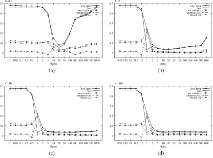
Table 3: Evaluation of the variation of the estimated values of bias variance decomposition with the Musk data set. RBF-SVM stands for SVM with Gaussian kernel; Poly-SVM for SVM with polynomial kernel and D-prod SVM for SVM with dot product kernel. Net Var. Var unb. and Var. bias. stand for net, unbiased and biased variance. For each value is represented the mean value over 100 replicated experiments and the corresponding value of the standard deviation.
In our experiments we used relatively small training sets (100 examples), while the number of input variables ranged from 2 (P2 data set) to 166 (Musk data set). Hence, even if for each SVM model (that is for each combination of SVM parameters) we used 200 training sets Di,1≤ i≤200 in order to train 200 different classifiers fDi, you could wonder whether the estimated quantities (average error, bias, net-variance, unbiased and biased variance) could be noisy. An extensive evaluation of the sensitivity of the estimated quantities to the sampling procedure would be very expensive. Indeed if we replicate only 10 times our experiments on all the data sets, we should train and test more than 5 millions of different SVMs. Anyway, in order to get insights about this problem, we performed 100 replicates of our experiments limited only to the Musk data set (that is the data set with the largest dimensionality in our experiments), for a subset of the parameters near the optimal ones. We found that the standard deviation of the estimated values is not too large. For instance, considering the best model for Gaussian, polynomial and dot product kernels we obtained the values shown in Table 5.3. It seems that the computed quantities are not too noisy, even if we need more experiments to confirm this result.
5.4 Bias-Variance Decomposition with Noisy Data
While the estimation of the noise is quite straightforward with synthetic data, it is a difficult task with “real” data James (2003). For these reasons, and in order to simplify the computation and the overall analysis, in our experiments we did not explicitly consider noise.
Anyway, noise can play a significant role in the bias-variance analysis. Indeed, according to Domingos, with the 0/1 loss the noise is linearly added to the error with a coefficient equal to 2PD(fD(x) =y∗)−1 (Equation 6). Hence, if the classifier is accurate, that is if PD(fD(x) =y∗)0.5,
then the noise N(x), if present, influences the expected loss. In the opposite situation also, with very bad classifiers, that is when PD(fD(x) =y∗)0.5, the noise influences the overall error in the op-posite sense: it reduces the expected loss. If PD(fD(x) =y∗)≈0.5, that is if the classifier performs
a sort of random guessing, then 2PD(fD(x) =y∗)−1≈0 and the noise has no substantial impact on
the error.