Exact Bayesian Structure Discovery in Bayesian Networks

Exact Bayesian Structure Discovery in Bayesian Networks

Mikko Koivisto [email protected]

HIIT Basic Research Unit Department of Computer Science University of Helsinki

FIN-00014 Helsinki, Finland

Kismat Sood [email protected]

National Public Health Institute Department of Molecular Medicine FIN-00251 Helsinki, Finland

Editor: David Maxwell Chickering

Abstract

Learning a Bayesian network structure from data is a well-motivated but computationally hard task. We present an algorithm that computes the exact posterior probability of a subnetwork, e.g., a di-rected edge; a modified version of the algorithm finds one of the most probable network structures. This algorithm runs in time O(n2n+nk+1C(m)), where n is the number of network variables, k is a constant maximum in-degree, and C(m)is the cost of computing a single local marginal condi-tional likelihood for m data instances. This is the first algorithm with less than super-exponential complexity with respect to n. Exact computation allows us to tackle complex cases where existing Monte Carlo methods and local search procedures potentially fail. We show that also in domains with a large number of variables, exact computation is feasible, given suitable a priori restrictions on the structures; combining exact and inexact methods is also possible. We demonstrate the appli-cability of the presented algorithm on four synthetic data sets with 17, 22, 37, and 100 variables. Keywords: complex interactions, dynamic programming, layering, structure learning

1. Introduction

Structure discovery in Bayesian networks has attracted a great deal of research over the last decade. A Bayesian network specifies a joint probability distribution of a set of random variables in a struc-tured fashion. A key component in this model is the network structure, a directed acyclic graph on the variables, encoding a set of conditional independence assertions. Learning unknown depen-dencies from data is motivated by a broad collection of applications in prediction and inference (Heckerman et al., 1995b).

structures grows super-exponentially with respect to the number of network variables, exact com-putations are often found infeasible. Indeed, it is known that finding an optimal Bayesian network structure is NP-hard even when the maximum in-degree is bounded by a constant greater than one (Chickering et al., 1995). Consequently, much of the research has focused on inexact methods.

To find a good or an optimal network structure, various generic heuristics, like stochastic local search and genetic algorithms, have been used (see, e.g., Heckerman et al., 1995a; Larra ˜naga et al., 1996). These methods can be also extended to find equivalence classes of network structures (for recent advances, see Chickering, 2002; Acid and de Campos, 2003; Castelo and Ko ˇcka, 2003). A central problem in all these algorithms is that one cannot guarantee the quality of the output. Also, the time requirement, though often practical, may be difficult to estimate beforehand.

Discovering high-probable structural features has not been studied so extensively. Madigan and York (1995) propose a Markov chain Monte Carlo (MCMC) method in the space of network structures. Friedman and Koller (2003) design a more efficient MCMC procedure in the space of variable orders. These algorithms output approximate posterior probabilities of structural features. The approximation quality is not guaranteed in finite runs.

Exact algorithms for structure learning have been presented for very restricted classes of Bayesian networks only. The algorithm by Cooper and Herskovits (1992) is polynomial in the number of vari-ables, but a consistent ordering of the variables is assumed as an input. Chow and Liu (1968) give an efficient algorithm for learning tree structures (i.e., maximum in-degree is one). However, the most efficient exact algorithms, thus far, that allow for arbitrary network structures have super-exponential time complexity (Cooper and Herskovits, 1992; Friedman and Koller, 2003). Consequently, they can be applied only when the number of variables is very small (say, at most 10). Interestingly, however, Chickering (2002) shows that under certain monotonicity assumptions, a greedy search method will find a so called inclusion optimal network structure when the data size approaches infinity—but the time requirement can be exponential.

In this paper, we propose a novel exact algorithm for structure discovery in Bayesian networks of a moderate size (say, 25 variables or less). In fact, we consider two versions of the algorithm: one for computing posterior probabilities of structural features; another for finding an optimal structure. We also present a rigorous complexity analysis of the algorithm. This work is motivated by three serial observations summarized below.

First, we can expect that existing methods fail in cases where the posterior “landscape” of net-work structures is highly complex, including multiple “modes”. This is the case especially when the underlying dependencies show no marginal signals. That is, the edges cannot be detected based on pairwise correlations (which may be all zero). Then it is necessary to consider all possible local dependency structures. This motivates the efforts to extend the scope of exact computation.

Second, it turns out that there are essentially two parallel contributions to the complexity of exact computation. One is due to consideration of all possible local dependency structures in light of the data. This part is unavoidable and may, in practice, actually dominate the overall complexity. Additively to this, another contribution is due to exploration of all graph structures. Although this seems to take more than polynomial time, it turns out that this part does not depend on the size of the data nor the complexity of local models. Thus, for a sufficiently small number of network variables, we really can afford exact exploration through all network structures.

that averages (or alternatively maximizes) over all network structures in less than super-exponential time.

The remainder of this paper is organized as follows. In Section 2, we recall the ingredients of Bayesian networks and the task of structure discovery. Following the work of Buntine (1991), Cooper and Herskovits (1992), and Friedman and Koller (2003) we, in Section 3, describe the idea of conditioning by orders. Based on this, Section 4 presents a novel algorithm for averaging over all network structures. In Section 5, we modify this algorithm to handle the maximization problem. Possible extensions for large networks are sketched in Section 6. In Section 7, we provide experimental results on four synthetic data sets. Finally, Section 8 concludes with a brief discussion.

2. Preliminaries

We define a Bayesian network as a probability model for a vector x= (x1, . . . ,xn)of random

vari-ables. Throughout this paper, we work on the index set V={1, . . . ,n}rather than on the set of the random variables. If S={i1, . . . ,ir}is a subset of V with i1<· · ·<ir, we let xS denote the vector (xi1, . . . ,xir). A graph structure of a Bayesian network specifies conditional independencies among

the variables. We represent the graph structure as a vector G= (G1, . . . ,Gn), where each Gi is a

subset of V and specifies the parents xGi of xi. Only acyclic graphs are valid, so that given a graph

structure, the probability of x is composed by local conditional distributions p(xi|xGi,θ)as

p(x|G,θ) = n

∏

i=1

p(xi|xGi,θ). (1)

Usually local distributions are of some common parametric form, such as Bernoulli or linear Gaus-sian. Therefore we here include the parameters θexplicitly in the conditional part. A Bayesian network is specified by a graph structure and a collection of associated conditional distributions.

Bayesian networks can be used to model multiple vectors x[1], . . . ,x[m], henceforth called data. Throughout this paper we assume that the data is complete, i.e., there are no missing (unobserved) values. To incorporate the idea of learning from data, the vectors are judged to be exchangeable1 (but not independent) so that the probability of the data, given the graph structure, can be expressed as

p(x[1], . . . ,x[m]|G) =

Z

Θp(θ|G)

m

∏

t=1

p(x[t]|G,θ)dθ. (2)

Here each term p(x[t]|G,θ)decomposes as in (1). Thus, when modeling multiple vectors in this way, a collection of Bayesian networks parametrized byθ∈Θis considered and a prior distribution p(θ|G)is assigned to the parameters. A natural application for (2) is the prediction of future events based on past observations.

Henceforth, we denote all the data briefly by x. Accordingly, for i∈V we let xidenote the vector (xi[1], . . . ,xi[m]).

When the graph structure is not known, it is subject to learning. After introducing a prior on the graph structures, we can write

p(x) =

∑

p(G)p(x|G).

This gives the distribution of data which can be used, e.g., in prediction tasks. Unfortunately, averaging over all graph structures is notoriously hard, as the number of possible graphs is found to be at least 2(n2)_{and thus super-exponential in the number of variables. Also, bounding the in-degree,} i.e., the number of parents, per each variable by a constant k does not help much, a lower bound still being at least 2kn log n(for large enough n).

Sometimes, the interest is in the graph structure as such. Then it is appropriate to consider the posterior distribution of the graph structures, which by Bayes rule is given by

p(G|x) = p(G)p(x|G) p(x) .

Various computational methods have been dedicated to the problem of finding a plausible graph structure. Unfortunately, finding a structure that maximizes the posterior probability,

ˆ

G∈arg max

G

p(G|x),

is known to be NP-hard in general (Chickering et al., 1995). But there are also statistical limits for this approach. Namely, searching for a single structure may not be most relevant, since exponen-tially many graph structures can be almost equally probable in light of modest amount of data.

An alternative approach is to compute local summaries of the posterior distribution of the graph structures. In restricted forms this idea appears already in the works of Buntine (1991) and Cooper and Herskovits (1992) but is significantly further developed by Friedman and Koller (2003). Friedman and Koller consider several types of local structural features, such as edges and Markov-blankets. More precisely, if f is the indicator of a structural feature, we are interested in the posterior

p(f |x) =

∑

p(G|x)f(G).

Here the indicator f is supposed to take value 1 if the feature is present and 0 otherwise. By turning to a clever decomposition of the space of possible graph structures, Friedman and Koller find an efficient MCMC method to estimate the above sum. We next review some key parts of their approach.

3. Conditioning on Orders

There is an efficient way to sum over an exponential number of graph structures that are consistent with a fixed order of variables. The key insight of Friedman and Koller (2003) is to use this result, originally due to Buntine (1991), to average over graph structures: they integrate over possible orders by MCMC. We next review the idea of conditioning on orders; MCMC methods will be only briefly mentioned in Section 6.

We define an order of variables as a total order on the index set V . We represent an order≺as a vector(U1, . . . ,Un), where Uigives the predecessors of i in the order, i.e.,

Ui={j∈V : j≺i}.

We say that a graph structure(G1, . . . ,Gn)is consistent with an order(U1, . . . ,Un), denoted G⊆≺,

set of directed acyclic graphs. Note that for different orders, these subsets overlap. Actually, from this we get a fairly tight upper bound n! 2(n2) _{for the number of acyclic graphs. Asymptotically this} is o((2+ε)(n2))_{for any fixed} ε>_{0, and gives thus a much tighter characterization than the usual} bounds 3(n2) _{or 2}Θ(n2)_{(see, e.g., Friedman and Koller, 2003).}

Friedman and Koller (2003) observe that, from the computational point of view, it is advan-tageous to treat different variable orders as mutually exclusive events. While this is somewhat unnatural, since the corresponding sets of consistent graphs are overlapping, this approach is math-ematically valid. Thus, in what follows, a graph structure alone does not determine whether an order is present or not. Therefore, we augment the prior of graph structures to a joint prior on orders and graphs. We also assume some fairly standard modularity assumptions stated below; related definitions are given, e.g., by Cooper and Herskovits (1992) and Friedman and Koller (2003).

Definition 1 We say that a Bayesian network model p is modular over ≺,G,θ and x, or simply order-modular or modular, if the following properties hold:

(M1) If G is consistent with an order≺, then

p(≺,G) =c n

∏

i=1

qi(Ui)q0i(Gi),

where qi and q0i are probability distributions on the subsets of V− {i}for each i, and c is a normalization constant. Otherwise, if≺is not a total order or if G is not consistent with≺, then p(≺,G) =0.

(M2) Given a structure G, the parametersθdecompose into(θ1,G1, . . . ,θn,Gn)such that

p(θ|G) = n

∏

i=1

p(θi,Gi|Gi),

and p(xi|xGi,θ) =p(xi|xGi,θi,Gi)for all i.

We note that while the above described augmentation is convenient, the semantics of the variable order becomes somewhat strange, thus making the elicitation of the prior distribution potentially dif-ficult. However, one can avoid introducing a joint prior if one agrees with the resulting marginal prior distribution, p(G), on graph structures. In that case the role of orders and associated probabil-ity distributions is technical. It is important to note that, in general, we do not have p(Gi) =q0_i(Gi).

Namely the prior p(Gi)favors sets Githat are small and thus consistent with many orders. Yet, it is

easily seen that we have the following simple transform when conditioning by an order.

Proposition 2 If p is modular and G is a graph structure consistent with an order≺, then

p(G|≺) = n

∏

i=1

p(Gi|Ui),

where p(Gi|Ui) =q0i(Gi)/∑G0i⊆Uiq

We give two examples to elucidate the relationship between orders and graphs. First, let each qi and q0i be uniform. Then it is not difficult to conclude that p(Gi |Ui) =2−|Ui| and that p(≺) =

1/n!. However, we note that, with this choice, the distribution of the number of parents is not uniform. In our second example qi is again uniform, however, we set q0i(Gi) to be proportional to

1/ n_|G−1

i|

for parents Giwith cardinality at most the maximum in-degree. This assignment is natural

when different cardinalities of parents are judged to be uniformly distributed. Note, however, that averaging over orders renders the marginal distribution of the cardinality|Gi|slightly biased from

uniform, since small cardinalities are favored as they are consistent with more orders.

While Proposition 2 above essentially follows from property (M1) of Definition 1, another ap-pealing consequence of modularity is due to property (M2). Namely, the distribution of the data remains factorized when the parametersθare marginalized out. A more precise statement is given below; the proof is simple and standard, and therefore omitted.

Proposition 3 If p is modular, x is complete, and G is a graph structure, then

p(x|G) = n

∏

i=1

p(xi|xGi),

where p(xi|xGi) = R

p(θi,Gi |Gi)p(xi|xGi,θi,Gi)dθi,Gi.

We proceed to consider probabilities of local features. Here we restrict our attention to modular features.

Definition 4 A mapping f from graph structures onto{0,1}is called modular if f(G) =∏n

i=1fi(Gi) where each fiis a mapping from the subsets of V− {i}onto{0,1}.

For example, the indicator of a directed edge between two nodes is clearly modular. Also, the constant functions 1 and 0 are trivially modular. More generally, the indicator of any subgraph (a directed acyclic graph on a subset of V ) is modular.

The key observation is that the summation over graph structures decomposes into a product of “local summations” (Buntine, 1991; Friedman and Koller, 2003).

Theorem 5 If p and f are modular, x is complete, and≺= (U1, . . . ,Un)is a variable order, then p(x,f |≺) =

∏

i∈VG

∑

p(Gi|Ui)p(xi|xGi)fi(Gi).

Proof Using first the marginalization and chain rules of probability, and then Proposition 2,

Propo-sition 3, and Definition 4 to the three terms, respectively, we get

p(x,f|≺) =

∑

p(G|≺)p(x|G,≺)p(f|x,G,≺)

=

∑

G1⊆U1 · · ·

∑

Gn⊆Un

n

∏

i=1

p(Gi|Ui)p(xi|xGi)fi(Gi),

which factorizes into the desired product.

The posterior of the feature is obtained via Bayes rule:

Note that the probability of the data, p(x|≺)can be represented as p(x,f0 |≺)where feature f0 is the constant function 1.

Finally, once having the conditional probabilities for the feature, the unconditional posterior is obtained as

p(f|x) =

∑

p(≺|x)p(f|x,≺). (3)

Here ≺runs through all orders on the set V . There are n! different orders, which is still super-exponential with respect to n. Yet, this is much less than the number of all possible graph structures. Friedman and Koller (2003) propose an MCMC method to estimate sum (3) by drawing a sample of orders from the posterior p(≺|x)∝p(≺)p(x|≺). They argue that this approach is more efficient than MCMC directly in the space of graph structures (Madigan and York, 1995).

It is important to note that, despite of the closed form expression of Theorem 5, the compu-tations, given an order, may be quite expensive. Namely, one has to consider all possible sets of parents for each variable. For a fixed maximum number of parents, k, roughly nk+1terms p(xi|xGi),

henceforth called local conditional marginals, need to be computed. Depending on the data size, on the functional forms of the local conditional distributions, and on the value k, this may con-tribute significantly to the total computational complexity. Henceforth we suppose that any local term p(xi|xGi)can be computed in time O(C(m)), where C is a function of data size. For example,

when a local conditional distributions is taken from the exponential family with appropriate con-jugate priors, then the associated C(m)is linear in m. For more structured models, e.g., decision graphs (Chickering et al., 1997), the complexity of computing local conditional marginals can be significantly greater, yet often linear in m.

4. Summation by Dynamic Programming

We next show how the summation over orders can be carried out in roughly n2noperations, which grows much slower than n!. This improved requirement should be contrasted with the lower bound nk+1 (with a potentially large constant factor). For moderate n (say, n<20) and relatively large k (say, k=5), the total complexity may be dominated by the polynomial term. Yet, the computations are feasible on modern computers.

We consider a summation that is slightly different from (3). We write

p(f |x) =p(f,x)/p(x), (4)

and continue by considering evaluation of

p(f,x) =

∑

p(≺)p(f,x|≺). (5)

Note that p(x)is of the same form.

In order to facilitate the forthcoming development, we define for each i∈V a functionαi as

follows. Let i be an element of V and let S be a subset of V that does not contain i. We define

αi(S) =

∑

Gi⊆S

q0_i(Gi)p(xi|xGi)fi(Gi). (6)

In essence, the function αi gives the contribution of the ith local component (xi and its unknown

(2)

(1, 2) (1 ,3) (2, 1) (2, 3)

(3)

(3, 1) (3, 2)

(2, 3, 1) (3, 2, 1) (1)

(1, 3, 2)

(1, 2, 3) (2, 1, 3) (3, 1, 2) ( )

{1} {3}

{1, 2} {1, 3} {2, 3}

{ }

{2}

{1, 2, 3}

(a) (b)

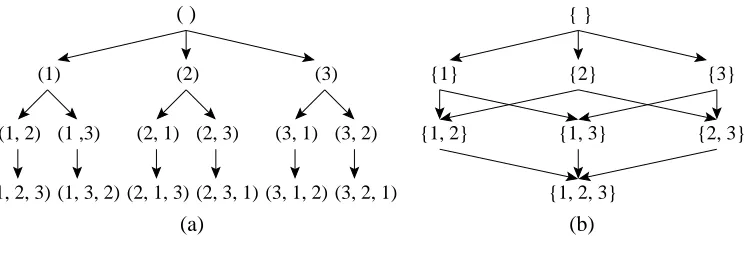
Figure 1: Illustrations of (a) the permutation tree and (b) the subset lattice of{1,2,3}. The nodes of the permutation tree are labeled by the corresponding paths from the root. (The labels of the edges are not shown but can be easily deduced.)

as a way to split the problem of evaluating sum (5) into two steps. The first is to compute these functions given a feature f and a data set x. The second task is to compute sum (5), given the functionsαi. We first consider the latter problem assuming that the functionsαiare precomputed;

we will later come back to the former problem.

It turns out that the sum over orders is advantageous to compute in a manner of variable elim-ination. Here variables refer to the n elementsσ1, . . . ,σn∈V , whereσj is the jth element in the

order. A key observation is that when considering the parents of variable xσj it is sufficient to know

the unordered set{σ1, . . . ,σj−1}of the possible parents. In other words, the order of the possible

parents is irrelevant.

One way to view this reduction from ordered sets to unordered sets is to consider a permutation tree. A permutation tree of V ={1, . . . ,n}is a rooted (directed) tree with n levels. Any node at the hth level has n−h children labeled by distinct elements from V , so that the labels on any (directed) path are all distinct. Thus, a path from the root to a leaf corresponds to a unique permutation on V (see Figure 1(a)). Evaluation of the sum over orders is carried out by a propagation algorithm, where each node obtains a value by summing up the values of its parents, each multiplied by a quantity that depends on the associated path (details will be given soon). However, apart from the last label of the path, only the unordered set of the labels matters. This means that computations over different paths can be merged. Graphically, the permutation tree collapses to a subset lattice. A subset lattice of V is a graph, where nodes corresponds to subsets of V and there is an edge from A to B if and only if B=A∪ {i}for some i6∈A (see Figure 1(b)).

We summarize the above discussion more formally:

Proposition 6 If p and f are modular and x is complete, then

p(f,x) =c g(V),

where c is the normalizing constant and g is defined for all subsets S of V recursively by

g(S) =

∑

with boundary g(/0) =1.

Proof By simple induction we get that

g(V) =

∑

σ1,...,σn

n

∏

j=1

qi(Sj)ασj(Sj),

where(σ1, . . . ,σn)runs through all permutations on V , and Sj={σ1, . . . ,σj−1}. Thus, each(σ1, . . . ,σn)

is a realization of an order≺= (U1, . . . ,Un)withσ1≺σ2≺ · · · ≺σnand Uσj ={σ1, . . . ,σj−1}=Sj.

By the modularity of p, we have

c n

∏

i=1

qi(Ui)q0i(Gi) =p(≺)p(G|≺).

Thus, by (5), Proposition 2, and Theorem 5, we have c g(V) =p(x,f).

This result gives us a relatively efficient way to sum over orders in the manner of dynamic programming (for a related algorithm, see Bellman, 1962). Provided that each value of the functions qi,αi, and g can be accessed in a constant (amortized) time, we have an O(n2n)time algorithm for

computing the posterior p(f |x). Note that the constant c cancels out in (4).

We now take a step back and consider the computation of the functionsαi. Since the

represen-tation of each functionαialready takes 2n−1numbers, the best we can hope is to find an algorithm

that runs in time O(2n). We next show how to achieve this optimal time complexity.2 Consider a fixed i∈V . It is convenient to define a new function,βi, by

βi(Gi) =q0_i(Gi)p(xi|xGi)fi(Gi) for all Gi⊆V− {i}. (8)

Hence, by the definition ofαi we have

αi(S) =

∑

T⊆S

βi(T) for all S⊆V− {i}.

The operator that in this way maps a function of subsets of V−{i}to another such function is known as the M¨obius transform (on the subset lattice of V− {i}). We say thatαi is the M¨obius transform

ofβi.

How fast can we evaluate the M ¨obius transform? In the following discussion we assume that the values ofβi are precomputed and can be accessed in a constant (amortized) time. The

straight-forward approach is to compute separately for each subset S the summation over its subsets. We see that one step takes O(2|S|)time, and hence, the total time complexity is O(3n). To reduce this bound, we notice that βi(T) vanishes for all T with more than k elements. This yields the com-plexity O(nk2n). An alternative, and more efficient approach is to use the fast M ¨obius transform algorithm (see, e.g., Kennes and Smets, 1991). It takes advantage of the overlapping parts of the 2n summations and runs in time O(n2n). However, it does not exploit the in-degree bound k. We next show that under this additional constraint we can still slightly reduce the time complexity, to the desired O(2n).

FAST-TRUNCATED-M ¨OBIUS-TRANSFORM(h0, k)

1 for j←1 to n do

2 for each S⊆N with|S∩ {j+1, . . . ,n}| ≤k do

3 hj(S)←0

4 if|S∩ {j, . . . ,n}| ≤k then 5 hj(S)←hj−1(S)

6 if j∈S then

7 hj(S)←hj(S) +hj−1(S− {j})

8 return hn

Figure 2: An algorithm for evaluating the truncated M ¨obius transform on the subset lattice of N= {1, . . . ,n}. Input h0is the function to be transformed, and k is a number between 1 and n.

We extend the notion of M ¨obius transform by defining a truncated M ¨obius transform as a M¨obius transform where the summation over subsets is restricted to subsets with at most k elements, where k is an additional input parameter. Figure 2 describes a general algorithm for computing trun-cated M¨obius transforms on the subset lattice of N={1, . . . ,n}. (When we apply this algorithm to compute a functionαi, we replace n by n−1.) The algorithm mainly follows the steps of the

stan-dard fast M¨obius transform algorithm (see, e.g., Kennes and Smets, 1991) and splits the transform into n smaller transforms, each being a summation over the two subsets of a singleton {j} ⊆N. These n transforms operate one after another, the jth transform to the result of the(j−1)th trans-form. This procedure can be also viewed as a variable elimination algorithm, where for each{j} “its subset” is treated as a variable taking two values. In the fast truncated M ¨obius transform algo-rithm, described in Figure 2, this standard algorithm is modified so that each of the n transforms is evaluated only at as few subsets of N as needed. While the last transform has to be evaluated at all 2nsubsets, a polynomial number of evaluations is sufficient for the first transforms. Details of this discussion are given in the proof of the following result.

Proposition 7 Algorithm FAST-TRUNCATED-M ¨OBIUS-TRANSFORM(Figure 2) with input(h0,k) runs in time O(2n)for a constant k and computes the function hn, given by

hn(S) =

∑

h0(T) for all S⊆N.

Proof We show by induction on j that hj(S)for S⊆N with|S∩ {j+1, . . . ,n}| ≤k, computed at

the jth iteration, is given by

hj(S) =

∑

· · ·

∑

1(|T1,j∪Sj+1,n| ≤k)h0(T1,j∪Sj+1,n), (9)

where we denote Sr=S∩ {r}and Sr,r0=S_r∪S_r+1∪ · · · ∪S_r0 =S∩ {r,r+1, . . . ,r0}(similarly for T_r and Tr,r0).

In the case j=0 expression (9) trivially holds. We proceed by letting j>0. Let S⊆N with |S∩ {j+1, . . . ,n}| ≤k. We separate two cases, Sj=/0and Sj={j}, and show that expression (9)

First consider the case Sj= /0. By the algorithm, after the jth step, we have

hj(S) =hj−1(S).

Using the induction assumption (9) for hj−1, it is easy to verify that hj(S)can be expressed as in the

induction claim (9) since Tj=Sj=/0.

Then consider the remaining case, Sj={j}. After the jth step, we have

hj(S) =1(|S∩ {j, . . . ,n}| ≤k)hj−1(S) +hj−1(S− {j}).

The first term in the sum corresponds to the case Tj =Sj ={j} in the summation (9). By the

induction assumption (9) for hj−1, it is sufficient to verify that

1(|S∩ {j, . . . ,n}| ≤k)1(|T1,j−1∪Sj,n| ≤k) =1(|T1,j∪Sj+1,n| ≤k),

and that T1,j−1∪Sj,n=T1,j∪Sj+1,n. The latter is obvious since Tj=Sj. The former identity follows

since S∩ {j, . . . ,n}=Sj,n. Note that the condition |S∩ {j, . . . ,n}| ≤k ensures that hj has been

evaluated at S in the previous iteration.

The second term in the sum, hj−1(S− {j}), corresponds to the case Tj= /0. In this case,|T1,j∪ Sj+1,n| ≤k holds since we have assumed that|S∩ {j+1, . . . ,n}| ≤k. The argument of h0remains

invariant because in expression (9) for hj−1(S− {j}), we have Tj=Sj= /0.

We have now shown that (9) holds for all j=1, . . . ,n. Particularly, in the case j=n we get the claimed transformation. This completes the first part of the proof.

We next show that the algorithm runs in time O(2n_{). For the steps j=n−k+1, . . . ,n the}

required total number of operations is proportional to

n

∑

j=n−k+1

2j2n−j=k2n=O(2n).

For the steps j=1, . . . ,n−k we get a bound

n−k

∑

j=1

2j

k

∑

r=0

n−j r

≤

n−k

∑

j=1

2j(n−j)k≤2n ∞

∑

j=0

(1/2)jjk=O(2n),

since the infinite sum converges to a finite limit for a fixed k. Thus, the total running time is O(2n). This completes the second part of the proof.

It is possible to extend the above complexity result for k that is not a constant. In particular, for k=n the presented algorithm obviously computes (ordinary) M ¨obius transform in time O(n2n_{). For}

general k, however, the presented complexity analysis is too rough to give a tight bound. We con-jecture that the time complexity is O(k2n), but proving this would require a more detailed analysis beyond the scope of this discussion.

We finally summarize. By the fast truncated M ¨obius transform, the functionsαifor i=1, . . . ,n

can be computed in total time O(n2n). This assumes that the functionsβi for i=1, . . . ,n are

pre-computed, which obviously can be done in O(nk+1C(m))time. Hence, we get our main result.

5. Finding One of the Most Probable Structures

We now turn to the problem of finding a single best graph structure. Since the algorithms of the previous section essentially exploit the distributive law of a sum-product semiring, it is not sur-prising that only slight modifications are needed for a max-product semiring. As various aspects of general semiring algorithms have been studied extensively in the last decade (e.g., Stearns and Hunt III, 1996; Lauritzen and Jensen, 1997; Dechter, 1999; Aji and McEliece, 2000), we here omit algorithmic details and focus on certain key points that are central from the modeling point of view, though algorithmically rather irrelevant.

We first observe that finding a maximizing pair

(≺∗,G∗)∈arg max

≺,G

p(≺,G|x)

would be rather straightforward based on certain modification in the summation algorithms de-scribed in the previous section. However, we are interested in finding a graph ˆG that maximizes the marginal posterior p(G|x). Note that this target function favors structures that are consistent with many (a priori probable) orders. It seems that we now have a somewhat harder task as we need to average over orders while maximizing over graphs.

Fortunately, there is a satisfactory solution to the computational problem stated above: we slightly change the problem. We specify a modular prior distribution directly on graph structures without augmenting the probability space by orders as was done in Definition 1. Actually, this has been a more common way to specify a prior on Bayesian network structures (Cooper and Herskovits, 1992; Heckerman et al., 1995a) than coupling with orders. The corresponding modularity property is as follows; related definitions are given, e.g., by Cooper and Herskovits (1992) and Friedman and Koller (2003).

Definition 9 We say that a Bayesian network model p is modular over G,θand x, or simply graph-modular, if (M2) of Definition 1 and (M1’) below hold.

(M1’) If G is acyclic, i.e., consistent with some order, then

p(G) =c0 n

∏

i=1

q00_i(Gi),

where each q00_i is a probability distribution over the subsets of V− {i}. Otherwise, if G is cyclic, then p(G) =0. Here c0is a normalization constant.

Proposition 10 Let p be graph-modular and x complete. Let

(≺∗,G∗)∈arg max

≺,G n n

∏

i=1

q00_i(Gi)p(xi|xGi)

o

,

where≺runs through all total orders and G structures that are consistent with≺. Then G∗ maxi-mizes the posterior p(G|x).

Proof The product to be maximized is seen to be equal to p(G|x)up to a constant factor. Since the joint space of orders and graph structures includes every directed acyclic graph, it also includes a graph that maximizes the posterior p(G|x).

This simple observation gives us a way to find a graph structure that maximizes the posterior probability. Namely, it is rather straightforward to modify the summation algorithms given in the previous section to compute maximizing arguments instead; details are omitted. We have the fol-lowing counterpart of Theorem 8.

Theorem 11 Let p be graph-modular and let x be complete with m records. Assume that any local conditional marginal can be computed in time O(C(m)). Then for a constant in-degree bound k, a graph structure that maximizes the posterior probability can be found in time O(n2n+nk+1C(m)).

We note that the idea of searching for an optimal order as a means for learning Bayesian net-works is not new: Larra ˜naga et al. (1996) observe that this task resembles the Traveling Salesman Problem (TSP) and design a genetic algorithm for searching for good orders. However, they do not mention the exact dynamic programming solution that resembles the algorithm for the TSP due to Bellman (1962).

6. Discovering Larger Networks

We next sketch how the presented exact methods can be applied in cases where the number of variables is large, say n>30. One possibility is to force additional restrictions on the space of structures. Another possibility is to resort to inexact techniques, such as MCMC and local search procedures. Though we in this section mainly consider the summation problem, modifications for the maximization problem are also possible in the same manner as discussed in Section 5.

6.1 Restrictions on Orders

It is fortunate that in some cases, where the number of variables is large, the modeler may have a strong prior on the graph structures. For example, some variables cannot have parents while some others cannot have children. Such knowledge may arise naturally when the direction of the edges are interpreted as the direction of causality (Heckerman et al., 1999; Pearl, 2000).

For a more general treatment, let{V1, . . . ,V`}be a partition of the set V ={1, . . . ,n}. Recall that a total order on V corresponds to a permutation on V . Denote the set of all permutations on a set S by

S

FEATURE-PROBABILITY-IN-LAYERED-NETWORK(V1, . . . ,V`, q,β) 1 g(/0)←1

2 for h←1 to`do

3 for each i∈Vhdo

4 computeβ0_iaccording to (10)

5 α0_i←FAST-TRUNCATED-M ¨OBIUS-TRANSFORM(β0_i, k)

6 for each nonempty S⊆Vh, in increasing order do

7 g(S)←∑i∈Sqi(S− {i})α0i(S− {i})g(S− {i})

8 return∏`_h=1g(Vh)

Figure 3: An algorithm for computing the joint probability p(f,x)up to a normalizing constant in a layered network.

That is, an edge from i∈Vsto j∈Vt is allowed only if s≤t. This restricts us to a space of “layered”

networks. On one extreme we get the set of all orders (`=1), and on the other, we get a single order (`=n). A layering is a property induced by the prior on orders and graph structures. We say that a layering and a model p are compatible if the prior probability of any graph structure that violates the layering vanishes.

Fixing a layering structure may dramatically reduce the computational complexity of evaluating feature probabilities. We observe that it is sufficient to consider permutations on different layers Vh

separately. Thus, the sum over orders on V factorizes into a product of sums of orders on each layer Vh. Perhaps a less immediate fact is that also the summations over different sets of parents can be

handled efficiently. This is because the elements of V1∪ · · · ∪Vh−1are always possible parents of an i∈Vhregardless of the order on Vh. To take advantage of this observation, we modify the mappings

βidefined in (8). For all subsets T of Vh− {i}of size at most k we define

β0

i(T) =

∑

βi(T∪W), (10)

where W runs through all subsets of the union V1∪ · · · ∪Vh−1. Recall thatβi(T∪W) =0 when the

size|T∪W|is larger than k.

Figure 3 displays an algorithm that exploits a layered network decomposition. The input consists of a partition{V1, . . . ,V`}of{1, . . . ,n}, a modular prior on orders specified by q= (q1, . . . ,qn), and

a precomputed functionβ= (β1, . . . ,βn)as defined in (8). Note that thisβdepends on the feature f .

The algorithm outputs the proportional probability p(f,x)/c, where c is the normalizing constant (independent of f and x). Recall that this value is sufficient when computing posterior probabilities of features.

Theorem 12 Let p and f be modular and let x be complete with m records. Assume p is compatible with a layering{V1, . . . ,V`}. Further assume that any local conditional marginal can be computed in time O(C(m)). Then for a constant in-degree bound k, the probability p(f|x)can be evaluated in time O(n2n∗_+nk+1_{C(m)), where n}

∗is the maximum of|V1|, . . . ,|V`|.

Let i be an element of Vh and S a subset of Vh− {i}. By the definitions of the functionsαi,βi,

andβ0_i, we have, after line 5,

α0

i(S) =

∑

β0

i(T) =

∑

(T∪W)⊆S∪V1∪···∪Vh−1

βi(T∪W) =αi(S∪V1∪ · · · ∪Vh−1).

From this it is obvious that

`

∏

h=1

g(Vh) =

∑

σ1,...,σn

n

∏

j=1

qi(Sj)ασj(Sj),

where(σ1, . . . ,σn)runs through all permutations in the restricted set

S

S

We then analyze the complexity of the algorithm. Fix a level h ∈ {1, . . . , `}. Denote V0 = V1∪ · · · ∪Vh. Line 4 can be performed in time O(|V0|k), since the summations (10) for different T include each subset(T∪W)⊆V0 of size at most k just once. Line 5 can be performed in time O(2|Vh|)_{. Thus, the overall complexity of the for-loop starting in line 3 is O}(|V

h|2|Vh|+|Vh||V0|k).

The time complexity of lines 6–7 is clearly O(|Vh|2|Vh|).

Summing the complexities for h=1, . . . , `gives the total time requirement of O(n2n+nk+1). The algorithm assumes that functionsβi are precomputed; this can be done in time O(nk+1C(m)).

Hence, combining these two bounds gives the claimed time complexity.

Sometimes domain knowledge may allow for further reduction in the problem complexity. As an example, consider the special case, where we know a priori that some variables cannot have parents while some others cannot have children. This can be expressed by a partition{V1,V2,V3}with three

layers. We notice that, in this particular case, the orders on V1and V3are irrelevant, which reduces

the computational complexity to O(n2|V2|_+nk+1_{C(m)). Thus, exact structure discovery remains} practical even in cases where V1and V3are large.

6.2 Combining with Inexact Techniques

When prior knowledge cannot be used to restrict the space of graph structures, one has to resort to inexact methods. Currently the most efficient general method is perhaps the MCMC algorithm by Friedman and Koller (2003). It draws a sample from the posterior distribution of orders and estimates feature probabilities by sample averages. It can be fairly easily modified to search for most probable graphs, e.g., by using simulated annealing techniques. Moreover, as noted by Friedman and Koller, MCMC can be naturally extended to deal with data sets where some of the data is missing.

Based on the concept of layering, introduced in Section 6.1, we propose an extension of Fried-man and Koller’s method. Instead of sampling total orders on V , it might be advantageous to sample partitions{V1, . . . ,V`}, where the number of subsets`is fixed and the subsets are of an equal size r=n/`. This reduces the size of the sample space by the factor(r!)n/r_{. Still, for relatively small r,}

say r=10, the computational cost per sampled partition is relatively low.

computational overhead is relatively small. Namely, merging states may result in a smoother, and thus easier, “landscape” with fewer local maxima (with respect to the neighborhood induced by the algorithm). Friedman and Koller (2003) showed that orders are preferred over graphs. We believe that, likewise, layerings are preferred over orders. However, validating this conjecture requires a dedicated study which is beyond the scope of this paper.

7. Experimental Results

We have implemented the algorithms described in this paper. Our implementation is written in the C++ programming language. The experiments to be described next were run under Linux on an ordinary desktop PC with a 2.4GHz Pentium processor and 1.0GB of memory.

The objectives of these experiments are threefold. First, we generate and analyze data sets that, we believe, might be hard to analyze by inexact methods. For comparison, some results for a small sample of existing heuristic algorithms are also presented. Second, we illustrate the summation and maximization tasks in structure discovery from the methodological point of view. This includes exemplification of the layering method described in the previous section. Third, we demonstrate that exact computations are feasible for relatively large networks. This includes measurements of exponential and polynomial contributions to the overall time requirement.

7.1 Data Sets

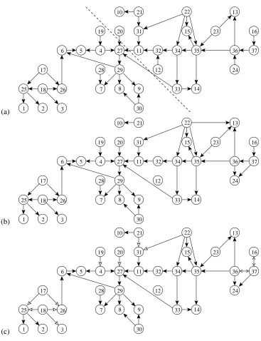
We have tested the summation and maximization algorithms on a small selection of data sets. The data sets contain discrete variables only and no values are missing. The Zoo data set is available from the UCI Machine Learning Repository (Blake and Merz, 1998, the data set contributed by Richard Forsyth). It contains 17 variables and 101 records. The Alarm data set built by (Herskovits, 1991) contains 37 variables and 20000 records, generated from the Alarm Monitoring System (Beinlich et al., 1989). In our experiments we used the first 100, 500, and 2500 records from the original Alarm data set.

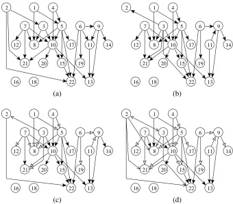
We also generated two new data sets. Both employ the binary parity function. The Parity1 data set contains 22 binary variables and 2500 records. We generated the data from a Bayesian network with structure as in Figure 4(a). The maximum in-degree is 4. The local distributions for each variable xi given its parents xGi were specified as follows. For each variable we associate a

fixed noise rateεi∈[0,1]. For each record x[t]we set xi[t] =xor(xGi[t])with probability 1−εiand

xi[t] =1−xor(xGi[t]) with probabilityεi. Here the parity function xor(z1, . . . ,zh) returns 1 if the

sum z1+· · ·+zh is odd and 0 if it is even. The idea behind using the parity function here is, of

20 21 15 22 10 17 12 11 19 13 16 18 9 6 5 3 7 8 14

2 1 4

20 21 15 22 10 17 12 11 19 13 16 18 9 6 5 3 7 8 14

2 1 4

(a) (b) 20 21 15 22 10 17 12 11 19 13 16 18 9 6 5 3 7 8 14

2 1 4

20 21 15 22 10 17 12 11 19 13 16 18 9 6 5 3 7 8 14

2 1 4

(c) (d)

Figure 4: Discovering network structure for Parity1. (a) The correct structure. (b) A structure that maximizes the posterior probability with 500 records. Posterior probabilities of edges with (c) 2500, and (d) 500 records. In (c) and (d) arrow headsN_,M_{, and}∧_{correspond to} intervals[0.99,1.00],[0.67,0.99), and[0.33,0.67), respectively.

were generated. In our experiments we also used prefixes of sizes 100 and 500 of the Parity1 and Parity2 data sets.

7.2 Model Specifications for Learning

In our experiments we used a simple generic Bayesian network model for structure discovery on the selected data sets. We used different values of the maximum in-degree for different data sets. For Zoo, Alarm, Parity1, and Parity2 the values were 6, 4, 5, and 3, respectively. Note that in the Alarm network (Figure 5(a)) the in-degree of node 27 is 4. We set qi(Ui) to be uniform and q0_i(Gi) to be proportional to 1/ n_|G−_i1_|

(for|Gi| ≤k). In the case of maximization we used the same

(a)

18 26

2 3 25

17

6 5 4

1 19 28 7 10 20 27 29 8 21 31 11 9 30 32 12 22 15 34 33 14 23 13 16 37 36 24 35 (b) 18 26 2 3 25 17

6 5 4

1 19 28 7 10 20 27 29 8 21 31 11 9 30 32 12 22 15 34 33 14 23 13 16 37 36 24 35 (c) 18 26 2 3 25 17

6 5 4

1 19 28 7 10 20 27 29 8 21 31 11 9 30 32 12 22 15 34 33 14 23 13 16 37 36 24 35

Figure 5: Discovering network structure for Alarm. (a) The correct structure. A dashed line sepa-rates two layers. For 2500 records, (b) a structure that maximizes the posterior probability, and (c) edge probabilities. Arrow headsN_,M_{, and∧correspond to intervals[0.99,1.00],} [0.67,0.99), and[0.33,0.67), respectively.

7.3 Results on Structure Discovery

For each data set we computed a single network structure that maximizes the posterior probability. We also computed posterior probabilities of edges for every pair of variables. That is, although the presented methodology supports computation of the posterior probabilities of arbitrary subgraphs, here we only consider directed edges. Here we show results for the data sets Parity1 and Alarm only. For the Zoo data set we are not aware of any correct structure, and for the Parity2 data set the results are similar to the results for the Parity1 data set.

Figure 4 illustrates possible end results of structure learning on the Parity1 data sets of different sizes. We see that with the data size of 500 records the best structure found (Figure 4(b)) is almost identical with the underlying correct network (Figure 4(a)). However, the edge between x2 and x3 is reversed and x3 has stolen the children of x2. This can be explained by a strong correlation

of x2 and x3. We also see that the underlying pattern of x6, x9, and x11 is just partly discovered.

With 2500 records there is some improvement: the correct direction between x2and x3is identified, x22 is correctly detected as a child of x2, and the incorrect edge from x3to x22is removed (results

not shown). This expected learning phenomenon can be observed in finer detail from the posterior probabilities of edges with the data sizes 500 and 2500 (Figure 4(c–d)). A small surprise is that with 2500 records the correct direction between x2and x3is less probable than the incorrect one.

Likewise, Figure 5 displays results of structure learning on the Alarm data sets of different sizes. We see that with 2500 records almost all correct edges were assigned a high probability and only few edges are added or are missing (meaning low posterior probabilities). An example of a missing edge is the one between the variables 12 and 37. That this edge is not supported by the data is in consistence with earlier studies on the Alarm data (e.g., Cooper and Herskovits, 1992).

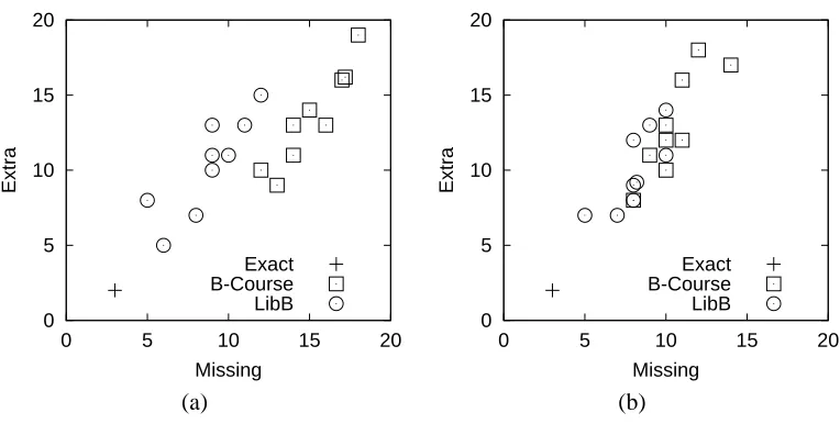
To investigate whether exact search for an optimal structure can really outperform heuristic search methods, we ran two freely available programs on the Parity1 data set with 2500 records and on its extended version with 10000 records. B-Course3 (Myllym¨aki et al., 2002) is a web-based tool for Bayesian network modeling. Among other features it implements a search algorithm for finding plausible network structures. Because the program runs on a web server, the time of a single trial is limited to 15 minutes (in real time). The user cannot change the parameters of the algorithm which combines greedy and stochastic search heuristics. LibB4 is a Bayesian network toolbox developed by Nir Friedman and Gal Elidan. It provides various search algorithms based on greedy and stochastic heuristics. Based on preliminary experiments we selected a greedy stochastic hill-climbing algorithm with 20 random restarts so that the time of a single run was about six minutes for the data set with 2500 records. (This is quite fair as our exact algorithm takes about nine minutes.) Since the algorithms implemented in B-Course and LibB are stochastic, we run both programs nine times. Each learned network structure was scored by comparing it against the correct structure. We counted the number of missing edges and the number of extra edges. A reversed edge does not contribute to these error counts if and only if the graph remains “locally equivalent”, that is, the correct graph is equivalent5 to a graph with the reversed edge. It is clear from the results, summarized in Figure 6, that finding an optimal structure is difficult for the tested heuristic methods. For these heuristic methods the number of errors is typically about four times greater than for the exact algorithm. That LibB performs better than B-Course might be explained by the fact that we

3. B-Course is available at http://b-course.cs.helsinki.fi/.

4. LibB is available at http://www.cs.huji.ac.il/labs/compbio/LibB/.

0 5 10 15 20

0 5 10 15 20

Extra

Missing Exact B-Course LibB

0 5 10 15 20

0 5 10 15 20

Extra

Missing Exact B-Course LibB

(a) (b)

Figure 6: The number of missing and extra edges in graphs found by the exact algorithm and two heuristic methods with nine independent runs each. Structures were learned from the Parity1 data set with (a) 2500 and (b) 10000 records. For visualization, coincident points are slightly perturbed. The correct structure has 31 edges.

made LibB to use many random restarts, whereas B-Course, perhaps, iterates over a single search chain; however, we do not know the actual search algorithm used by B-Course. Since the number of nodes, 22, is not very large and the optimization landscape is likely to be complex, using several random restarts may be a better strategy. Finally, it is worth noting that we did not set any in-degree bound for the heuristic methods. However, we compensated this by using the bound 5 for the exact algorithm, while the actual maximum in-degree is 4.

7.4 The Speed of Exact Structure Discovery

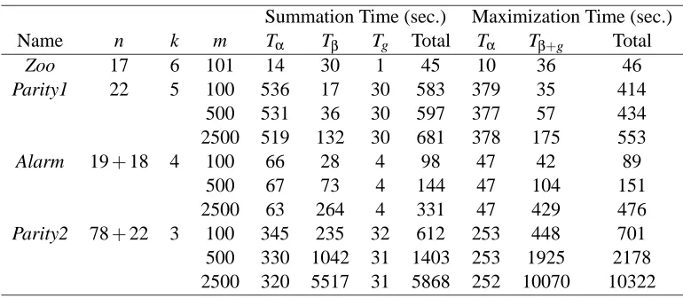
We also measured the speed of the implementation. To get a rather detailed picture of how the total time requirement is composed, separate measurements were carried out for a number of subrou-tines in the summation and maximization tasks. Table 1 summarizes the speed measurements over different data sets.

In the case of summation, Table 1 reports the time used for computing the functionsα,β, and g as defined in Equations (6), (8), and (7), respectively. We denote these three time requirements by T_α, T_β, and Tg. Recall that for Tα and Tg we have an exponential bound O(n2n) whereas for T_β we have a polynomial bound O(nk+1C(m)). When two layers were used (instead of one) the measurement was done for the functionα0expressed in the algorithm in Figure 3 (though reported as T_αfor convenience).

Summation Time (sec.) Maximization Time (sec.)

Name n k m T_α T_β Tg Total Tα Tβ+g Total

Zoo 17 6 101 14 30 1 45 10 36 46

Parity1 22 5 100 536 17 30 583 379 35 414

500 531 36 30 597 377 57 434

2500 519 132 30 681 378 175 553

Alarm 19+18 4 100 66 28 4 98 47 42 89

500 67 73 4 144 47 104 151

2500 63 264 4 331 47 429 476

Parity2 78+22 3 100 345 235 32 612 253 448 701

500 330 1042 31 1403 253 1925 2178

2500 320 5517 31 5868 252 10070 10322

Table 1: The speed of summation and maximization on selected data sets.

recompute some values of the functionsβ. That said, in this case the polynomial and exponential contribution are not easily told apart.

The experimental results are in good agreement with the presented asymptotic bounds. We see that the total time requirements are about the same for the summation and maximization tasks. Yet, Tα is consistently less for maximization than for summation. This is because of certain special numeric routines used for adding small numbers. That this difference is not preserved in the total time requirement can be explained by the fact that in the maximization some quantities are computed twice. We also observe that the relationship of the data size m and T_βis close to linear, as expected. (The slight distortion from linearity can be explained by the fact that when processing first hundreds records some expensive memory allocation routines are used.) Note also that T_α is invariant with respect to m.

Regarding the number of seconds needed for computing the probability of a feature, or, for finding an optimal network structure, it is clear that none of the combinations of model and data parameters used in our experiments lies close to the boundaries of practical tractability: the longest time is about three hours, for finding an optimal structure for the Parity2 data set with 2500 records. Yet, via the polynomial contribution, the time requirement is highly sensitive to the maximum in-degree k. For example, replacing k=3 by k=4 for the Parity2 data set would result in about 25-fold increase in the time requirement.6 Also, what is not explicit in the reported time requirements is that feature probabilities are usually computed for a large number of features; in our case, for every directed edge between two variables. Another important fact is that the space requirement of the implemented method is exponential: roughly n2nfloating point values need to be stored. This limits the use of the current implementation to at most 25 variables.

8. Concluding Remarks

We have presented a novel algorithm for learning Bayesian network structures from data. Our algorithm computes the exact posterior probability of a queried local subnetwork, e.g., a directed edge between two nodes. A modified version of the algorithm finds a global network structure

6. The increase is from 100₃

to 100₄

which maximizes the posterior probability. A major advantage of this method is that it explores all possible structures, still running “only” in an exponential time with respect to the number of network variables. We can expect that this feature makes it possible to successfully analyze cases where inexact methods may fail. Although we provided some bits of evidence for this hypothesis, more convincing validation would require a dedicated comparison study, not pursued in this paper. Here we, instead, reported a set of experiments to illustrate the presented methods and to investigate the actual speed of the implemented algorithms.

Our experiments demonstrate the applicability of the method. For moderate-size networks the running times were found to be feasible. The results also highlight the crucial role of the maxi-mum in-degree and the size of the data (i.e., the polynomial contribution) in the overall complexity. We also showed that structure discovery on large networks is practical if one can judge a suitable layering constraint on the space of network structures. Another main conclusion is that the actual bottleneck in the current implementation is the space requirement, not the speed. For example, a simple extrapolation (not shown) based on the speed measurements (shown in Table 1) reveals that a posterior maximizing structure for the Alarm data (37 variables, 2500 examples, maximum in-degree 4) could be found in about three days, if enough memory is present.

Although the presented algorithm shows promise as an exact method for structure discovery in complex Bayesian networks, there remain many important open problems. From the practical point of view, reducing the space complexity is a question of great importance. An open problem is whether the space requirement can be significantly reduced with little or no computational overhead. Interesting, yet rather theoretic, is the question whether there exists an algorithm faster than the one presented in this paper (asymptotically with respect to the number of variables). Since the maximization and summation problems resemble much the TSP problem and the computation of matrix permanents, respectively—for which no faster algorithms is known—we believe that the answer is negative.

There are many directions in which the presented methods can be extended. A practically important issue is handling missing observations; in this paper we only considered the case of complete data. The full Bayesian solution involves integration over the missing data. Unfortunately, it seems that exact computation is not feasible in general, unless the number of missing values is very small (less than 10, depending on the number of possible values of the variables). MCMC methods provide a practical way to overcome this problem. It is worth noting, however, that the exact summation algorithm readily applies to (posterior) prediction of the values of some variables, given data on the rest of the variables. A different issue is relaxing the structure discovery by allowing for undirected edges. In particular, instead of finding a directed graph that maximizes the posterior probability, one might be interested in searching for an equivalence class of such optimal graphs, conveniently expressed by a partially directed acyclic graph (PDAG); see, e.g., a recent paper by Castelo and Koˇcka (2003) and references therein. We note that an optimal PDAG can be found indirectly by first finding an optimal directed graph and then turning to its equivalence class. However, it is not clear how the presented algorithms could be used for computing feature probabilities on PDAGs, or whether the techniques used in our work can be extended to handle PDAGs in some more direct way.

a variable order, the latter factorizes the unconditional prior p(G). These assumptions are not only vital for efficient computation, but also offer a convenient and often suitable form for expressing prior beliefs. Nevertheless, modular priors can be criticized as the posterior distribution typically will not remain modular. A novelty in the work of Friedman and Koller (2003) was the introduction of a prior distribution p(≺)on orders; we took a small step further assuming that this distribution factorizes. Accordingly, the modeler should be able to think of a “true order”, which may be difficult if not unjustified. However, treating the order as a technical artifact without any interpretation re-moves the problem. Then the remaining problem is to justify the resulting form of the structure prior p(G). How well this form in practice matches the modeler’s prior is likely to be case-dependent.

In addition to the modularity assumption, we required that the number of parents of any variable is bounded by a constant. This is a convenient way to reduce the size of the search space. Unfor-tunately, only seldom is a small hard bound justified by background knowledge. However, under certain regularity assumptions one can argue that no variable should have more than about log₂m parents, where m is the data size (Bouckaert, 1994). This is because sufficient amount of evidence for many parents is needed to compensate the cost of model complexity. A similar result is due to H¨offgen (1993) who shows that about 2k data records are sufficient (maybe also needed) to learn Boolean networks, where each variable has at most k parents. These results—though rather obvious when ignoring the issues of accuracy and confidence—recognize that if the modeler’s background knowledge is vague, then a moderate in-degree bound is justified. On the other hand, it is worth noting that the algorithms presented in this paper work even if no in-degree bound is fixed. It is not difficult to see that then the time complexity is O(n2nC(m,n)), where C(m,n)is the time needed for computing a single local conditional marginal for m data records over at most n variables.

Acknowledgments

The authors thank Heikki Mannila for useful discussions and the anonymous reviewers for com-ments that helped to improve the manuscript. This work was partly supported and inspired by the Morgam (www.ktl.fi/morgam) and GenomeEUTwin (www.genomeutwin.org) projects.

References

S. Acid and L. de Campos. Searching for Bayesian network structures in the space of restricted acyclic partially directed graphs. Journal of Artificial Intelligence Research, 18:445–490, 2003.

S. M. Aji and R. J. McEliece. The generalized distributive law. IEEE Transactions on Information Theory, 46(2):325–343, 2000.

I. Beinlich, G. Suermondt, R. Chavez, and G. F. Cooper. The ALARM monitoring system. In J. Hunter, editor, Proceedings of the Second European Conference on Artificial Intelligence and Medicine, pages 247–256. Springer-Verlag, Berlin, 1989.

R. Bellman. Dynamic programming treatment of the travelling salesman problem. Journal of the ACM, 9:61–63, 1962.

R. R. Bouckaert. Properties of Bayesian belief network learning algorithms. In R. Lopez de Man-taras and D. Poole, editors, Proceedings of the Tenth Conference on Uncertainty in Artificial Intelligence, pages 102–109, Seattle, WA, 1994. Morgan Kaufmann, San Francisco, CA.

W. Buntine. Theory refinement on Bayesian networks. In B. D’Ambrosio, P. Smets, and P. Bonis-sone, editors, Proceedings of the Seventh Conference on Uncertainty in Artificial Intelligence, pages 52–60, Los Angeles, CA, 1991. Morgan Kaufmann, San Mateo, CA.

R. Castelo and T. Koˇcka. On inclusion-driven learning of Bayesian networks. Journal of Machine Learning Research, 4:527–574, 2003.

D. M. Chickering. Optimal structure indentification with greedy search. Journal of Machine Learn-ing Research, 3:507–554, 2002.

D. M. Chickering, D. Geiger, and D. Heckerman. Learning Bayesian networks: Search methods and experimental results. In Proceedings of the Fifth Conference on Artificial Intelligence and Statistics, pages 112–128. Society for Artificial Intelligence and Statistics, Ft. Lauderdale, 1995.

D. M. Chickering, D. Heckerman, and C. Meek. A Bayesian approach to learning Bayesian net-works with local structure. In D. Geiger and P. Shenoy, editors, Proceedings of the Thirteenth Conference on Uncertainty in Artificial Intelligence, pages 80–89, Providence, RI, 1997. Morgan Kaufmann, San Francisco, CA.

C. Chow and C. Liu. Approximating discrete probability distributions with dependence trees. IEEE Transactions on Information Theory, 14:462–467, 1968.

G. F. Cooper and E. Herskovits. A Bayesian method for the induction of probabilistic networks from data. Machine Learning, 9:309–347, 1992.

R. Dechter. Bucket elimination: A unifying framework for reasoning. Artificial Intelligence, 113 (1-2):41–85, 1999.

N. Friedman and D. Koller. Being Bayesian about network structure: A Bayesian approach to structure discovery in Bayesian networks. Machine Learning, 50(1–2):95–125, 2003.

A. E. Gelfand and A. F. M. Smith. Sampling-based approaches to calculating marginal densities. Journal of the American Statistical Association, 85:398–409, 1990.

D. Heckerman, D. Geiger, and D. M. Chickering. Learning Bayesian networks: The combination of knowledge and statistical data. Machine Learning, 20:197–243, 1995a.

D. Heckerman, A. Mamdani, and M. P. Wellman. Real-world applications of Bayesian networks. Communications of the ACM, 38(3):24–30, 1995b.

D. Heckerman, C. Meek, and G. F. Cooper. A Bayesian approach to causal discovery. In C. Gly-mour and G. F. Cooper, editors, Computation, Causation, Discovery, pages 141–165. MIT Press, Cambridge, 1999.

K.-U. H¨offgen. Learning and robust learning of product distributions. In Proceedings of the Sixth Annual Conference on Computational Learning Theory, pages 77–83, Santa Cruz, CA, USA, 1993. ACM Press.

R. Kennes and P. Smets. Computational aspects of the M ¨obius transformation. In P. B. Bonissone, M. Henrion, L. N. Kanal, and J. F. Lemmer, editors, Uncertainty in Artificial Intelligence 6, pages 401–416. North-Holland, Amsterdam, 1991.

P. Larra˜naga, C. Kuijpers, R. Murga, and Y. Yurramendi. Learning Bayesian network structures by searching for the best ordering with genetic algorithms. IEEE Transactions on Systems, Man, and Cybernetics, 26(4):487–493, 1996.

S. L. Lauritzen and F. V. Jensen. Local computation with valuations from a commutative semigroup. Annals of Mathematics and Artificial Intelligence, 21(1):51–69, 1997.

D. Madigan and J. York. Bayesian graphical models for discrete data. International Statistical Review, 63:215–232, 1995.

P. Myllym¨aki, T. Silander, H. Tirri, and P. Uronen. B-Course: A web-based tool for Bayesian and causal data analysis. International Journal on Artificial Intelligence Tools, 11(3):369–387, 2002.

J. Pearl. Causality: Models, Reasoning, and Inference. Cambridge University Press, Cambridge, 2000.