Application of the element potential method to gaseous chemical equilibrium calculation

TO GASEOUS CHEMICAL EQUILIBRIUM CALCULATION

Thesis by

Joseph Richard Wrobel

In Partial Fulfillment of the Requirements For the Degree of

Mechanical Engineer

California Institute of Technology Pasadena, California

ABSTRACT

I wish to extend my grateful appreciation to the research advisor, Dr. Paul J. Blatz, for his sincere

interest and capable guidance throughout the prosecu-tion of this work.

A special acknowledgement is due the National Aeronautics and Space Administration for financial

assistance rendered through the tuition support program of the Jet Propulsion Laboratory of the California

Institute of Technology.

I extend my thanks to my wife, Janice, for her con-siderable effort in preparing the typescript of this

SUHMARY

The equilibrium state of a mixture of chemically react-ing perfect gases is described by the application of the maximization of entropy principle for the case of fixed

enthalpy, pressure, and atomic specie mole numbers. The conditions at equilibrium are formulated in terms of the Massieu element potentials and the temperature; there being

one element potential for each distinct atomic type in the mixture.

An iterative method of relaxing the element potentials and the temperature to their respective equilibrium values is presented. The exponential dependence of the partial pressures upon the potentials and the logarithmic form that is selected for the temperature guarantee the non-negativity of pressure and temperature at each step in the iteration. A stability criterion based upon the concavity of the

entropy function in the variable space is developed as an aid to obtain rapid convergence. Since the number of atomic types is, in general, less than the number of molecular s pe-cies considered in the reaction, the rank of the solution matrix is less than that for solution methods not using the

PART

I II III

IV

v

VI

VII

VIII IX

X

TABLE OF CONTENTS

TITLE PAGE

Introduction 1

Description of the Equilibrium State 3 An Iterative Solution Technique

8

The Stability of the Equilibrium State

13

Convergence of the Solution

Application of the Element Potential Method to the Equilibrium Determination of the Nitrogen Tetroxide-Hydrazine

Combustion System

An Estimate of Trace Molecular Species and a Test for Condensed Phases

17

21

28

Extension to Psuedo-Equilibrium Stat es

30

Extending the Solution

32

Conclusions

46

Nomenclature

47

References

49

Part I

INTRODUCTION

The determination of the state of thermodynamic equi-librium for a chemically reacting gas mixture of fixed total

enthalpy is a problem of daily occurrence in the field of

chemical rocketry. The problem is readily resolved to that of determining the solution to a set of non-linear algebraic equations by an iterative method. The thermodynamic formu -lation of the problem determines the character of these equations, and therefore greatly influences the complexity of obtaining a solution. Through the years a considerable number of approaches have been presented, both in the thermo-dynamic formulation and in the solution technique. The

methods of

(1)-(3)*

are representative of these. The

fore-most complicating feature of the problem is the demand that the formulation and solution technique be sufficiently gen-eral to permit rapid convergence to the equilibrium state from arbitrary initial parameter estimates. The present

approach is a simple, yet exact and general, thermodynamic formulation coupled with a solution technique possessing a

thermodynamic criterion of solution stability, a minimum

number of iterated variables, and a method for determining starting values requiring only the estimation of the thermo

-dynamic temperature. The approach is quite amenable to

- 2

-either hand calculation or digital computation on small

Part II

DESCRIPTION OF THE EQUILIBRiill1 STATE*

To begin, a closed system is defined. The concept of

closure is defined with respect to heat transfer, mass

trans-fer, and all types of work. For this analysis the types of

work are restricted to hydrostatic mechanical work. The

system is composed of an assembly of gaseous, chemically

reacting molecules. Such a system may be completely speci-fied by assigning: an extensive parameter to the lumped

internal degrees of freedom, the interal energy (U); an

extensive parameter to the geometric degrees of freedom, the

volume (V); and a set of extensive parameters to the chemical

degrees of freedom, the mole numbers (Ni)• The subscript 1

ranges from 1 to C, the number of discreet molecular species

in the mixture. The differential parameter dU is a measure

of the heat transfer to the internal degrees of freedom of

the molecular species. The differential parameter dV is a

measure of the hydrostatic work done on or by the system.

The differential parameters dNi are a measure of the mass

transfer to or from the system.

For the system described in the preceeding, we may

postulate the entropy function (S), which possesses the

following properties:

a. S is a continuous and differentiable function of

the extensive parameters.

*Portions of this development have been abstracted from

4

-b. S is a monotonically increasing function of

u.

c. S is a maximum in the equilibrium state.

d.

s

approaches the limit zero as

(

au)

-as

v) N;.. approaches zero.

If we further define the derivatives with respect to

the ext ensive parameter as follows,

l~~)y

N·

I

(la. )

-T )

..

(as)

_

p _(lb.)

aV

u,N~ = T

(

;~t

.

v

,

Nr::

-

)!:_

;.

(lc.) T

we arrive at the differential form of the entropy function

dS

=

du

+

_e_

dv -

.z:

f!.

;

dN.i

T T .i T

(2)

Callen (5) illustrates that these properties of the entropy

function are compatible with the conventional statements of

the laws of thermodynamics. The resulting postulatory form

of the entropy function is, of course, identical with the

phenomenalogical formulation of Gibbs

(6)

.

In a chemically reacting system, the concept of closure

with respect to mass transfer requires the preservation of

atomic species. The conservation of atoms di ctates that

where:

"'

a. w i is the number of a toms of type o< in molecu-lar species i

b. the total number of types of atomic species is equal to A

c. N oc is the number of gram a toms of type ex per unit mass of system.

The N oC possess the property that

(4)

where A"' is the atomic weight of atomic species <X • The total mass of the system is taken to be unity.

In the light of these definitions, consider the differ -ential form of the entropy function for a process in which the enthalpy and pressure are to remain fixed, i .e.,

dH

=

d. (

U

+

PV)

=

o

clP

=

0

(5a

.

)

(5b. )

The differential form of the entropy function (equation 2) becomes

d

5

=

d.

(

U

+

PV)

T

0

_ VdP

T

0

(6)

In the equilibrium state S is to be a maximum and therefore for a virtual process dS shall be zero, subject to the mass

6

-multipliers* is applied. Define the new function

¢

,

(7)

\o(

where the A are the constant Lagrange multipliers, one for each atomic species constraint. Optimizing the

s6

function with respect to the composition variables evolves equation

8.

ad;

(8)

-The entropy derivatives are evaluated from the postulated properties of the entropy function presented in equation 1.

From the mass balance constraints of equation

3,

the composition derivatives are obtained, i.e.,

dN(. ·

woL

_,... (9)

Therefore, for each molecular specie in the mixture at the

equilibrium state, the substitution of equations

8

and

9

into equation 6 reveals that

(10)

The same result is obtained for fixed U and

v.

The chemical.

Massieu potential (~i/T) of molecular species i existing in the equilibrium mixture can be decomposed into Massieu element potentials AtJ{, , there being one element potential for each atomic species o( • For example, at equilibrium

J!:.f.lz,O

-

'A+

zX'

(lla.)

T

}::icoz. =

>-'

+

z>..o

(llb.)

T

To determine the maximum value of the entropy, subject

to the constraints, equation 10 is multiplied through by

Ni and summed over 1

However, since

and

¢

==

s

+

.:£

)...CJ("tvo{_

=

s

+

Fir

0(.

F

T

jj_-

s

T

the value of the entropy in the equilibrium state is

S

==

J:L -

2

t

NoL

T

"

(12)

(13)

(14)

(15)

The equilibrium state is specified in terms of the A + 1

quanti ties [ A01} , T. It is proposed that the solution of

the equilibrium problem be performed by relaxing {

Xj

and

T by an iterative technique to their respective equilibrium

values. This amounts to the solution of a constrained

maximum problem by iteration upon the Lagrange multipliers,

which take on the identity of element potentials for this

problem. It shall be illustrated that starting values of the parameters are easily estimated and rapidly relaxed to

- 8

-Part III

AN ITERATIVE SOLUTION TECHNIQUE

A relaxation procedure ror determining the equilibrium state is now presented for the system under study. The

enthalpy of such a perrect gas mixture, at equilibrium, shall be equal to the specified enthalpy H, as in equation

16.

1-1 -

z

_.

N·

_"- ~· _).. =

o

,(.

(16)

The mass balance constraints require that

{ N«j - {

f

~·

w:}

==

0

(17)

The equilibrium state is described by the element potentials, as in equation

18.

&

(18)

T

Here ~+ is the standard free energy of molecular specie i at temperature T, and p+ is the standard pressure, usually

taken to be 1 atmosphere. The remaining relation to be

applied is that relating the partial pressures to the mole

fractions for perfect gases; the Gibbs-Dalton Law of equation

19.

N·

_{h .}

). - ~A.

- - -

N

p

(19)

where N, the total number of moles, is defined as N = ~ Ni•

...:

Among these equations, the mole numbers may be eliminated at the outset by ratioing, i.e.,

N<

=

H

rvz

f:J:/p

w.<.<l(.

N

Z.

A/

P

ft.;.

To abbreviate the notation, it is convenient to define an

averaging operation

<

j':

>

=

~

p;;

P

xi

I.

Equation 20 may then be abbreviated to

N"-_

1-1

For the pressure constraint, equation 22 applies.

$

p;;

p

=

I

=

<I>

I.

(21)

(22)

The antilog of equation 18 presents the partial pressures

explicitly in equation 23.

k

=

_r

~

[ z

~ol.-

P-/

J

p

p

I ( ~ RT

(23)

For a given estimate of

{A:}&

Tn, where subscript g implies

the n'th estimate, errors will occur in the enthalpy, mass

balance and pressure unless the equilibrium values were

estimated precisely. These errors result in an imbalance,

or residual, in the various constraint equations. Define

the following functions for each iteration

(24a.)

In the equilibrium state, the~ 's are all zero. The

6 n's represent the dimensionless residuals in the

10

-relax the selected functions to zero by the Newton-Raphson

method of linearized differential corrections, i.e.,

0

=

d

+

(dLl~)

&Tn

+

(d

f~tn) bA~

n

dT

d

f.~

(25a.)

(25b.)

o(

It should be noted in passing that the ~ 's could also be

f ormulated from equation 21 as

and still retain the non-dimensionality.

The

~Tn

and

[SA~}

represent the first order correc -tions to T and

[~o(}

r espectively to obtain the desired zeros.

From this point on the dummy subscript/superscript ~ shall

imply a general atomic species 1 ~

ft

~ A. The various par -tial derivatives are evaluated at parameter values appro -priate to the n'th estimate. The first order corrections are determined by the inversion of the resulting A + 1 linear simultaneous relations.

The partial derivatives are obtained from the defining relations of the ~

's,

{)!;

/==E._

[<I>

-J]

==

<'i1

>

oT

dT

RTz

-;;;t!

=

_£_

[<'>-I

]

=

<wo<.>

()>/

d~(3 R.

df1c~.-= ~

[No(<~>

-J]

==

No([

(

~

z'>

+

<ce>

J T dT H

<

we(

>

H R. (ur'> Tz <wt!()

-

<~> <wo(~>

]

<w"'i

'

R.Tz

(26a.)

(26b.)

(26d.)

The various averages are computed using the partial pressures predicted by equation 23 with the n'th estimates. Substitu

-ting the derivatives of equations 26 into equation 25 and

transposing the constfu~ts results in equation 27.

<

'-R.

'>~ dT~

- -

+

(27a.)

RT'V1. T )"\.

_

6~

=

N~R~

[

<c

f

>-K

f-

<_-f?tz),.

_

(fz?.,._(w,('t..'>

jSTn

(27b. )

H

<w~

If

R1..r;_.z.. (w"'~ 1?.2~2 ...,_ T-w.

-f

N~

"-'>

[<-It

WI~

- (--Pt

>

~

<

Wo(~t'>n]

J}

~

H UJ /?t <wll(>.,. /V

Upon inverting this system, the parameters for the (n + l)'st estimate are arrived at by adding the corrections to the

n'th estimates, i .e.,

(28a. )

( 28b. )

The exponential form of T is selected to insure only positive

temperatures. In the limit of small values of bTn/Tn this

reduces to simple additivity of the linear correction. The

exponential dependence of Pi upon {A~} guarantees the non

-negativity of pressure.

The linearized iteration scheme described in the pre

- 12

-of the series expansion remain small. ~nis may not always

Part IV

THE STABILITY OF THE EQUILIBRIUH STATE

In order to establish that the optimized solution is a

maximum, the entropy function must be concave in the region.

This requires that, for a virtual displacement of the system

from the converged solution, the first order change of

en-tropy must be zero and the second order change must be

nega-tive. To evaluate the second order change it is necessary

to return to the constrained optimum problem. Consider an

optimizing function

(29)

{ 'o(}

where 1\ are the Lagrange multipliers for the atomic

specie constraints and ~ the multiplier for the constrained enthalpy. The constraint equations are as follows,

P=P

(30a.)

H

=

_{~ ~} <'

N

ft.

.(.

J.

( 30b.)

(JOe.)

Given the entropy flli~ction in t erms of temperature, pressure,

and mole numbers for a mixture of perfect gases, i.e.

equa-tion 31,

5

=

z

N~

ft.; -

2

/1£

·

ur-

NR.

kNf_E_)-

<

N:

Riht.N.- (31)

. - . ~ J-.r L. ,( A.

). T 4

T

~ i

-

14-the

¢

1 ftmc ti on may be expressed explicitly.

*N~

·

iL(-

z

ry;,/ _

NRk(%+)-

t

~

.

Rh~

·

T

~

T

I ~

(32)

-1-

NR

b.

N-

(/J

~

~·-h

,;

+

:Z

~ Ao~- ~

·

U1

o{.

~ ~ ~

-1.'

To a quadratic approximation, the variation in ~ is given

by

(33)

~

~·C;~·

( ; - (//)

+

~

[-l(

(

f

-Cj

)-r

~o(X'--jf+

A A

-

R.

iM{~-t)

1-

R.

~N-

ICPn

/~.(.·]

.f

~·

-

~

M·CL/ (

Sr)

2 +

$~·

(

; -

f.b)

Jr

JN;·

, Z T •

+

!G

~l-

8.

2

(JN..lz.

i?J fV

,z _,·

ft{

Applying the principle that the first order variations must be independently zero, the previously formulated equilibrium conditions are repeated, i.e.,

Z.'

)..

o(

w{

c~.. = + jJ~./r

0(

Sm

₄

x

= J-1 -

2

Aci.No(,

T

ot

and the Lagrange multiplier

lf

becomes the inverse of

tem-perature. The quadratic variation must be negative in sum, if the optimized state is truly a maximum. The remaining

quadratic terms of the variation, therefore, must obey the inequality of equation

34.

The mole numbers may be eliminated from equation

34

by apply-ing equation 19 and its variation. The substitution into equation

34

produces the new inequality of equation

35.

(3.5)

The inequality of equation

35

may be cast in terms of the element potentials by substituting from the variation of equation 18, i.e.,

<w

,

1

>

~)#

+

_(-ft.>

J--tnr

(36)

R RT

and noting that, in equilibrium, the number of moles may be expressed in terms of the enthalpy as follows

(37)

therefore:

&_

= -

f

{!{> = -

<c

e

>fr

_

g

!p_

~

N

<-A

>

(-A>

i P-~· (--!{

>

(38)

The result of the substitution is presented in equation

39.

(39)

The inequality of equation

39

is of value in determining whether a given set of parameter estimates will readily

16

-a line-arized iteration technique, since it contains the

thermodynamic constraint upon second variations.

If the linearized corrections to the solution

parame-ters [~}, T do not satisfy equation

3

9

,

it is apparent

that the starting estimates were made in a region of the

variable space that does not possess the correct curvature

to describe a maximum. It may be more efficient to

re-estimate than to extrapolate from the initial point, for the

entropy surface may not be amenable to a linear fit when far

from equilibrium. The coefficients of equation

39

should

be evaluated at the equilibrium condition. This is not

known a priori, and the estimated properties must be

substi-tuted. This lessens the effectiveness of equation

39

as a

calculation aid. However, this is a good a posteriori check

of the estimate method developed. A further discussion of

this point is presented in Part VI when numerical results

Part V

CONVERGENCE OF THE SOLUTION

The application of a linearized iterative technique cannot guarantee unconditional convergence to the equi-librium solution. The thermodynamic stability criterion discussed in Part IV is a convenient discriminator for

first estimates and gives an indication of the thermodynamic influence upon solution convergence, but is admittedly cum-bersome for evaluation at each step. It is convenient to introduce some measure of the total error in the solution to judge the progress of successive iterations and determine when the solution has essentially converged. This can reduce the number of iterations to convergence by indicating the most efficacious path of relaxation. In the linearized scheme, the slopes of the ~ functions are extended in the various coordinat e directions from the estimated point. Due to curvature of the function, the linear extension departs from the true dependence. Because of this departure it may be expected that the direction of the change is approximately correct, but that the magnitude of the correction vector may be incorrect. If the proposed linearization is a good esti-mate of the actual dependence, the optimum correction vector magnitude will approach the predicted magnitude. The optimum magnitude is that which minimizes the errors ~p and {Ll~} _•

P _{

/\o(}

18

-normalized. The normalization permits comparison of the

errors with unity to determine an absolute measure of convergence.

The optimization is a one-dimensional one resulting in

the proportion of the predicted correction magnitude which results in the minimum error. A logical choice for the

error function to be minimized is the sum of the squares of

the

L

P and [

~}

• Define the error at the n'th iteration to be

(dn)

2

+

£

1

(6n):G

oL

If the iterative scheme is to be convergent, subsequent errors should be monotonically decreasing, i.e., E2_L

1<E2 <E2 ₁•

n..- n

n-After inverting the correction matrix for the n'th iteration one obtains the linear corrections blnTn and

parameters to be used to calculate the properties at the

n + l'st iteration are therefore

(4la.)

(4lb.)

In order to minimize the number of iterations required, it is desirable to select

7T

n such that the error at the start

of then+ l'st iteration is a minimum. This requires the

This implicit function of

TT

n is most easily optimized by a graphical determination. For each value of 71 n' the

function must be evaluated. After each iteration this opti-mization must be repeated. The number of iterations, and

therefore, the number of matrix inversions, may be reduced

at the expense of more matrix multiplications and

manipula-tions. This inconvenience can be minimized by recognizing that the optimization need be only approximate.

tant criterion is that the subsequent error E~ +

smaller than

E~.

Therefore, if one evaluates

E~

"n = 1, assuming the linear correction technique exact, and finds it less than

E~,

the convergence

The impor

-1 be

+ 1 for

to be

is assured

and the next iteration may be started. Note that the

compo-c~..

nents .£0. P and

.:d

must be computed for the next iteration

matrix anyway. If E_n 2 _{+ 1}

(7Tn

= 1) is not less than En2 '

then one may select other values of ZTn and determine the corresponding error. A choice of

7Tn

=

0.5

will give a third

2

point, and the trend of En +

1 should be apparent, at least in approximation.

It must be noted that, although the errors ~p and ~~ are dimensionless they may have a disproportionate influence upon the combined error E2• In particular, the enthalpy

CJ(._

20

-The enthalpy is a relative property. A gas mixture may,

depending upon the datum selected, possess either a negative

or a positive value of H. This may "sensitize" the error

function to small changes in enthalpy since, for small

(-A.'>.

changes in parameters, H can undergo order of magnitude

changes as well as sign changes. One could, with sufficient

substantiating experience, assign weighting coefficients in

the error function formulation to account for these

inequi-ties and define an error function of the type

(43)

It will be demonstrated numerically that the selection of

the enthalpy base implicitly defines such a biasing. The

enthalpy base which permits negative as well as positive

values and has its zero in the range such that H is small in

magnitude represents the most discriminating one with respect

to enthalpy errors.

The iterative method fails for H

=

0, due to the

singu-oi..

lari ty introduced in the definition of

IS. •

Although such

instances are rare, this dependence upon the enthalpy datum

is somewhat disconcerting. It is generally accepted that

one may assign an arbitrary datum for enthalpy measurement.

However, the present difficulty is primarily one of

defini-tions. In Part IX a more fundamental pr oblem with respect

Part VI

APPLICATION OF THE E~mNT POTENTIAL ~ffiTHOD TO THE

EQUILIBRIUM DETERMINATION OF THE

NITROGEN TETROXIDE-HYDRAZINE COMBUSTION SYST~~

To demonstrate the appli cation of the calculation method

described, a typical solution is presented. The chemical

system selected is that of nitrogen tetroxide (N₂

o

4) and hydrazine (N

2

~) in a mass mixture ratio (0/F) of 1.2:1.

The combustion is assumed to occur at 150 psia. This system

is a convenient example in that t he equilibrium solution is

available from independent calculations for comparison

purposes. From these assumptions, and the properties of

the reactants, the [N~J

and

H

may be determined as follows:

The masses of the separate reactant s are

mass of N_2\ =

t

₊ 1 _1.2 = 0.4545 gr./gr. mixture

1.2 ₌

0.5455

_{gr./gr. mixture}

t

+ 1.2

The moles of reactants are computed, using the molecular

weights of t he reactants, to be

moles of N₂

1\

= 0.4545 = 0.014183 mo1./gr. mixture

32.048

0

·5455

_{= 0.005928 mol./gr. mixture}

92.016

- 22

-NH = 4(0.014183) = 0.05673 gr. at./gr. mixture

NN

=

2(0.014183) + 2(0.005928)

=

0.04022 gr.at./gr.

mixture

N° = 4(0.005928 = 0.02371 gr. at./gr. mixture

The mixture enthalpy is determined from the assigned enthalpy*

of the reactant mixture at the input conditions (298° K

assumed)

h(N204) = -.578 Kcal. /mol.

h(N2

B4)

= 18.170 Kcal./mol.

H = (0.005928)x(-.578) + (0.014183)x(l8.17) = .2543

Kcal. /gr. mixture

= 254.3 cal./gr. mixture

This completes the determination of the equilibrium con-atrainta.

The first estimate of combustion temperature is selected

to be 2500° K., approximately 500 K0 leas than the established

equilibrium value,9) This was selected as being representative

of the uncertainty in temperature of an unexplored system.

Appendix I contains the method of determining the first

esti-mates of

{Aj

from the assumed temperature. The potentials

are estimated to be,

}I

)l,jR

-

-

q,q/

)..~I

R =: -/Z. 9Z

)..~I

R

=: - !8.06

Using these values for the potentials at 2500° K, the vector of partial pressures of the molecular species is computed from equation 23. The various coefficients of equation 27 are evaluated using the partial pressure averaging tecP_nique. The resulting

4

simultaneous linear correction equations are then solved. The first order corrections are made to [ A.'o<"} and T and a new composition vector computed. The results of the first three iterations are presented in Table I . The

r/. d..

root of the error function ( -fi2) and the function

.!!

-

Z)... ~

RT o<. .n are presented as well, the latter is identically the entropy

-24-Table I

RESULTS OF THE EQUILIBRiill1 CALCULATION FOR THE CONi3USTION

OF N204 - N2B4 AT 150 PSIA AND 0/F = 1.2:1

,\H/R _AN/R AO/R

T

(°K)

I[E2

li->tif

RT R

Zero

Estimate (elemental

products) -9.12 -13.03 -14.22

2500

715.0 1.430

First

Estimate -9.91 -12.92 -18.06

2500

3.50

1.560

1st

Iteration

Second

Estimate -9.63 -13.20 -18.00 2857 0.561 1.546 2nd

Iteration

Third

Estimate -9.97 -13.29 -17.14 2975 0.310 1.550

3rd

Iteration

Fourth

Estimate -10.10 -13.31 -16.84

3025

O.J.41 1.550 Independent

The results presented are for iterations in which the

full first order corrections were applied. It is worthwhile

to note that the error 1JE2 is monotonically decreasing for

n

this system. To determine any departure from the optimal

iterative steps, the error was evaluated for intermediate

cases, i .e., fractional first order corrections. In all cases, the linear step appeared to be approximately optimum.

A solution using precisely optimum iteration steps was not performed. The results of this survey are presented in

Table II, for the sample calculation at the first and second iterative step.

Table II

OPTIMIZATION OF THE ITERATIVE PATH

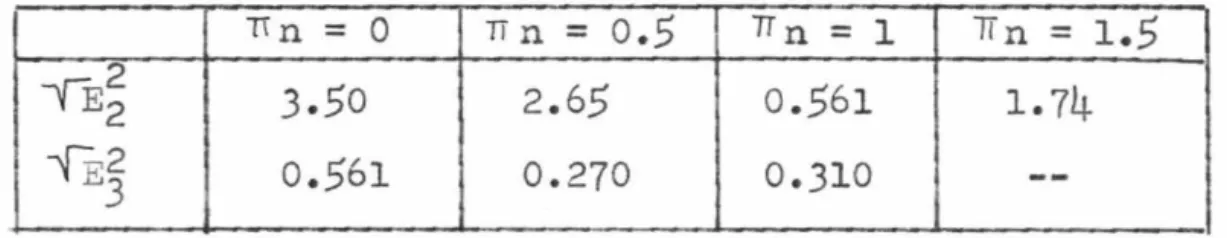
Tin = 0 Tin= 0.5 Tin = 1 1Tn = 1.5

"'lE2

2 3.50 2.65 0.561 1.74

fE2

3 0.561 0.270 0.310

--These results point up the practical efficiency of using the full predicted step between iterations, provided that the

error is decreasing.

In defining the error function (E2), it was noted that the magnitude of the function is dependent upon the enthalpy base selected. The dependence of the magnitude of the error at the initial estimate upon the base selected has been

26

-compounds at 0° K such that virtually all other molecular species possess positive enthalpies. In (8) zero enthalpy is assigned to the elements at 0° K. In

(10)

the elements are assigned zero enthalpy at standard temperature (298° K). It is apparent that, in the order presented, the reference bases tend to smaller algebraic enthalpies for a given species.

The values of the mixture enthalpy computed from the prescribed reactant enthalpies for the iterative example are,

2224

cal./gr. ,

254

.

3

cal./gr. and

130

.

6

cal./gr. respective -ly, for the three enthalpy reference systems mentioned. The corresponding errors at the first iteration (

lfE

₁2 ) were

0.48,

3

.

50,

and

8

.

18

respectively. This illustrates that the error function described can assume different values for the same estimate, depending upon the enthalpy reference. This scale change does not alter the normalization or dimen-sionality of the error function. It merely serves to accen-tuate small enthalpy errors.

criterion may be applied to determine the adequacy of the estimates at various levels of temperature error.

The equilibrium value of the temperature is

3055°

K. The inequality of equation

39

was tested at 2000° K, 2500° K,

- 28

-Part VII

AN ESTII'iATE OF TRACE iviOLECULAR SPECIES AND

A TEST FOR CONDENSED PHASES

The analysis presented will determine the equilibrium

state of maximum entropy for a specified set of molecular

species assumed to be present in the mixture. For the sake

of brevity, only a portion of the possible molecular species

are considered in the equilibrium determination because of

the vanishingly small mole fractions, and therefore influ

-ence, of certain molecular forms in a given region of tem

-perature. The rank of the correction matrix is unaffected

by the number of molecular species considered. However, the

vector multiplications represented by the coefficients of the

matrix become operationally more cumbersome to perform because

of the number of components involved. This implies that an

appreciable calculation effort may be expended needlessly by

considering trace species. A procedure for avoiding this is described in the following.

At each step in the iteration, the mole fraction of all

possible molecular species may be evaluated from the esti

-mated parameters to be

h ·

+

[

\# .f3

JJ+-_r)

=

!:li_

=

K

~ ~,4 - £::::L ]

p

N

p

R R-T

Those species exhibiting a value less than some arbitrary

level, e.g. 10-4 to 10-5 should be neglected in the succeeding

on the basis of a mole fraction average, and therefore

coef-ficienGs computed for the truncated species distribution

will assymptotically approach the values computed

consider-ing all possible species. At convergence, when the error

has been reduced to an arbitrarily small value, the parame

-[x

d..},

ters T are assymptotically approaching the exact

values, and the partial pressures of trace species predicted

from these parameters are essentially correct. The resultant

mismatch in constraints

[N~},

H,

P

,

should remain

negli-gible. This mismatch may readily be determined if desired.

This procedure may be used to predict the presence of

condensed phases as well, although only qualitatively at

present. A gaseous molecular specie may represent the vapor

phase of a possible condensed phase. Although only perfect

gases have been considered in the iterative scheme, the

under-lying analysis is applicable to condensed phases. The chemi

-cal potential (;Ui) of the gaseous phase of a molecular

species is, in the equilibrium state, equal to

The molal chemical potential of a pure, ideal condensed

phase is only a function of temperature, and is tabulated.

Therefore, if the value of the chemical potential of the

con-densed phase of molecule i at the converged temperature T is

less than the gaseous phase potential computed from

Tz

>..~~""-,

d.

the condensed phase is present in some unspecified amount,

and the solution must be re-evaluated, taking into account

the phase or phases predicted. This recomputation has not

30

-Part VIII

EXTENSION TO PSUEDO-EQUILIBRIID1 STATES

The ~~alysis presented is valid for predicting the

state of equilibrium obtained by a mixture of reacting gases given time for all kinetic processes to subside, or come into balance. In a dynamic process it may be desired to determine the psuedo-equilibrium state in which certain, or

all, of the molecular species are "frozen" at specified

molal levels not necessarily those of the maximum entropy state. ?ne iterative scheme may be applied to such systems to determine the adiabatic temperature and unspecified

molecular specie mole numbers. This requires the introduc

-tion of the new constraint(s) that N i shall be a constant equal to the specified value for the frozen components.

~ is a dummy variable representing the frozen specie ~

.(

The composition vector

Wj

is replaced by one which has a

Here

•

zero component for all but~=~ , for which the component is unity. This specification increases the number of variables to be iterated by one for every added constraint. In effect,

the frozen molecular species are treated as inert, irreducible atomic species. The effect of the additional constraints is

to uncouple the correction equations, and results in numerous zeros in the correction matrix.

cases, the molecular specie in question is introduced both as a psuedo-inert atomic specie and as a conventional product.

32

-Part IX

EXTENDING THE SOLUTION

Once the equilibrium solution has been obtained for a

set of constraints P,

tNfH}

,

it may be desired to determine

the influence of small changes in these constraints upon the

equilibrium state. In particular, the solution at another

pressure or enthalpy may be desired. The linear correction

equations represent a perturbation procedure for just such

changes • The functions Ll P, {

E}

,

defined as the error

com-ponents in the iterative calculation take on values

appro-priate to the perturbed constraints. A solution of the

resulting simultaneous equations determines the linear

per-turbation of the parameters

[fJ,

T, and permits an

approxi-mation of the new equilibrium state. The new constraints

P1 , N~' , H1 _{prescribe the new values of the} ~ _{'s as}

follows.

The linearized perturbation equations are

0

=

t6p'

+

(44a.)

The errors, or residuals, are to be made zero in the new

equilibrium state. The b.P', [~-<'J are defined using the new constraints, i.e.,

J

(1

>

-I

=- p

(1>-!

p'

<'

n) - I

H'

(w•>'

p

p' N-<'(~'>

-I=

N~'(-j,_)-

I

p' P H 1

<

w-<> H I

<

w-<)

(45b.)

The necessary derivatives are the same as those computed

in the iterative scheme, except that all of the primed

constraints are substituted. The resulting perturbation

equations are therefore

(46a.)

(46b.)

This set of equations may be simplified by noting that P

P'

may be factored, and that the following relations are

appropriate at the point from which the perturbation is

made

( wol..') ==

N""-(1{>

H

A further abbreviation is possible by noting that for small

changes in the variables

p

~ ? -"--' p

o('j .. tc<' /} I

I

-

N

I

1-1' -::::: - ~ e!.-.

+

-»n ::

34

-Including these simplifications and abbreviations into the perturbation equations yields

(47a.)

(4

7b.)

The presence of the primed quantities in the correction matrix would constitute a second order correction in the solution, and consequently they have been replaced by the base values. All other second order terms have been dropped in the linearization. Also, retaining the primed quantities would require the re-evaluation of the correction matrix at each perturbation. By this method, the solution may be extended from a known point to obtain approximations of the parameters appropriat e to the new equilibrium state for constraints P', H1 , [N~'} • Again it must be cautioned that the enthalpy base selection may influence the accuracy when working with H and/or H' nearly zero.

Two numerical examples have been evaluated to illus-trate the application of such a perturbation technique.

for the 1.2:1 mixture ratio, nitrogen tetroxide-hydrazine system. These were compared with the values obtained by an independent exact solution.(9) The base point was at a pressure of 150 psia. The comparison was made for

pres-sures from

5

psia to 160 psia. Further data for comparison was not conveniently available. The 6"'- 1 _{s are zero, since} enthalpy and atomic specie values are constant, i.e.,

appears only in

(N~

1

}.

_{The influence of a pressure change}

the

6P',

which takes on the value ln pr •

p

The averaged properties at the base point of the perturba-tion are all available from the previously mentioned itera-tive solution. The set of perturbation relations were solved for the influence of pressure changes, and compared with the exe.ct solution. The plots of

[I.e>(],

T versus ln P for the exact solution are presented in Figures (1) and

(2) respectively, and the slopes compared with those pre-dicted by the perturbation method. The results of the slope comparison are presented in Table III.

Table III

COMPARISON OF TEE PERTURBED SOLUTION AND AN EXACT CALCULATION FOR N204 - N2H4 COMBUSTION (0/F

=

1.2:1)

d ( AH IR) _{cl ('A"'}

IRJ

cl..('AO/R_) _d~T

d -P.m. p cJ._ .i.m_ p d..Q.m p _ciJht-p

Perturbed 0.4128 0.4425 0.322

0

.

03035

Exact ( 9) _{0.4213 0.4385 0.295 0.02915}

- 36

-THE VA~/"''T/0/V oF THE ELE/VE/Vr ?orE/V'///9' .5

W/TN /J/i'ESSt/.RE FOA' ~

4 -

~ ~ Lo.#BaJT/tJN

-12

-13

-14

-/dl . • .

-/6 • . . .

/0

91:-

=/ ? : ;

_1/.tfE S5t/RE, P5 I ,4

Figure 1

3000

llOO

THE VA.R/AT/0/Y OF EQt//L/.tJR/C/M 7ENPE~ATU~E

WITH PRESSU-RE FoR

/1:i4

-12{

h4

CotY8U.f//ON

0/c=/.2 : /

10

?RESSt/RE, P5/A Figure 2

38

-An examination of the plots of the exact solution

parameters illustrates that only the parameter ln T devi-ates from a linear function of ln P over the range

illus-trated. The errors in the[~} function slopes of Table

III can be attributed to numerical inaccuracies in the

correction matrix coefficients, and to the difficulty of

establishing an accurate slope from the discreet points of the exact solution. The exact solution compared does not result directly in the element potentials, and there

-fore requires an intermediate calculation to arrive at the

comparable variables. This calculation requires interpola-tion from the free energy ( ~i ) tables at the various

temperatures.

The success in predicting the equilibrium state for lower pressures than the base point implies that higher values should be equally successful since, for perfect

gases, there can be no discontinuous behavior with respect to pressure. The perturbation with respect to pressure makes possible the examination of the effect of pressure upon the

equilibrium without the necessity of repeating a

multi-stepped iterative solution from arbitrary first estimates.

For the specific example, the perturbation is shown to be

valid over a considerable range

(5

psia

<

P'

<

160 psia) and may, in fact, be adequate over the range of general

engineer-ing interest in combustion processes.

The variation of the equilibrium state with a change

paragraphs, is of considerable interest and may be examined

further. If we assume that the perturbation is valid over

some arbitrary range of pressure for fixed H, [N~J , the

changes of the mole fractions of the mixture molecular

com-ponents with pressure are easily predicted, since for a

given species i

cL9!Yl

p..:

=

clkP

(48)

in the region in which the perturbation is valid. Denoting

the new state with primes, this predicts that

p/

=

Pt

·

.

(

P)'

~

.. -;

P'

p

?

(49)

for each molecular specie. The temperature for the new

equilibrium state is given by

(50)

The ki and kt are all specified by linear combinations of

the computed {A~, T slopes. The above forms would be

of considerable value for instances in which a range of

pressure levels is to be explored for a given set of

con-straints {Noc} , H. For additional accuracy, an iteration

at the new point would account for the higher order terms dropped.

One would expect that the most direct method of

-

40

-l-rould be through the differentiation of equation 22. Doing so results in the following,

=

R.

diM

p

(

(WI)

d.

fM T

=

RT

diM

p (-I[>

A comparison of these predictions with the exact solution

has been made for the sample calculation. The results are in poor agreement. The disagreement appears to be due to the relative nature of the enthalpy discussed previously.

For instance, in the temperature derivative the variation

of absolute temperature with absolute pressure is predicted

to be a function of the relative property

<

h > •

It was not convenient to evaluate the enthalpy p

er-turbation solutions independent of any atomic specie changes

because the exact solutions readily available are for

constraint appropriate to the combustion of specific r

eac-tants. To compare, the perturbation was applied to the

con-ditions of 1.0:1 and 1.6:1 mixture ratio combinations of nitrogen tetroxide and hydrazine at 150 psia. The base point for the perturbation was at 1.2:1 mixture ratio. These examples span the stoichiometric condition of 1.44:1.

The magnitude of the perturbed constr aints, the predicted

values of the parameters, and the exact values are pre

Table IV

RESULTS OF A PERTURBATION IN I-HXTURE RATIO FOR

NITROGEN TETROXIDE-HYDRAZINE AT

150

PSIA

Hixture Ratio

(

0/F)

1.0:1

1.2:1

1.6:1

d log NH/H

0.0023

0

-.00448

d log NN/H

₀

.0514

0

-.

0955

d log

No/H

0.1

84

5

0

-.33

9

pred. AH/R

-9.

90

-

-1

0

.70

exact

AH/R

-

9

.

85

-1

0

.21

-1

0

.71

pred.

~/R

-13.29

-

-13.41

exact

AN/R

-13.2

8

-13.34

-13.36

pred.

>.P/R

-1

7

.

27

-

-1

5

.36

exact

)..0

/R

-17.

53

-1

6

.58

-15.53

pred. T° K

2984

-

3157

42

-The contents of Table IV illustrate that the results of the perturbation compare favorably with the exact solu-tion values. Due to the rather large perturbasolu-tion at the

1.6:1 point, the results deviate quantitatively from the exact values. In general, one will be interested in only small changes in constraints such as those that occur due

to finite heat transfer or limited secondary injection.

Expression of the equilibrium state in terms of the element potentials for gaseous systems permits a consid-erable reduction in calculation effort when a number of

conditions are to be investigated for a given set of reactants. At a given pressure, the converged iteration

for a specified mixture ratio represents a base point for a perturbation to other mixture ratios. If not exact, this

at least will give adequate estimates for rapid convergence at the new point. Given results at one pressure, the

per-turbation procedure determines the equilibrium state for

other pressures without subsequent iteration. Since the

iterative process is usually the most time-consuming cal-culation in thermochemical problems, the potential compu-tational savings is considerable. The parameters {~~} , T

were determined from the exact solution(9) of the nitrogen

tetroxide-hydrazine combustion system. They are presented in Table V, and illustrated graphically in Figure

(3).

A

estimating parameters appropriate to different constraints.

In this regard, a correlation formula might be developed to

0/F

NH/ff' '"

0.3

2.209xlo-4

0.5

2.213xl0-4

1.0

2.226xl0-4

1.2

2.23lxlo-4

1.6

2.

2

4lxlo-4

3.0

2.277xl0-4

Table V S PE CIFICA T I ON OF THE EQU ILI BR I UM ST A TE FOR NI T R O G EN T E TROX ID E HYD RAZINE C OMB U ST I O N AT

150

P SIA

0.3

<

(0/F)

<

3.0

NN

/ffl'"

NOjJf'" ~HjR _AN/R

1.220xlo-4

0.23lxl0-4

-8.41

-12.33

1.299xlo-4

0.3

8

6xl0-4

-8.96

-12.75

1.500xl0-4

0.775xl0-4

-9.85

-13.28

1.582xl0-4

0.932xl0-4

-10.21

-13.34

1.745xl0-4

1.245xl0-4

-10.71

-13.35

2.328x10

-4

2.3

8

0xlo-4

-8.22

-13.07

~'"Units are gr. atoms/cal. ' )._OjR T(°K)

-2

5.41

1757

-21.59

2

2

21

-17.53

2945

t=

-16.58

30

5

5

-15.53

3059

-21.41

2633

J/ARIATION OF TH'£ JOlt/T/ON PARAMETERS WITH

MIXTURE RAT/0 FOR

Nz

of-~~ CoAA8VST/O/V

,P =/50 ? .S/A

~---~---~----~,---r---r---~---,3'~'

0 1---

--4

-I?

. I I I

•

I

-/6 f - -· - - - ·

-20 1 - -

-I I I I I /

•

/ [. I

...

•

-- f

..---

-I.

I •

- ----13.?0?

T

-

...---'

•

...

+

-- -- - - ---; 24tJO

----~16/JO

/l rXJ

JTO/CHIONE Ttf'/C.

~---~---;400

-

28

~----~---~----~---~---~----~----~ 0

0 O.:S /0 15 ?.0 2.5 ..J.O ..3.5

/Wu-TuRe RATIO

(ty',c)

46

-P~tx

CONCLUSIONS

The presented method of determining the equilibrium state of a mixture of chemically reacting gases has been shown to be simple and versatile in application. The method of determining starting values from an estimate of tempera-ture alleviates the chore of making an arbitrary estimate of the many v~iables involved, and at the same time it results in an accurate starting point. A stability

cri-terion for the equilibrium state is presented in the element

potential coordinates. The perturbation method presented is valuable in determining the trend of the solution result-ing from a change in constraints, without resorting to a detailed exact solution. Some, or all, of these refinements

could be advantageously incorporated into existing calcula-tion programs to reduce the time, and therefore cost, of digital computer operation for propellant performance calcu-lations. The iterative solution deals with a number of

equations equal to the number of atomic types plus one. For typical calculations this number will rarely exceed eight. Therefore, limited capacity computing equipment may be util-ized in the analysis. The error criterion discussed is useful as a solution aid and may find further application

A AO(. F H h N p Pi R

s

T

u

v

w NOMENCLATURE Symbols

Number of atomic species in the mixture

Atomic weight of atomic species ex:.

Number of molecular species in the gaseous mixture

Molal specific heat at constant pressure

Error function of equation

40

Gibbs function (H-TS) Mixture enthalpy

Molal enthalpy

Number of moles

Total hydrostatic pressure Partial pressure of component i Molal perfect gas constant

Mixture entropy

Thermodynamic temperature Hixture internal energy

!1ixture total volume

Iterative function, equation

24

Optimizing functions, equations

7,

29

Element chemical potential Stoichiometric coefficient Molal chemical potential

Operators

d,a Differential

48

-< )

Average by mole fraction

{ } A vector of components

Subscripts/Superscripts

o( Pertaining to atomic type ~

p

General atomic type

i Pertaining to molecular specie i

n Denoting the n'th estimate in the iterative solution

REFERENCES

1. Huff, V. N. et al, "General Method and Thermodynamic Tables for Computation of Equilibrium Composition and

Temperature of Chemical Reactions," NACA Report 1037

(1951) .

2. ltJhite,

vl

.

B., Johnson, S. H., and Dantzig, G. B.,

Jour. Chern. Phy., Vol. 28 (1958), pp.

751-755.

3. PorTell, H. N., and Sarner,

s.

F., "The Use of Element Potentials in Analysis of Chemical Equilibria,11

General

Electric Corp. Report R59FPD796, Vol. I (1959), Contract NOrd 18508 (FBM).

4. Blatz, P. and Wrobel, J. R., "Application of the Hassieu

Element Potential Method to the Calculation of the Equilibrium Composition of a Hulticornponent Gas Phase

System, 11 _{Proc. Fifth Meeting JANAF-AnPA-NASA Thermochemical}

Panel, pp. 17-27, Pub.

T

-5,

Applied Physics Lab., Johns Hopkins Univ. (1962), Contract NOw 62-0604-c.

5.

Callen, H. B., Thermodynamics, Wiley

&

Sons, New York

( 1960).

6. Gibbs, J. W., Collected Works, Vol. I , Thermodynamics,

Yale University Press, (1948).

7. Sokolnikoff, I.

s.,

and Redheffer, R. M., Mathematics

- 50

-8. Sarner, S. F., and vlarlick, D. L., "Thermodynamic

Properties of Combustion Products," General Electric

Corp. Report R59FPD796, Vol. II (1960), Contract

NOrd 18508 (FBM).

9. Schatz, W. J., California Inst. of Tech., Jet Propulsion

Laboratory, Private Communication.

10. JANAF Thermochemical Data, Interim Tables, Dow Chemical

Appendix I

A HETHOD FOR DETERMINING STARTING ESTIMATES

It has been stated that accurate first estimates of the parameters

[XX}

were simple to evolve. The succeeding

is a technique for obtaining these estimates. The first

estimate of temperature is strictly an estimate, in that no simple approximation technique appears applicable. In

lieu of any intuitive feeling, some standard estimate may

be used. The values of

{A~}

can be estimated from the assumed temperature and the system constraints. Due to

the additivity of the atomic potentials to result in

molecu-lar potentials, as described in equation 11, it is not necessary to estimate the chemical potentials of monatomic species. One need only estimate the chemical potential of A molecular species which have linearly independent

compo-sition vectors (

uu; ).

Thus one selects components, one representative of each atomic species present.

The initial estimates of the { ACI(} are arrived at by the

solution of the A equations,

~~"-=

_ldf

_

A

(

_f!J_) -

k(~J

R.

~Rf; ~

N

₁ P

}

(I-1)

where j ranges over the A representative molecular species.

The Nj are determined by a mass balance using the

{N~J

con-straints of the problem. Thus the first estimates are evolved from the simultaneous solution of A linear equa

-tions. A method of selecting the characteristic molecular

-

52

-A reliable procedure for determining components has been found to proceed as follows. One first assumes that all of the atoms of species o<.. are in their stable

ele-mental form at the estimated temperature. This permits the determination of the number of moles of the A species

assumed to be present. Using this information, a set of

{ 1c<o}

element potentials A are generated as predicted by

equation I-1. This permits the evaluation of a molecular composition vector [Pi} ₀ where:

{ rA}

~

[r+~

c

>/~_!!~/~-

.&+

J}

o /?. I(T

(I-2)

This vector includes, if desired, all combinations of the atoms in molecular form for which thermodynamic data is

available. For each atomic specie o(, there will be an

ordering of prevalence of the molecular species

contain-ing o(. One selects the most prevalent representative of each atomic species to compute the new values of {A~}, by

satisfying the mass balance among these A component molecu -lar species. ~llien a particular molecular species is the most prevalent for more than one atomic specie, the

requi-site number of components to specify the problem are arrived at by selecting this and the next most prevalent molecular

specie from the ordering list of the atomic types involved. In effect, a crude iteration is performed upon the {

~~}

at constant temperature. To arrive at the estimates, it is

necessary to solve only one set of A simultaneous equations.

molecular species into approximately the proportions they

would exhibit in equilibrium at the estimated temperature,

although not exactly. For many reactions the most

preva-lent species are known from experience, and the first step

may be omitted.

It is worthwhile to note that this estimation technique

breaks down when the reactants occur in stoichiometric

pro-portions. In such instances, mass balance cannot be

sat-isfied among the A component molecular species except by

assigning the coefficient zero to one or more of them. Such

an assignment would introduce a logarithmic infinity into

the problem. This may be avoided by assigning some

arbi-trarily small, but finite, value to these vanishing

coef-~

ficients. For example, the coefficient 0.005N might be

assigned to the vanishing component of element ~ • In this

way, the estimation method may be used for all mixture

proportions.

Several numerical examples are now presented to

illus-trate the estimation tecP~ique. The first example is that

of the nitrogen tetroxide-hydrazine system which has been

selected as the sample iterative calculation. See Part V.

The mixture ratio selected (1.2:1) is slightly fuel rich

from stoichiometric (1.44:1). The estimated temperature

is 2500° K. The possible products were limited to eight

molecular species for simplicity in demonstration. These

- 54

-10-4 in the equilibrium solution. The atomic species con-straints have been determined to be

NH = _{0.05673 gr. at./gr.}

NN = 0.04022 gr. at./gr. No _{= 0.02371 gr. at./gr.}

for this problem. The stable forms are diatomic molecules. The corresponding estimates of

[A:}

at

2500°

K and 150 psia are

A~

-- --

- 9.

IZ

R

AN

<) = -13.03

R.

t\~

-

=

-14.Z~ R.

From this, the sample molecular species vector may be gen -erated from equation I-2. The result is

H _H2 OH H20 N2 NO 02 0

(pi/p+)o

.05

5

4.76 2.829 1010.0 3.40 .1556 2.04 .0207

The representative molecular species are _H2, H₂

o,

and N₂ for the atomic species H,

D,

and N respectively.

'A~=

R.

~~

=

R

Ao

_E._=

R

- 9.13

- I 3.0Z

- /4.Z I

The corresponding molecular species vector is

H _H2 HO _H2

o

_N2 NO

(pifl>+)o 0.054 4.618 2.829 1097.0 3.456 0.23

02 0

2.117 0.030

The components at stoichiometric conditions _{are H2 , N2,} and

H₂

o

respectively. The coefficient of H

2 for the succeeding

estimate is presumably zero, but is taken to be some small

value, e.g.,

0.005

N H, to avoid the singularity mentioned.

To illustrate the application of the estimate technique

to other mixtures and temperatures, the case of a

hydrocarbon-oxygen system is selected. The mixture of _{reactants C6H2} +

5.50

₂ is assumed. The temperature is assumed to be 4500° K,

and the pressure 150 psia. The elemental products estimate

is made for the C, H₂, and 02 forms, and gives

Ac

- 0 -= -Z.72...

R.

A~=

-;1.17

R

A~- -!S.IZ

~-The corresponding composition vector calculated from these

56

-c

co

_C02 H _H2 HO _H2

o

₀₂ 0

Jn(pi,i>+)o 1.57 15.69 13.94 1.13 -.22 1.25 0.21 1.48 2.0

The representative species are quite clearly CO, OH,

co

₂ for C, H, 0 respectively. The abbreviated chemical

reac-tion is therefore, _{C6H2 +}

5.502

~ _{20H + 3CO + 3C02 •}

Several other examples were calculated and the results sat-isfactorily predicted the accepted predominant species.

The reason that this estimate technique is an effective

one in describing the element potentials is apparent from an investigation of the describing function, equation

23

The first term on the right is, by definition, only a

func-tion of the estimated temperature for a given species; the second is a function of the prescribed pressure. The third term is a function of the estimated temperature, the

pres-sure and the atomic species constraints, and is therefore,

the most difficult to estimate. Selecting the most preva

-lent molecular specie representative of atomic specie

guarantees that ln Ni will take on its smallest magnitude

N

an