Using Trajectory Data to Improve Bayesian Optimization for
Reinforcement Learning
Aaron Wilson∗ [email protected]
PARC, a Xerox company 3333 Coyote Hill Road Palo Alto, CA 94304 USA
Alan Fern [email protected]
Prasad Tadepalli [email protected]
School of Electrical Engineering and Computer Science Oregon State University
Corvallis, OR 97331-5501, USA
Editor:Joelle Pineau
Abstract
Recently, Bayesian Optimization (BO) has been used to successfully optimize parametric policies in several challenging Reinforcement Learning (RL) applications. BO is attrac-tive for this problem because it exploits Bayesian prior information about the expected return and exploits this knowledge to select new policies to execute. Effectively, the BO framework for policy search addresses the exploration-exploitation tradeoff. In this work, we show how to more effectively apply BO to RL by exploiting the sequential trajectory information generated by RL agents. Our contributions can be broken into two distinct, but mutually beneficial, parts. The first is a new Gaussian process (GP) kernel for measur-ing the similarity between policies usmeasur-ing trajectory data generated from policy executions. This kernel can be used in order to improve posterior estimates of the expected return thereby improving the quality of exploration. The second contribution, is a new GP mean function which uses learned transition and reward functions to approximate the surface of the objective. We show that the model-based approach we develop can recover from model inaccuracies when good transition and reward models cannot be learned. We give empir-ical results in a standard set of RL benchmarks showing that both our model-based and model-free approaches can speed up learning compared to competing methods. Further, we show that our contributions can be combined to yield synergistic improvement in some domains.
Keywords: reinforcement learning, Bayesian, optimization, policy search, Markov deci-sion process, MDP
1. Introduction
In the policy search setting, RL agents seek an optimal policy within a fixed set. The agent iteratively selects new policies, executes selected policies, and estimates each individ-ual policy performance. Naturally, future policy selection decisions should benefit from the
information generated by previous selections. A question arises regarding how the perfor-mance of untried policies can be estimated using this data, and how to use the estimates to direct the selection of a new policy. Ideally, the process of selecting new policies accounts for the agent’s uncertainty in the performance estimates, and directs the agent to explore new parts of the policy space where uncertainty is high. Bayesian Optimization (BO) tackles this problem. It is a method of planning a sequence of queries from an unknown objective function for the purpose of seeking the maximum. In BO uncertainty in the objective func-tion is encoded in a Bayesian prior distribufunc-tion that estimates the performance of policies. Because the method is Bayesian uncertainty in the estimated values is explicitly encoded. After policy executions a posterior distribution over the objective is computed, and this posterior is used to guide the exploration process.
Success of BO relies on the quality of the objective function model. In this work, similar to past efforts applying BO to RL, we focus on GP models of the expected return (Rasmussen and Williams, 2005). The generalization performance of Gaussian process (GP) models, and hence the performance of the BO technique, is strongly impacted by the definition of both the GP mean function, and the kernel function encoding relatedness between points in the function space.
Prior work applying BO to the RL problem tackled difficult problems of gait optimization and vehicle control, but ignored the sequential nature of the decision process (Lizotte et al., 2007; Lizotte, 2008). Execution of a policy generates a trajectory represented by a sequence of action/observation/reward tuples. Previously, this information was reduced to a Monte-Carlo estimate of the expected return and all other information present in the observed trajectories was discarded. By taking advantage of the sequential process, we argue, and empirically demonstrate, that our methods dramatically improve the data efficiency of BO methods for RL. To take advantage of trajectory information we propose two complementary methods. First, we discuss a new kernel function which uses trajectory information to measure the relatedness of policies. Second, we discuss the incorporation of approximate domain models into the basic BO framework.
Our first contribution, is a notion of relatedness tailored for the RL context. Past work has used simple kernels to relate policy parameters. For instance, squared exponential ker-nels were used by Lizotte et al. (2007), Lizotte (2008) and Brochu et al. (2009). These kernels relate policies by differences in policy parameter values. We propose that policies are better related by theirbehavior rather than their parameters. We use a simple defini-tion of policy behavior, and motivate an informadefini-tion-theoretic measure of policy similarity. Additionally, we show that the measure of similarity can be estimated without learning the transition and reward functions.
empirically that our algorithm successfully uses the learned transition and reward models to quickly identify high quality policies.
In the following sections we discuss the general problem of BO, motivate our modeling efforts, and discuss how to incorporate our changes into BO algorithms. We conclude with a discussion of empirical evaluation of the new algorithms on five benchmark RL domains.
2. Reinforcement Learning and Bayesian Optimization
We study the reinforcement learning problem in the context of Markov decision processes (MDPs). MDPs are described by a tuple (S, A, P, P0, R). We consider processes with continuous state spaces and discrete action spaces. Each states∈Sis a vector of real values. Each actiona∈Arepresents a discrete choice available to the agent. The transition function
P is a probability distribution P(st|st−1, at−1) that defines the probability of transitioning to statest, conditioned on the selected actionat−1, and the current statest−1. Distribution P0(s0) is the distribution over initial states. It defines the probability of the agent starting in states0. The reward functionR(s, a, s0) returns a numeric value representing the immediate reward for the state, action, next state triplet. Finally, the agent selects actions according to a parametric policyπθ. The policy is a stochastic mapping from states to actionsPπ(a|s, θ)
as a function of a vector of parameters θ∈ <k.
We study episodic average reward RL. We define a trajectory to be a sequence of states and actionsξ= (s0, a0, ..., aT−1, sT). Trajectories begin in an initial states0, and terminate after at most T steps. It follows that the probability of a trajectory is,
P(ξ|θ) =P0(s0)
T
Y
t=1
P(st|st−1, at−1)Pπ(at−1|st−1, θ).
This is the probability of observing a trajectory ξ given that the agent executes a policy with parametersθ. The value of a trajectory,
¯
R(ξ) =
T
X
t=0
R(st, at, st+1),
is simply the sum of rewards received. The variableT is assumed to have a maximum value ensuring that all trajectories have finite length.
We define our objective function to be the expected return,
η(θ) =
Z
¯
R(ξ)P(ξ|θ)dξ.
The basic policy search problem is to identify the policy parameters that maximize this expectation,
θ∗ = arg max
θ η(θ).
3. Policy Search Using Bayesian Optimization
Bayesian optimization addresses the general problem of identifying the maximum of a real valued objective function,
θ∗ = arg max
θ η(θ).
This problem could be solved by optimizing the objective function directly. For instance, the Covariance Matrix Adaptation algorithm by Hansen (2006), which has already shown some promise in RL, directly searches the objective function by executing thousands of queries to identify the maximum. If each evaluation of the objective has a small cost, then thousands of evaluations could easily be performed. However, when individual evaluations of the objective incur high costs, algorithms which rely on many evaluations are inappropriate. Examples of domains with this property are easy to find. For example, the evaluation of airfoil design and engine components rely on running expensive finite element simulations of gas flow. These simulations have extreme time costs; evaluations of each design can take upwards of 24 hours. Other domains, familiar to RL researchers, include robot control. Running robots is time-consuming and increases the likelihood of physical failures. In cases like these it is best to minimize the number of objective function evaluations. This is the ideal setting for the application of BO. To reduce the number of function evaluations the BO approach uses a Bayesian prior model of the objective function and exploits this model to plan a sequence of objective function queries. Essentially, BO algorithms trade computational resources, expended to determine query points, for a reduced number of objective function evaluations.
Modeling the objective is a standard strategy in learning problems where the true func-tion may be approximated by, for example, regression trees, neural networks, polynomials, and other structures that match properties of the target function. Using the parlance of RL, the Bayesian prior model of the objective function, sometimes called the surrogate func-tion, can be viewed as a function approximator that supports Bayesian methods of analysis. However, where standard function approximators generalize across states the model of the objective function used in BO algorithms generalizes across policies. This is necessary to support intelligently querying the surrogate representation of the objective function.
3.1 Measure of Improvement
The selection criteria plays an important role in the quality of the exploration, and conse-quently the speed of identifying the optimal point. The basic problem of selection can be framed as identifying the point that minimizes the agent’s expected risk,
min
θ
Z
kη(θ)−η(θ∗)kdP(η|D1:n),
with respect to the posterior distribution (By minimizing the expected difference between
η(θ) and the maximumη(θ∗) = arg maxθη(θ) we maximize the value ofη(θ)). The dataD1:n
is a collection of pairsD1:n={hθi, η(θi)i}|ni=1. Each pair is a previously selected policy point θi and the evaluated performance at that pointη(θi). The posterior distributionP(η|D1:n)
encodes all of the agent’s knowledge of the objective function. This risk functional is a natural foundation for a myopic iterative selection criteria,
θn+1 = arg min
θ
Z
kη(θ)−η(θ∗)kdP(η|D1:n).
Unfortunately, this selection criteria requires solving a computationally demanding minimax problem. A heuristic method of selection must be used.
A common heuristic called Maximum Expected Improvement (MEI) (Mockus, 1994) is the method of selection used in this work. The MEI heuristic compares new points to the point with highest observed return in the data set. We denote the value at this empirically maximal point to be ηmax. Using this maximal value one can construct an improvement
function,
I(θ) =max{0, η(θ)−ηmax},
which is positive whenη(θ) exceeds the current maximum and zero at all other points. The MEI criteria searches for the maximum of the expected improvement,
θn+1= arg max
θ EP(η|D1:n)[I(θ)].
Crucially, the expected improvement function exploits the posterior uncertainty. If the mean value at a new point is less than ηmax the value of the Expected Improvement may
still be greater than zero. Consider the case where the posterior distribution,P(η(θ)|D1:n),
has probability mass on values exceedingηmax. In this case, the expected improvement will
be positive. Therefore, the agent will explore until it is sufficiently certain that no other policy will improve on the best policy in the data set. Due to the empirical success of the MEI criterion it has become the standard choice in most work on BO.
When the posterior distribution is Gaussian then the expected improvement function has a convenient solution,
EP(η(θ)|D1:n)[I(θ)] =σ(θ)[
µ(θ)−ηmax
σ(θ) Φ(
µ(θ)−ηmax
σ(θ) ) +φ(
µ(θ)−ηmax
σ(θ) )].
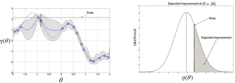
Figure 1: The expected improvement heuristic. The heuristic assesses the value of observing new points. On the left we consider the point circled (in black) atθ=−.86. On the right we illustrate the expected improvement assuming thatP(η(θ)|θ=−.86) is Gaussian. To be considered an improvement the value ofη(θ) must exceed the value of the current maximumf max. The probability mass associated with the expected improvement is shaded. The expected improvement is proportional to the expected value of the indicated mass.
3.2 Objective Function Model
As a Bayesian method the performance of BO depends profoundly on the quality of the modeling effort. The specification of the prior distribution determines the nature of the posterior and hence the generalization performance of the surrogate representation. We elect to model the objective function using a Gaussian process (Rasmussen and Williams, 2005),
η(θ)∼GP(m(θ), k(θ, θ0)).
GP models are defined by a mean function m(θ) and a covariance function k(θ, θ0). The mean function specifies the expected value at a given point m(θ) =E[η(θ)]. Likewise, the covariance function estimates the covariancek(θ, θ0) =E[(η(θ)−m(θ))(η(θ0)−m(θ0))] The kernel function encodes how correlated values of the objective are at points θand θ0. Both of these functions encode knowledge of the underlying class of functions.
For the purpose of computing the improvement function described above, the posterior distribution at new points must be computed. In the GP model, this posterior has a simple form. Given the data D1:n the conditional posterior distribution is Gaussian with mean,
µ(η(θn+1)|D1:n) =m(θn+1)−k(θn+1, θ)K(θ, θ)−1(y−m), wheremis a vector of size n with elementsm(θ1), ..., m(θn) and variance,
σ2(η(θn+1)|D1:n) =k(θn+1, θn+1)−k(θn+1, θ)tK(θ, θ)−1k(θ, θn+1).
Define y to be the column vector of observed performances such that yi = η(θi). Define
Algorithm 1 Bayesian Optimization Algorithm (BOA) 1: LetD1:n={(θi,ηˆ(θi), ξi)}|ni=1.
2: repeat
3: Compute the matrix of covariancesK.
4: Select the next policy to evaluate: θn+1= arg maxθEP(η(θ)|D)[I(θ)].
5: Execute the policyθn+1 for E episodes.
6: Compute Monte-Carlo estimate of expected return ˆη(θn+1) =E1 Pξ∈ξn+1R¯(ξ)
7: UpdateD1:n+1=D1:n∪(θn+1,ηˆ(θn+1))
8: untilConvergence
the column vector of correlations such that theith element is k(θn+1, θi) (k(θn+1, θ)t is the transpose of this vector).
3.3 Bayesian Optimization for RL
Algorithm 1 outlines the basic loop of the BO routine discussed above. Line 1 assumes a batch of data of the form,D1:n={(θi, η(θi), ξi)}|ni=1. Hereafter, we will writeDto indicate the collection of ndata tuples. The Monte-Carlo estimate for policy θi is computed using
a set of trajectories ξi sampled from the target system. Given data D, the surface of the
expected return is modeled using the GP. The kernel matrix K is pre-computed in line 3 for reuse during maximization of the EI. Line 4 maximizes the EI. For this purpose, any appropriate optimization package can be used. To compute the expected improvement the GP posterior distribution P(η(θn+1|D)) must be computed. This entails computing the mean function m(θn+1), the vector of covariances k(θn+1, θ), and performing the required multiplications. Additional computational costs introduced into the mean and kernel func-tions will impact the computational cost of the optimization. Our modificafunc-tions to the underlying model will increase these costs, but lead to more efficient search of the objective function space. The additional costs must be balanced against the cost of evaluating the objective function. Once selection is completed, new trajectories are generated from the selected policy (line 5), and an estimate of the expected return is recorded (lines 6 and 7).
4. Incorporating Trajectory Information into Bayesian Optimization for RL
4.1 Model-Free RL via Bayesian Optimization: A Behavior-Based Kernel (BBK)
In this section we design a kernel for the RL setting that leverages trajectory data to com-pute a domain independent measure of policy relatedness. Consider BO algorithms as a kind of space filling algorithm. Wherever sufficient uncertainty exists, the algorithm will aim to select a point to fill that space thereby reducing uncertainty in the vicinity of the selected point. The kernel function defines the volume to be filled. It is important for the development of BO algorithms for RL that kernel functions are robust to the parametriza-tion of the policy space. Most kernel funcparametriza-tions do not have this property. For instance, squared exponential kernels require that policies have a finite and fixed number of param-eters. The kernel cannot compare non-parametric policies. In this case, individual policies can have distinct structures preventing their comparison using this form of kernel function. We seek a kernel function which is useful for comparing policies with distinct structural forms.
To construct an appropriate representation of uncertainty for the RL problem we propose relating policies by their behaviors. We define the behavior of a policy to be the associated trajectory densityP(ξ|θ). Below, we discuss how to use the definition to construct a kernel function and how to estimate the kernel values without learning transition and reward functions.
To develop our kernel and demonstrate its relationship to the expected return we prove the following theorem:
Theorem 1 For anyθi, and θj, Rmax≥0
|η(θi)−η(θj)| ≤Rmax
√
2pKL(P(ξ|θi)||P(ξ|θj)) +
p
KL(P(ξ|θj)||P(ξ|θi))
.
Proof: Below we establish the upper bound stated above. To begin we rewrite the absolute value of the difference in expected returns,
|η(θi)−η(θj)|=
Z ¯
R(ξ)P(ξ|θi)dξ−
Z
¯
R(ξ)P(ξ|θj)dξ
= Z ¯
R(ξ)(P(ξ|θi)−P(ξ|θj))dξ
.
By moving the absolute value into the integrand we upper bound the difference,
Z ¯
R(ξ)(P(ξ|θi)−P(ξ|θj))dξ
≤ Z
|R¯(ξ)(P(ξ|θi)−P(ξ|θj))|dξ.
We define a new quantityRmaxbounding the trajectory reward from above. The trajectory reward is simply the sum of rewards at each trajectory step. Rmax is defined to be the maximal trajectory value. Using theRmaxquantity we construct a new bound,
Z
|R¯(ξ)(P(ξ|θi)−P(ξ|θj))|dξ≤Rmax
Z
|P(ξ|θi)−P(ξ|θj)|dξ,
1
2(V(P, Q))
2 ≤ KL(P||Q) where V is the variational distance, R
|(P(x)−Q(x))|dx, and
KL(P, Q) is the Kullback Leibler divergence,
KL(P(ξ|θi)||P(ξ|θj)) =
Z
P(ξ|θi) log
P(ξ|θi)
P(ξ|θj)
dξ.
We can use Pinsker’s inequality to upper bound the variational distance,
Rmax
Z
|P(ξ|θi)−P(ξ|θj)|dξ≤Rmax
√
2
q
KL(P(ξ|θi)||P(ξ|θj)).
Finally, we use the fact that the variational distance is symmetric R
|(P(x)−Q(x))|dx=
R
|(Q(x)−P(x))|,
|η(θi)−η(θj)| ≤ Rmax
√
2
q
KL(P(ξ|θi)||P(ξ|θj))
≤ Rmax
√
2
hq
KL(P(ξ|θi)||P(ξ|θj)) +
q
KL(P(ξ|θj)||P(ξ|θi))
i
.
Hence, this simple bound relates the difference in returns of two policies to the trajectory density.
Importantly, the bound is a symmetric positive measure of the distance between poli-cies. It bounds, from above, the absolute difference in expected value, and reaches zero only when the divergence is zero (the policies are the same). Additionally, computing the tighter variational bound,Rmax R
|P(ξ|θi)−P(ξ|θj)|dξ, inherently requires knowledge of
the domain transition models. Alternatively, the log term of the KL-divergence is a ratio of path probabilities. Given a sample of trajectories the ratio can be computed with no knowledge of the domain model. This characteristic is important when learned transition and reward functions are not available. Our goal is to incorporate the final measure of pol-icy relatedness into the surrogate representation of the expected return. Unfortunately, the divergence function does not meet the standard requirements for a kernel (Moreno et al., 2004). To transform the bound into a valid kernel we first define a function,
D(θi, θj) =
q
KL(P(ξ|θi)||P(ξ|θj)) +
q
KL(P(ξ|θj)||P(ξ|θi)),
and define the covariance function to be the negative exponential of D,
K(θi, θj) = exp(−α·D(θi, θj)).
The kernel has a single scalar parameter α controlling its width. This is precisely what we sought, a measure of policy similarity which depends on the action selection decisions. The kernel compares behaviors rather than parameters, making the measure robust to changes in policy parameterization.
4.2 Estimation of the Kernel Function Values
Below we discuss using estimates of the divergence values in place of the exact values for
D(θi, θj). Computing the exact KL-divergence requires access to a model of the decision
The divergence must be estimated. In this work we elect to use a simple Monte-Carlo estimate of the divergence. The divergence between policy θi and θj is approximated by,
ˆ
D(θi, θj) =
X
ξ∈ξi
log
P(ξ|θi)
P(ξ|θj)
+X
ξ∈ξj
log
P(ξ|θj)
P(ξ|θi)
,
using a sparse sample of trajectories generated by each policy respectively (ξi represents
the set of trajectories generated by policy θi). Because of the definition of the trajectory
density, the term within the logarithm reduces to a ratio of action selection probabilities,
log
P(ξ|θ
i) P(ξ|θj)
= log P0(s0) QT
t=1P(st|st−1, at−1)Pπ(at−1|φ(st−1), θi) P0(s0)Q
T
t=1P(st|st−1, at−1)Pπ(at−1|φ(st−1), θj)
! = T X t=1 log P
π(at|st, θi) Pπ(at|st, θj)
,
and is easily estimated using trajectory data.
A problem arises when computing the Expected Improvement (Line 4 of the BOA). Computing the conditional mean and covariance for new points requires the evaluation of the kernel for policies which have no trajectories present in the data set. We elect to use an importance sampled estimate of the divergence, because we do not have access to learned transition and reward functions,
ˆ
D(θnew, θj) =
X
ξ∈ξj
P(ξ|θnew) P(ξ|θj)
log P(ξ
|θnew) P(ξ|θj)
+ log
P(ξ
|θj) P(ξ|θnew)
.
Though the variance of this estimate can be large, our empirical results show that errors in the divergence estimates, including the importance sampled estimates, do not negatively impact performance. Alternative methods of estimating f-divergences (KL-divergence being a specific case) have been proposed in the literature (Nguyen et al., 2007), and can be used for future implementations.
4.3 Model-Based RL via Bayesian Optimization
The behavior based kernel has some important limitations. First, due to the definition of the BBK the kernel can only compare stochastic policies. The KL divergence is meaningful when the conditional trajectory densities share the same support. Second, the upper bound used to construct the kernel function is loose. This can lead to excessive exploration when the kernel exaggerates the differences between policies. In this section, we introduce a distinct method of leveraging trajectory data that does not require stochastic policies and can leverage any appropriate kernel function (including the BBK).
trajectories are sampled from the approximate trajectory density,
ˆ
P(ξ|θ) = ˆP0(s0)
T
Y
t=1 ˆ
P(st|st−1, at−1)Pπ(at−1|φ(st−1), θ).
We write ˆP to indicate that the transition function and initial state distribution have been learned from the observed trajectory data. From a fixed sample ofE simulated trajectories we compute a model-based Monte-Carlo estimate of the expected return,
m(θ, D) = ˆη(θi) =
1
E
E
X
j=1 ˆ
R(ξj).
The function ˆR indicates the learned reward function.
If the agent has learned accurate domain models an optimal policy can be learned by maximizingθ∗= arg maxθm(θ, D). Unfortunately, in many domains it is difficult to specify
and to learn accurate domain models. In the worst case, the domain model classes selected by the designer may not contain the true domain models. Moreover, the cost of sampling trajectories may become prohibitive as the complexity of the domain models increases. Therefore, we wish to allow the designer the flexibility of selecting a class of domain models that is simple, efficient, and possibly an inaccurate representation of the target system. In our work we propose a means of accurately estimating the expected return despite domain model errors.
To overcome problems stemming from the predictive errors we propose usingm(θ, D) as the prior mean function for the GP model thereby modeling the deviations from this mean as a GP. The predictive distribution of the GP changes to be Gaussian with mean,
µ(η(θn+1)|D) =m(θn+1, D) +kt(θn+1, θ)K(θ, θ)−1(η−m(θ, D)),
wherem(θ, D) = (m(θ1, D), ..., m(θn, D)) is a column vector of Monte-Carlo estimates with
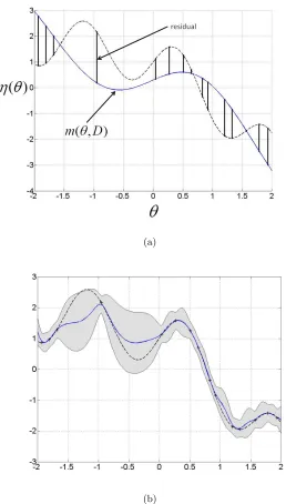
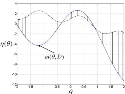
an element for each policy in D (This vector must be recomputed when new trajectories are added to the data). The variance remains unchanged. The new predictive mean is a sum of the Monte-Carlo approximation of the expected return and the GP’s prediction of the residual. We illustrate the advantage of this model in Figure 3. As shown in the figure the model of the residuals directly compensates for errors introduced by the learned domain models.
In the case where the domain models cannot be effectively approximated, the model-based estimates of the expected return may badly skew the predictions. Consider the following degenerate case: m(θ, D1:n) underestimates the true mean for all policies resulting
in zero expected improvement in the region of the optimal policy. In this case, the pessimistic estimates stifle the exploration of the policy space thereby preventing the discovery of the optimal solution. Our goal is to account for the domain model bias in a principled way.
We propose a new model of the expected return,
η(θ) = (1−β)η1(θ) +βη2(θ).
(a)
(b)
functionη2(θ)∼GP(m(θ, D1:n), k(θ, θ)) with a GP distribution that uses the model-based
mean m(θ, D) introduced above. The kernel of both GP priors is identical. The resulting distribution for η(θ) ∼ GP(βm(θ, D), c(β)k(θ, θ)) is a GP with prior mean βm(θ, D) and covariance computed using the kernel function. This change impacts the predicted mean which now weights the model estimate byβ,
µ(θn+1|D) =βm(θn+1, D) +k(θn+1, θ)K(θ, θ)−1(η(θ)−βm(θ, D)). The variance changes to incorporate a factor c(β).
We choose to optimize the β parameter using evidence maximization (Rasmussen and Williams, 2005). For a GP with mean βm and covariance matrix K the log likelihood of the data is,
P(η(θ)|D) =−1
2(η(θ)−βm(θ, D))
tK−1(η(θ)−βm(θ, D))−1
2log|K| −
n
2 log(2π). Taking the gradient of the log likelihood and solving forβ results in a closed form solution,
β = η(θ)
tK−1m(θ, D)) m(θ, D))tK−1m(θ, D)).
Optimizing the value ofβ, prior to maximizing the expected improvement, allows the model to control the impact of the mean function on the predictions. This tradeoff is illustrated in Figure 4. Intuitively, the algorithm can return to the performance of the unmodified BOA when the domain models are poor (by setting β to zero).
Algorithm 2 outlines the steps necessary to incorporate the new model into the BOA. MBOA takes advantage of trajectory data by building an approximate simulator of the expected return. Like the BBK the prior mean function used by the MBOA only requires policies to output actions. It is oblivious to the internal structure of policies. Additionally, by contrast to the BBK, MBOA can compare stochastic and deterministic policies.
Most work in model-based RL assumes the learned transition and reward functions are unbiased estimators of the true functions. This is difficult to guarantee in real-world tasks. Due to our limited knowledge transition and reward models frequently exhibit considerable model bias. MBOA aims to overcome sources of bias by combining a weighted mean function with a residual model. By construction MBOA can ignore the mean function if it produces systematic errors, due to model bias, and can benefit from the mean function where the estimates are accurate. In the results section we provide examples where MBOA benefits from the use of simple (biased) transition and reward models.
5. Experiment Results
(a) An illustration of the degenerate case where the mean function systematically under-estimates the objective function (objective function marked by dashed line).
(b) The corrected model with control parameter β = 1. After correction the model un-derestimates the objective function.
(c) The corrected model with control parameterβ =.1. By reducing the influence of the mean function the model more accurately estimates the true function.
Algorithm 2 Model-based Bayesian Optimization Algorithm (MBOA) 1: LetD1:n={θi, η(θi), ξ}|ni=1.
2: repeat
3: Learn the transition function, reward function, and initial state distribution from trajectory data.
4: Compute the vectorm(θ, D1:n) using the approximate simulator.
5: Optimizeβ by maximizing the log likelihood.
6: Select the next point in the policy space to evaluate: θn+1= arg maxθE(I(θ)|D1:n).
7: Execute the policy with parametersθn+1 in the MDP.
8: UpdateD1:n+1=D1:n∪(θn+1, η(θn+1), ξn+1)
9: untilConvergence.
5.1 Experiment Setup
We detail the special requirements necessary to implement each algorithm in this section. For all experiments, except Cart-pole, the policy search algorithms search for parametric soft-max action selection policies,
P(a|s) = Pexp(θa·f(s))
y∈Aexp(θy·f(s))
.
The parametersθy are the set of policy parameters associated with actiony. The function
f(s) computes features of the state.
In the Cart-pole experiments, a linear policy maps directly to the action,
a=θ·f(s) +.
Epsilon is a small noise parameter used in algorithms requiring stochastic policies. Below we discuss the implementations of each algorithm.
• MBOA and BOA. The GP model used in MBOA and BOA can accept any kernel function (including the BBK). Below we show results comparing these kernels. Unless stated otherwise the squared exponential kernel,
k(θi, θj) = exp(−
1
2ρ(θi−θj)
t(θ
i−θj)),
is used in our experiments. The width of this kernel is controlled by the scaling parameter ρ. The ρ parameter was tuned for each experiment, and the same value was used in both MBOA and BOA. The prior mean function of BOA is the zero function, and MBOA employs the model-based mean function discussed above.
bounds on the policy parameters. We specify an upper bound of 1 and a lower bound of -1 for each dimension of the policy. These bounds hold for all experiments reported below.
To implement the MBOA the designer must define a class of domain models. For the experiments reported below linear models were used. The models are of the form,
sti =wi·φ(st−1, at−1)
t, rt=w
r·φ(st−1, at−1, st)0,
where st,i is theith state variable at time t, wi is the weight vector for the ith state
variable, andφ(st−1, at−1, st)0is a column vector of features computed from the states and actions (and next states in the case of the reward model). The features used in our experiments are found in Table 1. Parameterswi andwrare estimated from data
using standard linear regression.
• PILCO. We use an implementation of PILCO provided by the authors Deisenroth and Rasmussen (2011). This implementation uses sparse GPs to learn the transition and reward functions of the MDP.
• DYNA-Q. We make two slight modifications to the DYNA-Q algorithm. First, we provide the algorithm with the same linear models employed by MBOA. These are models of continuous transition functions which DYNA-Q is not normally suited to handle. The problem arises during the sampling of previously visited states during internal reasoning. To perform this sampling we maintain a dictionary of past observa-tions and sample visited states from it. These continuous states are discretized using a CMAC function approximator. The second change we make is to disallow inter-nal reasoning until a trial is completed. To reduce the computatiointer-nal cost reasoning between steps is not allowed. After each trial DYNA-Q is allowed 200000 internal samples to update its Q-function. This was to ensure that during policy selection DYNA-Q was allowed computational resources comparable to the resources used by MBOA and BOA with the BBK.
• Q-Learning with CMAC function approximation. -Greedy exploration is used in the experiments ( is annealed after each step). The discretization of the CMAC approximator was chosen to give robust convergence to good solutions.
• OLPOMDPOLPOMDP is a simple gradient based policy search algorithm (Baxter et al., 2001). The OLPOMDP implementations use the same policy space optimized by the BO algorithms.
Domain/Features Transition Function Reward Function Policy Description Mountain Car quadratic expansion:
(l, u, cos(l), cos(u), action)
quadratic expansion: (l, u, cos(l), cos(u), action)
cubic expansion: l, u
Variable l denotes the location and u denotes the velocity of the car.
Acrobot quadratic expansion: (θ1, θ2,θ˙1,θ˙2, action)
quadratic expansion: (θ1, θ2,θ˙1,θ˙2, cos(θ1), cos(θ2), action)
(θ1, θ2,θ˙1,θ˙2) (θ1, θ2) are the angles between the
links and ( ˙θ1,θ˙2) are the angular
velocities. Cart Pole (v,v, ω,˙ ω, action,˙
sin(ω), cos(ω), sin(ω), 1/cos(ω))
(v,v, ω,˙ ω, action,˙ sin(ω), cos(ω), sin(ω), 1/cos(ω), v >4, v < −4, ω >π4, ω <−π
4)
(v, v0, ω,ω˙) (v, v0) is the velocity and change in velocity of the cart, (ω, ω0), is the angle of the pole, and angular ve-locity of the pole.
3-link Planar Arm (θ1, θ2, θ3, xt, yt, action)
(θ1, θ2, θ3,(xt−xg)2, (yt−yg)2, action)
(xt−xg, yt−yg) (θ1, θ2, θ3) are the link angles,
(xt, yt) is the location of the arm tip, and (xg, yg) is the goal loca-tion.
Bicycle (ω,ω, ν,˙ ν, x˙ f, xr, yf,
yr, action)
(ω,ω, ν,˙ ν, x˙ f, xr, yf,
yr, action,|ω|>15π))
See Lagoudakis et al. (2003) for policy features.
Variables (xf, xr, yf, yr) represent the locations of the front and rear tires respectively.
Table 1: Features for the transition function, reward function, and policy function.
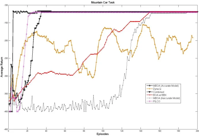
Figure 5: Mountain Car Task: We report the total return per episode averaged over 40 runs of each algorithm.
5.2 Mountain Car Task
The sparse reward signal makes Mountain Car an ideal experiment for illustrating the importance of directed exploration based on differences in policy behavior. Approaches based on random exploration and exploration weighted by returns are poorly suited to this kind of domain (we have excluded the other model-free methods from the graph because they fail to improve within 200 episodes). Visual inspection of the performance of BOA shows that many of the selected policies, which are unrelated according to the squared exponential kernel, produce similar action sequences when started from the initial state. This redundant search is completely avoided when generalization is controlled by the BBK. Note that the performance of all kernel methods depends on the settings of the pa-rameters. Optimization of the hyper parameters is not the focus of this work. However, the parameters of the BBK (and any other kernel used with MBOA) can be automati-cally optimized using any standard method of model selection for GP models (Rasmussen and Williams, 2005). We elect to simply set the parameter of the BBK, α, to 1 for all experiments.
When accurate domain models can be learned, the Monte-Carlo estimates of the ex-pected return computed by the MBOA will accurately reflect the true objective. Therefore, if the domain models can be accurately estimated with few data points MBOA will rapidly identify the optimal policy. To illustrate this we hand-constructed a set of features for the linear domain models used in the mountain car task. Depicted in Figure 5 are the results for MBOA with high quality hand-constructed features. Once the domain models are es-timated, only four episodes are needed to yield accurate domain models. Once accurate domain models are available MBOA immediately finds an optimal policy. Typically, the in-sight used to construct model features is not available in complex domains. To understand the performance of MBOA in settings with poor insight into the correct domain model class, we remove the hand constructed features from the linear models and examine the resulting performance. With poor models, the performance of the MBOA degrades. As shown in the figure, the performance of MBOA is no longer better than the performance of standard BOA with the model-free BBK. The BBK can be combined with the model-based mean function used in MBOA. We show the performance of this combination, using the BBK as the kernel function for the MBOA, labeled Combined, in Figure 5. The results are comparable to the case where MBOA has access to high quality domain models. The performance of PILCO is comparable to the combined algorithm. After 20 episodes the PILCO algorithm has identified a high quality policy for the task. However, PILCO uses all available transition data to train the sparse GP models of the transition and reward function. After 30 episodes the kernel matrices consume all available memory and force the algorithm to page to disk. Due to this problem we terminated the PILCO experiments after 30 episodes, and we report the value of the optimal policy found by PILCO after this point. By contrast, the cost of GP prediction for MBOA grows with the number of episodes, and MBOA exploits a less complex (linear) class of domain models. Consequently, it discovers the optimal policy using less experience and less computational resources.
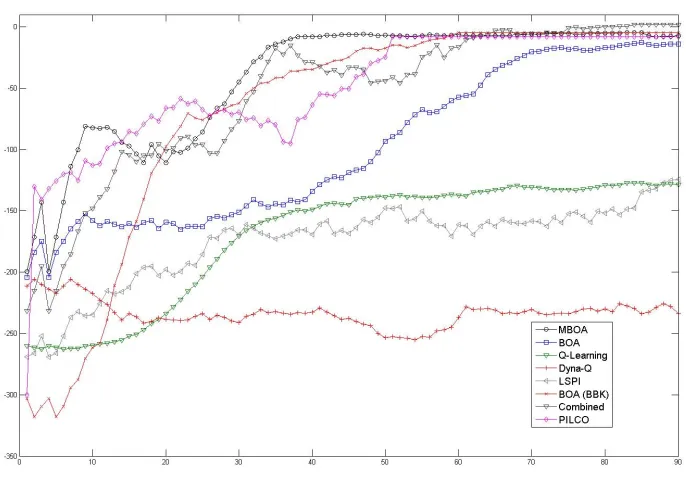
Figure 6: Acrobot Task: We report the total return per episode averaged over 40 runs of each algorithm.
still identify the optimal policy. Standard model-based RL algorithms, such as DYNA-Q, cannot learn optimal policies when confronted with systematic domain model errors.
5.3 Acrobot Task
In the acrobot domain, the goal is to swing the foot of the acrobot over a specified threshold by applying torque at the hip. Details of the implementation can be found in Sutton and Barto (1998). Four features are used for the soft-max policy resulting in twelve policy parameters. The acrobot results are shown in Figure 6.
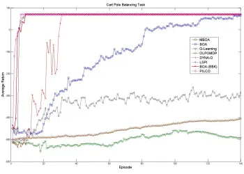
Figure 7: Cart Pole Task: We report the total return per episode averaged over 40 runs of each algorithm.
PILCO results after 50 episodes. Thereafter we report the performance of the best policy found by PILCO.
5.4 Cart-pole Task
In the Cart-pole domain, the agent attempts to balance a pole fixed to a movable cart. The policy selects the magnitude of the change in velocity (positive or negative) applied to the base of the cart. The policy is a function of four features (v, v0, ω, ω0), the velocity, change in velocity, angle of the pole, and angular velocity of the pole. The reward function gives a positive reward for each successful step. A penalty is added to this reward when pole angles deviate from vertical, and when the location of the cart deviates from the center. A large positive reward is received after 1000 steps if the pole has been kept upright and the cart has remained within a fixed boundary. Episodes terminate early if the pole falls or the cart leaves its specified boundary.
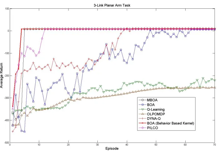
Figure 8: Planar Arm Task: We report the total return per episode averaged over 40 runs of each algorithm.
episodes before similar performance is achieved. LSPI converges faster but cannot match the performance of either the BOA or MBOA. Please note that our problem is distinct from the original LSPI balancing task in the following ways: 1. The force applied by the agent is more restricted. 2. The cart is constrained to move within a fixed boundary. 3. The reward function penalizes unstable policies. After 30 episodes the DYNA-Q algorithm has found a solution comparable to that of MBOA. This performance is unsurprising given the accuracy of the estimated domain models. PILCO learns a high quality model given two episodes of experience and finds an optimal policy by the third episode. In the cart-pole task learning a local model around the balance point is sufficient to perform well and this contributes to PILCO’s exceptional performance.
5.5 3-Link Planar Arm Domain
The performance of each algorithm is shown in Figure 8. The generalization of the divergence-based kernel, BOA(BBK), is particularly powerful in this case. Much of the policy space is quickly identified to be redundant and is excluded from the search. The agent fixes on an optimal policy almost immediately. Like the Cart-pole task, the transition and reward function of the arm task are linear functions. Once the functions are estimated MBOA quickly identifies the optimal policy (the mean function accurately reflects the true surface). Additional data is needed before the BOA identifies policies with similar quality. The other model-free alternatives require 1000 episodes before converging to the same result. DYNA-Q found a policy comparable to the MBOA, but required more experience. In the three tasks discussed above the MBOA makes better use of the available computational resources and remains robust to model bias. PILCO very quickly finds an optimal policy in this task. After ten episodes PILCO has learned an accurate GP model of the transition dynamics. Thereafter, PILCO finds a near optimal policy. We have extrapolated PILCO’s performance beyond the 20th episode. Each PILCO run required 3 weeks to generate the first 20 episodes.
5.6 Bicycle Balancing
Agents in the bicycle balancing task must keep the bicycle balanced for ten minutes of simulated time. For our experiments we use the simulator originally introduced in Randlov and Alstrom (1998). The state of the bicycle is defined by four variables (ω,ω, ν,˙ ν˙). The variableω is the angle of the bicycle with respect to vertical, and ˙ω is its angular velocity. The variableν is the angle of the handlebars with respect to neutral, and ˙ν is the angular velocity. The goal of the agent is to keep the bicycle from falling. Falling occurs when
|ω| > π/15. The same discrete action set used in Lagoudakis et al. (2003) is used in our implementations. Actions have two components. The first component is the torque applied to the handlebars T ∈ (−1,0,1), and the second component is the displacement of the rider in the saddle p ∈ (−.02,0, .02). Five actions are composed from these values (T, p) ∈ ((−1,0),(1,0),(0,−.02),(0, .02),(0,0)). The reward function is defined to be the squared change inω, (ωt−ωt+1)2, at each time step. An additional -10 penalty is imposed if the bicycle falls before time expires. Rewards are discounted in time insuring that longer runs result in smaller penalties. In our implementation the set of 20 features introduced in Lagoudakis et al. (2003) were used. The softmax policy has 100 parameters. Please note that our LSPI implementation of bicycle does not benefit from the design decisions introduced in Lagoudakis et al. (2003).
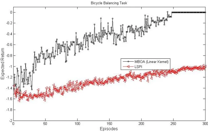
Figure 9: Bicycle Balancing Task: We report the total return per episode averaged over multiple runs of each algorithm (15 runs of MBOA and 30 runs of LSPI).
likelihood after each policy execution. Before optimization of the hyper-parameters the algorithm was made to choose 20 policies with the uninformed values. MBOA uses very simple and highly inaccurate linear models in this task. Errors in the linear models are significant enough to cause DYNA-Q to fail. MBOA exhibits robust performance despite the predictive errors caused by model bias. It converges to a near optimal policy and exhibits excellent data efficiency.
We allowed the PILCO algorithm to run for three weeks. After this period each run had completed only 24 episodes. This was due to the size of the kernel covariance matri-ces. Taken together these matrices consumed several gigabytes of memory and forced the algorithm to access the hard disk. This is a serious problem with using (sparse) GP mod-els to represent the transition and reward function in MDPs. Unfortunately, the PILCO algorithm had not found a high quality policy given the available experience. We elected to exclude these results from the depicted experiments.
6. Related Work
Gaussian processes have been used to model functions of interest in the RL setting. Related work employing Gaussian processes in RL includes Engel et al. (2003, 2005) in which the value function is modeled as a Gaussian Process, Ghavamzadeh and Engel (2007a,b) wherein GPs were used to model the gradient of the expected return, and the work of Deisenroth and Rasmussen (2011) and Rasmussen and Kuss (2004) where GPs were used to model the transition and reward functions.
Work by Engel et al. (2003, 2005) focuses on the problem of estimating the value function given a fixed action selection policy. GP models are used to approximate the value function; The GP model introduces a smoothness prior on the space of value functions. Similarly, Ghavamzadeh and Engel (2007a,b) focus on the problem of estimating the gradient of the value function for a fixed action selection policy. It should be noted that the kernel described by Ghavamzadeh and Engel (2007b) exploit trajectory information; the authors propose a Fisher kernel for relating sampled trajectories. This facilitates generalization across sampled trajectories and leads to improved estimates of the gradient of the value function. The results of their experiments show consistent improvement, in a set of benchmark problems, over standard Monte-Carlo methods for estimating the gradient of the expected return. However, their kernel cannot be used to compare policies as is done in our work. During the process of policy improvement their approach re-samples trajectory data for each new policy. In contrast, the GP models discussed in this article perform off-policy estimation of the expected return and re-use sampled trajectory data to approximate the returns of new policies.
Numerous model-based Bayesian RL algorithms exploit Bayesian priors on the domain model parameters (Dearden et al., 1999; Strens, 2000; Duff, 2003; Deisenroth and Ras-mussen, 2011; Rasmussen and Kuss, 2004). The priors encode the agents uncertainty of the world it lives within. Like our algorithm, these methods actively explore to reduce uncer-tainty. For instance, work by Dearden et al. (1999) introduced a method for representing Bayesian belief states and proposed an action selection policy based on Value of Information (this policy was first introduced in Dearden et al. 1998). Related work by Strens (2000) and Duff (2003) introduced new approaches for approximately solving the Bayesian belief state MDP. An approximate solution of the belief state MDP can be used to derive an action selection policy that approximates Bayes optimal action selection. Our work explores the problem of Bayesian parametric policy search and exploits a heuristic for directed explo-ration of the parametric policy space. However, we avoid Bayesian modeling of the domain models. Instead, our approach directly represents uncertainty of the expected return. Our empirical results demonstrate how this impacts practical application.
To understand the consequences of this decision consider the recent work by Deisenroth and Rasmussen (2011) whom developed the PILCO algorithm. PILCO learns GP models of the transition and reward functions. The learned transition and reward functions are used to approximate the expected return via prediction of state-reward sequences. The policy is optimized by analytic gradient ascent on the approximated expected return. To represent a GP model of the transition and reward function it is necessary to represent a matrix with
exploding in size. For instance, in the experiments above our kernel matrices include at most 3002 elements whereas PILCO’s kernel matrices quickly explode to more than 400002 elements. Sparse GP inference can help to reduce the costs of dealing with these large matrices. However, as is demonstrated in our experiments we found that sparse inference was not sufficient to overcome the performance problems. The advantage of the approach can be further improved by introducing heuristic local search techniques for discovering the maximum of the expected improvement function.
Work by Kakade (2001) presented a metric based on the Fisher information to derive the natural policy gradient update. Kakade (2001) demonstrated that natural policy gradient methods outperform standard gradient methods in a difficult Tetris domain. Follow up work by Bagnell and Schneider (2003) proposed pursuing a related idea within the path integral framework for RL (the same framework of this paper). Their work considered metrics defined as functions on the distribution over trajectories generated by a fixed policy
P(ξ|θ). In contrast to our goals both works focus on iteratively improving a policy via gradient descent. Furthermore, no explicit attention is paid to using the metric information to guide the exploratory process. However, the insight that policy relationships should be expressed as functions of the trajectory density has played a key role in the development of our behavior based kernel.
Work by Peters et al. (2010) and Kober and Peters (2010) is related to our proposed kernel function. Peters et al. (2010) used a divergence-based bound to control exploration. Specifically, they attempt to maximize the expected reward subject to a bound proportional to the KL-divergence between the empirically observed state-action distribution and the state-action distribution of the new policy. The search for a new policy is necessarily local, restricted by the bound to be close to the current policy. By contrast, our work uses the divergence as a measure of similarity and performs a global, aggressive, search of the policy space. Work by Kober and Peters (2010) derives a lower bound on the importance sampled estimate of the expected return, as was done in Dayan and Hinton (1997), and observes the relationship to the KL-divergence of the reward weighted behavior policy and the target policy. They derive from this relationship an EM-based update for the policy parameters. An explicit effort is made to construct the update such that exploration is accounted for. However, their method of state-dependent exploration is based on random perturbations of the action selection policy. Our method of exploration is instead determined by the posterior uncertainty and does not depend on a behavior policy.
7. Conclusions
General black box Bayesian optimization algorithms have been adapted to the RL policy search problem, and have shown promise in difficult domains. We show how to improve these algorithms by exploiting trajectory data generated by agents.
For model-free RL, we presented a new kernel function for GP models of the expected return. The kernel compares sequences of action selection decisions from pairs of policies. We motivated our kernel by examining a simple upper bound on the absolute difference of expected returns for two arbitrary policies. We used this upper bound as the basis for our kernel function, argued that the properties of the bound ensure a more reasonable measure of policy relatedness, and demonstrated empirically that this kernel can substantially speed up exploration. The empirical results show that the derived kernel is competitive with the model-based RL algorithms MBOA and Dyna-Q, and converge more quickly than the model-free algorithms tested. Additionally, we showed that in certain circumstances BBK can be combined with the MBOA to improve the quality of exploration.
For model-based RL we presented MBOA for model-based RL. MBOA improves on the standard BOA algorithm by using collections of trajectories to learn an approximate simulator of the decision process. The simulator is used to define an approximation of the underlying objective function. Potentially, such a function provides useful information about the performance of unseen policies which are distant (according to a measure of similarity) from previous data points. Empirically, we show that the MBOA has exceptional data efficiency. Its performance exceeds LSPI, OLPOMDP, Q-Learning with CMAC function approximation, BOA, and DYNA-Q in all but one of our tasks. MBOA performs well even when the learned domain models have serious errors. Overall, MBOA appears to be a useful step toward combining model-based methods with Bayesian optimization for the purposes of handling approximate models and improving data efficiency.
The penalty for taking this approach is straightforward. A substantial increase in com-putational cost is incurred during optimization of the surrogate function. This occurs when evaluating MBOA’s approximate simulator, or when estimating the values of the behavior based kernel. In both cases the cost of evaluating the kernel function grows linearly in the length of the trajectories. However, the cost is compounded during optimization and will make these approaches infeasible when trajectory lengths become huge. Overcoming this barrier is an important step towards taking advantage of trajectory data generated in complex domains.
Acknowledgments
We gratefully acknowledge the support of the Office of Naval Research under grant number N00014-11-1-0106, the Army Research Office under grant number W911NF-09-1-0153, and the National Science Foundation under grant number IIS-0905678.
References
San Francisco, CA, USA, 2003.
J. Baxter, P. Bartlett, and L. Weaver. Experiments with infinite-horizon, policy-gradient estimation. Journal of Artificial Intelligence Research, 15(1):351–381, 2001.
M. Belkin and P. Niyogi. Using manifold structure for partially labelled classification. In
Advances in Neural Information Processing Systems, pages 929–937, Vancouver, B.C., CA, 2002.
E. Brochu, V. Cora, and N. de Freitas. A tutorial on Bayesian optimization of expensive cost functions, with application to active user modeling and hierarchical reinforcement learning. Technical Report TR-2009-023, 2009.
P. Dayan and G. Hinton. Using expectation-maximization for reinforcement learning.Neural Computation, 9:271–278, 1997.
R. Dearden, N. Friedman, and S. Russell. Bayesian q-learning. In Proceedings of the Fifteenth National Conference on Artificial Intelligence, pages 761–768, 1998.
R. Dearden, N. Friedman, and D. Andre. Model-based bayesian exploration. InUncertainty in Artificial Intelligence, pages 150–159, Stockholm, Sweden, 1999.
M. Deisenroth and C. Rasmussen. PILCO: A model-based and data-efficient approach to policy search. In Proceedings of the Twenty-Eigth International Conference on Machine Learning, pages 465–472, Bellevue, Washington, USA, 2011.
M. Duff. Design for an optimal probe. In Proceedings of the Twentieth International Conference on Machine Learning, pages 131–138, Washington, DC, USA, 2003.
Y. Engel, S. Mannor, and R. Meir. Bayes meets bellman:the Gaussian process approach to temporal difference learning. In Proceedings of the Twentieth International Conference on Machine Learning, pages 154–161, Washington, DC, USA, 2003.
Y. Engel, S. Mannor, and R. Meir. Reinforcement learning with Gaussian processes. In
Proceedings of the Twenty-Second International Conference on Machine Learning, pages 201–208, University of Bonn, Germany, 2005.
M. Ghavamzadeh and Y. Engel. Bayesian actor-critic algorithms. In Proceedings of the Twenty-Fourth International Conference on Machine Learning, pages 297–304, Oregon State University, Corvallis, USA, 2007a.
M. Ghavamzadeh and Y. Engel. Bayesian policy gradient algorithms. InProceedings of the Twentieth Annual Conference on Neural Information Processing Systems, pages 457–464, Vancouver, B.C., CA, 2007b.
N. Hansen. The CMA evolution strategy: A comparing review. In J.A. Lozano, P. Lar-ranaga, I. Inza, and E. Bengoetxea, editors, Towards a New Evolutionary Computation. Advances on Estimation of Distribution Algorithms, pages 75–102. Springer, 2006.
S. Kakade. A natural policy gradient. In Advances in Neural Information Processing Systems, pages 1531–1538, Vancouver, B.C., CA, 2001.
J. Kober and J. Peters. Policy search for motor primitives in robotics. Machine Learning, 84(1-2):1–33, 2010.
J. Lafferty and G. Lebanon. Diffusion kernels on statistical manifolds. Journal of Machine Learning Research, 6:129–163, 2005.
M. Lagoudakis, R. Parr, and L. Bartlett. Least-squares policy iteration.Journal of Machine Learning Research, 4:1107–1149, 2003.
D. Lizotte. Practical Bayesian Optimization. PhD thesis, University of Alberta, Edmonton, Canada, 2008.
D. Lizotte, T. Wang, M. Bowling, and D. Schuurmans. Automatic gait optimization with Gaussian process regression. In Proceedings of the Twentieth International Joint Confer-ence on Artificial IntelligConfer-ence, pages 944–949, Hyderabad, India, 2007.
J. Mockus. Application of Bayesian approach to numerical methods of global and stochastic optimization. Global Optimization, 4(4):347–365, 1994.
P. Moreno, P. Ho, and N. Vasconcelos. A Kullback-Leibler divergence based kernel for SVM classification in multimedia applications. In Advances in Neural Information Processing Systems, Vancouver, B.C., CA, 2004.
X. Nguyen, M. Wainwright, and M. Jordan. Estimating divergence functionals and the likelihood ratio by penalized convex risk minimization. InAdvances in Neural Information Processing Systems, pages 1089–1096, Vancouver, B.C., CA, 2007.
J. Peters, K. M¨ulling, and Y. Alt¨un. Relative entropy policy search. In Proceedings of the Twenty-Fourth AAAI Conference on Artificial Intelligence, pages 1607–1612, Atlanta, Georgia, USA, 2010.
M. Pinsker. Information and Information Stability of Random Variables and Processes. Holden-Day Inc, San Francisco, CA, USA, 1964. Translated by Amiel Feinstein.
J. Randlov and P. Alstrom. Learning to drive a bicycle using reinforcement learning and shaping. In Proceedings of the Fifteenth International Conference on Machine Learning, pages 463–471, San Francisco, CA, 1998.
C. Rasmussen and M. Kuss. Gaussian processes in reinforcement learning. InAdvances in Neural Information Processing Systems, pages 751–759, Vancouver, B.C., CA, 2004.
C. Rasmussen and C. Williams. Gaussian Processes for Machine Learning (Adaptive Com-putation and Machine Learning). The MIT Press, Cambridge, MA, USA, 2005.