An improved iterative channel estimation algorithm for high mobility OFDM systems

An improved iterative channel estimation algorithm

for high mobility OFDM systems

*

Honggui Deng1, Junzhi Zhao1, Xu Deng2, Songshan Ma1

1 School of Physics and Electronics, Central South University, Changsha 410083, China 2 School of Information Science and Engineering, Central South University, Changsha 410083, China Abstract: The inter-carrier interference caused by time-variant fading channels is analyzed in high mobility OFDM systems. An improved iterative channel estimation algorithm is proposed for the systems. The wireless channel is estimated through a weighted time-domain interpolation of the pilot channel coefficients. The interpolation weights are designed according to the Doppler spread, which is calculated by the velocity of the receiver. The pilot channel coefficients are iteratively estimated by pilot tones using a Least Square (LS) method. During the iterative process, the detected data symbols are feed back as new pilots to optimize the estimates of pilot channel coefficients. The simulation results show that the proposed algorithm outperforms the existing methods. When the receiver moving at a speed up to 300Km/h, the performance degradation of the proposed method compared to the performance of perfect channel estimation is only 1dB-2dB.

Key words： OFDM; ICI; time-variant channel; iterative channel estimation

1 Introduction

To achieve high data rates(>=10Mbps) , Orthogonal frequency-division multiplexing (OFDM) is adopted as the downlink transmission scheme for the 3rd Generation Partnership Project Long Term Evolution (3GPP LTE) [1] and also used for several other radio technologies, e.g. Worldwide Interoperability for Microwave Access (WiMAX) [2] and the DVB broadcast technologies. These standards have to support communication in high mobility scenarios. For an OFDM system operating in high mobility scenarios, channel estimation becomes a challenging and critical issue.

In high mobility OFDM systems, the wireless channel becomes time-variant and frequency selective. The Doppler spread destroys the orthogonality and creates severe inter-carrier interference (ICI) between OFDM sub-carriers. As a consequence, the existing channel estimation methods, which assume the channel to be time-invariant [4-6] or use a block-type pilot placement

[7-9]

, cannot be used in such high mobility OFDM systems. To mitigate the ICI introduced by time-variations, Y. Mostofi and D. Cox approximated the channel time variations through a piece-wise linear model, and all the channel state information was estimated by a linear time-domain interpolation[10]. This scheme was optimized by proposing a Doppler-assisted channel estimation method[11]. All the channel coefficients were expressed as the weighted interpolation of the first, middle and the last pilot channel coefficients. The weights are designed based on Doppler spread information. When receivers are moving at a high velocity, however, the results of channel estimation are inaccurate as the data channel coefficients have low correlations with these fixed pilot tones. M.Zhao and S.Marinkovic,proposed an iterative channel estimation scheme which refined the channel estimation results iteratively[12-13]. However, the proposed schemes neglected the ICI induced by time-variations. These schemes were further improved by utilizing the symbols detected as additional pilot in channel estimation process[14]. As the symbols

transmission is impaired by Doppler spread in high mobility OFDM systems, however, the proposed scheme did not take the Doppler information into account in the channel estimation process[15].

In order to accurately estimate the wireless channel in high mobility OFDM systems, a new iterative channel estimation algorithm is proposed for the systems. To estimate the wireless channel, comp-type pilot is used as pilot tones which are inserted into every OFDM symbol of the transmitter. At the receiver, the pilot channel coefficients are iteratively estimated by using an LS method, the data channel coefficients are then expressed as the weighted interpolation of the maximum correction pilot channel coefficients. The weights are designed based on the Doppler spread which is calculated by the velocity of the receiver. During the iteration process, the symbols are feed back as additional pilot to improve channel estimation. The process is then repeated iteratively. Comparing to existing channel estimation methods, the channel estimation is optimized on two aspects. Firstly, the data channel coefficients are expressed as an interpolation of the two closest neighbor blocks of pilot channel coefficient estimates that have the maximum correlations with that data channel coefficient. As the correlations are based on the Doppler spread, the proposed channel estimation algorithm is more suitable for high mobility OFDM systems. Secondly, the detected symbols are feed back as additional pilot, and then the data channel coefficient can be estimated more accurately.

2 System Model

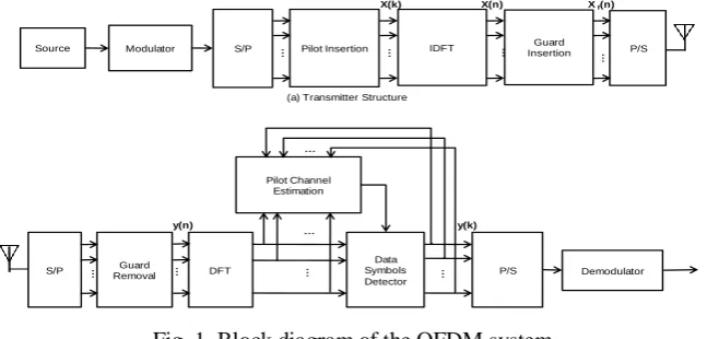
The OFDM baseband system based on iterative channel estimation is shown in the Fig.1. Unlike traditional OFDM baseband system, the detected symbols are feed back as additional pilot to improve the channel estimation. Assume that there are N sub-carriers in one OFDM symbol.

Source Modulator S/P Pilot Insertion IDFT _InsertionGuard P/S

(a) Transmitter Structure

… … … _…

S/P _RemovalGuard DFT P/S Demodulator

Data Symbols Detector

… … … …

Pilot Channel Estimation

…

…

X(n)

X(k) X f(n)

y(n) y(k)

Fig. 1. Block diagram of the OFDM system

As can be shown in Fig.1, the modulated signal {X k( )}is transformed into time domain signal

{

x( )

n

} with the following equation:

1

0

x ( )

{

( ) } n = 0 , 1 , 2 , . . . , N - 1

1

2

( ) exp( (

)

)

N

K

n

IDFT X k

X k

j

nk

N

N















(1)

N is the DFT length.

(

) , n = - N , - N

1 , . . . , 1

( )

( ), n = 0,1,...,N-1

g g

f

x N

n

x n

x n









 



₍₂₎

Where Ng is the length of CP.

After removing the CP, the sampled received signal can be characterized in the following equation [12]:

1 0

( )

( , )

(

)

( )

L f l

y n

h n l x n l

w n









 

(3)

Where w(n) is the additive white Gaussian noise (AWGN) with zero mean and

variance



2_w.h n l( , ) is the fading coefficient of the

l

th path at time n. The wireless channel coefficients matrix H can be denoted as follow:

H

























0,0 0,L-1 0,L-2 0,1

1,1 1,0 1,L-1 1,2

N-1,L-1 N-1,L-2 N-1,0

h

0

0

...

h

h

...

h

h

h

0

...

0

h

...

h

=

...

...

...

...

...

...

...

...

0

0

0

... h

h

... h

(4) Assume that the wireless channel follow the Jakes Model, then h n l( , )and h m l( , )are

correlative [15], the correlation isE h n l h m l{ ( , ) ( , )*}a J_l. (2 ( - )₀ p n m f T_{m s}).Where J₀

(.)

is the first

class of Bessel function, Ts is the sample time,

f

_mis the maximum Doppler spread,



_l is the

mean power of the

l

th _path.

The demodulated signal in frequency domain is obtained by taking N-point DFT of y (n) as [12]:

1 1

(2 / )

, ,

0 , 0

Component

1

( )

( )

( )

( )

( )

N N

j N kn

k k m k

n m k m

ICI

Y k

y n e

H

X k

H

m

W k

N

      













(5) where

1 1 1

2 /

,

0 0 0

1

1

( , )

( )

N L N

j lm N

k k k

n l n

H

h n l e

h n

N

N

       









(6)

1 1 1

2 / 2 ( ) / 2 ( ) /

,

n 0 0 n 0

1

1

( , )

( )

N L N

j lk N j k m n N j k m n N

m k k

l

H

h n l e

e

h n e

N

N

             







_

_







 



(7) 1

( 2 / )

0

1

( )

( )

N

j N n k

n

W k

w n e

N

   





(8)

Note that if the channel is time-invariant during one OFDM symbol period, the value of (7) is

zero (

2 1

0

0,

1,...,

1

j nk N

N

n

e

k

N



 









disappears. However, in the high mobility OFDM systems, the Doppler spread makes it no long true.

As the channel matrix H can be expressed as H=FHhF, the receiver signal after DFT is represented as [12]

Y



HX



W

(9)

Where F is the NN discrete Fourier transform (DFT) matrix whose entry at row n and

column k is denoted as

2 ,

j nk N n k

w e

 

 .In the wireless channel matrix H, the entry at row n and

column m



_n,mis denoted as

1

,m , ,

0

, 0

L

n n m l m l

H w











（n, m）N- 1 .For a time-invariant channel,

channel estimation only need to estimate the diagram entry as the non-diagram entry of the H matrix is zero. However, for a time-variant fading channel, the value of (7) is not zero, ICI makes the channel estimation inaccurate. So in high mobility scenarios, incorporate the Doppler spread makes the results of channel estimation more accurate.

3 Iterative Doppler-assisted channel estimation

As proved in [11], using the Doppler spread in the receiver mitigated the ICI and made the channel estimation accurate. The algorithm in [14] is optimized by proposing an improved iterative channel estimation algorithm combined with the Doppler information of the receiver.

To estimate the wireless channel, comp-type pilots are inserted into every OFDM symbol in the transmitter. First, the pilot channel coefficients are iteratively estimated by using pilot tones. A time-domain interpolation and LS method are employed to obtain channel estimates from the pilot tones. During the iteration process, the detected data symbols at the receiver are fed back to the channel estimator as additional pilot tones. These symbols, together with the pilot symbols are used to estimate the pilot channel coefficients. Thus the pilot channel coefficients are refined iteratively by using both the pilot and data symbols. The estimate of each data channel coefficient is obtained by a weighted time-domain interpolation of the selected pilot channel coefficients. The interpolation weights are designed based on the Doppler spread information of the receiver. The Doppler spread can be calculated by the velocity of the receiver.

3.1 Estimation of the data channel coefficients

To estimate the data channel coefficients, the pilot channel coefficients which have the maximum correlation with the specific data channel coefficients are selected. Then each of the selected pilot channel coefficients is weighted. The weight of each pilot channel coefficient is

designed based on the Doppler information of the receiver. Assume M_n{m_n,1,...,m_{n M,} }

denotes the set of the pilot sub-carriers used to express

~

h(l,n)

in the interpolation process, where

,

h( ,l mn k)is the channel impulse response of th

l

_{tap in sub-carrier}

,

n k

m

.

a

Tn denotes the

( , )

a [ ( ,

,1

),..., ( ,

,

)]

T T

n n n M

h l n



h l m

h l m

(10)

3.2 Calculation of the interpolation weights

As discussed in the section 2, the wireless channel coefficients follow the Jake’s model. The

correlation between h n l( , )and h m l( , )isE h n l h m l{ ( , ) ( , )*}a J_l. (2 ( - )₀ p n m f T_{m s}). To minimize

the channel estimation error

~ 2

[| ( , )

_nH

( ) | ]

E h l n



a h l

,

a

_nHis obtained by using the orthogonality principle as

1

, ,

a

n

H

n

R

n h h

R

n h h 



(11)

Where

n 0 n,1 0 n,M

n,h h

R

= [J [m

- n], ..., J [m

- n]]

(12)

























0 n,1 n,1 0 n,1 n,M

0 n,2 n,1 0 n,2 n,M

n,hh

0 n,M n,1 0 n,M n,M

J [m

- m ]

...

J [m

- m

]

J [m

- m ]

...

J [m

- m

]

R

=

...

...

...

J [m

- m ] ...

J [m

- m

]

(13)

3.3 Pilot iterative channel estimation

Assume in the tth iteration, the detected data symbol Xt-1 is known at the receiver. Substituting

,

k k

H

and

H

_{m k,} in (5) with (6) and (7), (5) can be expressed as

1

, ( 1 )

1 0 0

( ) ( ,

)

( )

(

)

p i l o t p i

N

N L

p s t

p p i p

s l i

b

l h l p X

s

e p





  



 

Y( p ) =

(14)

Where

e p

(

_p

)

denotes the estimation error at pilot sub-carrier

p

_p and AWGN noise. p,

i

p s p

b

is

the multiplex index. Note that in (10)

h l n

( , )

is expressed as weighted interpolation of

,1 ,

( ,

n

),..., ( ,

n M

)

h l m

h l m

, thus we can define a 1*L vector:

i i i

m,s m,s m,s

p p p

b

= [b

(0),...,b

(L -1)]

(15)

Substituting (14) with (15), (14) can be written as

1

1 ,

0 1

(

)

( )

b

(

)

pilot

i

N N

t m s

p p pi p

s i

Y P

X

s

h

e p

 

 









(16)

By extending the definition of (14) into a 1*LN pilot vector ,

[b

,

,..., b

,

]

pilot

m s m s m s

pN

b



, (16) can be

1

1

, 1

1

(

)

( )

p

(

)

t pp

N

p s t

p

p p

s

g

Y P

X

s b

h

e p



 









(17)

Where

pilot

T T T

p _{1 N}

h = [h , ..., h

]

.

(17) can be written as a linear equation

1

( ) )

( )

t_p p

(

Y p



G h





e p

(18)

Where ( ) [ ( ₁),..., ( )]

pilot

T N

Y p  Y p Y p

1

1 1 1

( )

[

,...,

]

N pilot

t t t T

p p p

G





g



g



( )

[ (

1

),..., (

_pilot

)]

T N

e p



e p

e p

.

Therefore,

~t

p

h

can be estimated by LS method:

1 1

( )

(

)

( )

t _t

p _p

h



G

 

Y p

(19) Once the pilot channel coefficients are estimated in the tth iteration by using (19), all the entries of the tth estimate of H in (4), can be calculated by using (10),(6),(7). The signal detection is

finished by performing zero-forcing as

t

t -1

X =(H ) Y

.The process will run continuously until the

end of the iteration.

4 Simulation Results

Simulations were carried out to verify the performance of the proposed iterative channel estimation method, and compared with the scheme in [11]. For comparing the performance of the proposed algorithm with perfect channel estimation, the system is simulated in which receivers are static and full channel state information is available in the receivers. The system parameters of the simulation are given in table 1 and table 2.

Table 1 Parameters of system simulation

Parameter s

Modulatio n

Carrier

frequency FFT Size

Data sub-carrier

Pilot

sub-carrier Sample Time

Value QPSK 5GHz 512 240 48 0.16us

Table 2 Max Doppler spread shift of simulation

The BER performances of the proposed iterative technique for variable numbers of iterations are given in Fig.2. It can be seen that the scheme converges after 5 iterations.

Velocity of the receiver Maximum Doppler spread(normalized) 80Km/h

300Km/h

1 2 3 4 5 6 7 0.005

0.01 0.015 0.02 0.025 0.03 0.035 0.04 0.045 0.05

Iteration Number

BER

SNR = 15 SNR = 20

Fig. 2. Convergence characteristic of the proposed iterative scheme

Fig.3 compares the BER performance of the proposed algorithm with the scheme in [11] for the normalized Doppler spread of 0.025. Note that the BER performance is similar. That is because when the Doppler is small, the channel is time-invariant. So the proposed algorithm has a comparative performance with other schemes.

0 5 10 15 20 25 30 10-4

10-3 10-2 10-1 100

SNR(dB)

BER

perfect channel estimation Proposed algorithm,Doppler spread 0.025 Traditional scheme, Doppler spread 0.025

Fig.3. The BER performance for the normalized Doppler spread of 0.025

Fig.4 compares the BER performance of the proposed algorithm with the scheme in [11] for the normalized Doppler spread of 0.1. As table 2 shows, the receiver moves at a speed higher than 300km/h. As shown in Fig.4, when the Doppler spread is 0.1, the BER performance of the proposed algorithm has been proved more than 2dB gain compared with the scheme in [11] .We can also note that the proposed algorithm is stable, for the BER performance for Doppler spread of 0.1 is similar with Doppler spread of 0.025, nearly achieves the performance as good as the perfect channel estimation.

0 5 10 15 20 25 30 10-4

10-3 10-2 10-1 100

SNR(dB)

BER

Perfect Channel estimation Proposed algorithm, Doppler spread 0 Proposed algorithm,Doppler spread 0.1 Conventional scheme,Doppler spread 0.1

5 Conclusions

In this paper, the ICI in the high mobility OFDM systems are analyzed. An improved iterative channel estimation algorithm is proposed for the systems. The proposed method have taken account of the time-variation in the channel estimation process, and the detected symbols are fed back as additional pilot tones to refine the channel estimation results.

The simulation performances show that the proposed algorithm performs better than conventional schemes. In the time-invariant scenario, the proposed scheme can nearly achieve the performance as good as perfect channel estimation. Especially in high mobility OFDM systems, that the Doppler spread normalized factor is 0.1, the BER performance is only 2dB weaker than the Doppler spread of 0. It is also only 3dB weaker than the perfect channel estimation. In conclusion, the performance of the proposed channel estimation algorithm is prior to that of the existing schemes.

Reference

[1] Leonard J.Cimini, Jr. Analysis and simulation of a digital mobile channel using orthogonal frequency-division multiplexing[J].

IEEE Trans Communication, 1985, 33(7): 665-675.

[2] Std.TR 25.814, Rev.7.1.0, Sep.2006.3GPP, Physical layer aspects for evolved UTRA[S].

[3] Std., Rev.2, 2006.IEEE, IEEE STD 802.16e-2005[S].

[4] Y.Li,J.H.Winters, N.R.Sollenberger. MIMO-OFDM for wireless communications, signal detection with enhanced channel

estimation[J]. IEEE Trans Communication, 2002, 50(7):1471-77.

[5] Zhang Ji-Dong , Zhen Bao-Yu. Channel estimation for OFDM systems based on pilot arrangement[J]. Transactions on Communication, 2003, 24(11):116-124.

[6] H. Meng-Han, W. Che-Ho. Channel estimation for OFDM systems based on comb-type pilot arrangment in frequency selective fading channels[J]. IEEE Transactions on Consumers Electronics, 1998, 44(5):217–225.

[7] S. Coleri, M. Ergen, A. Puri, A. Bahai. Channel estimation techniques based on pilot arrangement in OFDM systems[J]. IEEE Transactions on broadcasting, 2002, 48(3):223–229.

[8] O.Edfors, M.Sandell, J.J.Van dee Beek. OFDM channel estimation by singular value decomposition[J]. IEEE Trans on

Communication, 1998, 46(5):931-939.

[9] L.ye, N.Sehadri, N.R.Sollenberger. Robust channel estimation for OFDM systems with transmitter diversity in mobility wire less

channels[J]. IEEE Trans on Communication, 1998, 46(7):902-915.

[10] Y. Mostofi ,D. Cox. ICI mitigation for pilot-aided OFDM mobile systems[J]. IEEE Transactions on Wireless Communications, 2005, 4(8): 765–774.

[11] A.Stamoulis, S.Diggavi, N.Al-dhahir. Inter-carrier interference in MIMO-OFDM[J]. IEEE Transactions on signal processing, 2002, 50(10):2451-2464.

[12] M.Zhao, Z.Shi, M.Reed. Iterative turbo channel estimation for ofdm system over rapid dispersive fading channel[J]. IEEE Trans on Wireless Communication, 2007, 7(8):2226-2238.

[13] S.Marinkovic, B.Vucetic, A.Ushirokawa. Spacetime iterative and multistage receiver structures for cdma mobile communication

systems[j]. IEEE J.Sel. Areas Communication,2001,19(8):1594-1604.

[14] W.Hardjawana, R.Li, B.Vucetic. A new iterative channel estimation for high mobility MIMO-OFDM systems[C]. VTC, May

2010.