Support Vector Machinery for Infinite Ensemble Learning

Support Vector Machinery for Infinite Ensemble Learning

Hsuan-Tien Lin [email protected]

Ling Li [email protected]

Department of Computer Science California Institute of Technology Pasadena, CA 91125, USA

Editor: Peter L. Bartlett

Abstract

Ensemble learning algorithms such as boosting can achieve better performance by averaging over the predictions of some base hypotheses. Nevertheless, most existing algorithms are limited to combining only a finite number of hypotheses, and the generated ensemble is usually sparse. Thus, it is not clear whether we should construct an ensemble classifier with a larger or even an infinite number of hypotheses. In addition, constructing an infinite ensemble itself is a challenging task. In this paper, we formulate an infinite ensemble learning framework based on the support vector machine (SVM). The framework can output an infinite and nonsparse ensemble through embed-ding infinitely many hypotheses into an SVM kernel. We use the framework to derive two novel kernels, the stump kernel and the perceptron kernel. The stump kernel embodies infinitely many decision stumps, and the perceptron kernel embodies infinitely many perceptrons. We also show that the Laplacian radial basis function kernel embodies infinitely many decision trees, and can thus be explained through infinite ensemble learning. Experimental results show that SVM with these kernels is superior to boosting with the same base hypothesis set. In addition, SVM with the stump kernel or the perceptron kernel performs similarly to SVM with the Gaussian radial basis function kernel, but enjoys the benefit of faster parameter selection. These properties make the novel kernels favorable choices in practice.

Keywords: ensemble learning, boosting, support vector machine, kernel

1. Introduction

Ensemble learning algorithms, such as boosting (Freund and Schapire, 1996), are successful in prac-tice (Meir and R¨atsch, 2003). They construct a classifier that averages over some base hypotheses in a set

H

. While the size of

H

can be infinite, most existing algorithms use only a finite subset of

H

, and the classifier is effectively a finite ensemble of hypotheses. Some theories show that the finite-ness places a restriction on the capacity of the ensemble (Freund and Schapire, 1997), and some theories suggest that the performance of boosting can be linked to its asymptotic behavior when the ensemble is allowed to be of an infinite size (R¨atsch et al., 2001). Thus, it is possible that an infinite ensemble is superior for learning. Nevertheless, the possibility has not been fully explored because constructing such an ensemble is a challenging task (Vapnik, 1998).

Such a framework can be applied both to construct new kernels for SVM, and to interpret some existing ones (Lin, 2005). Furthermore, the framework allows us to compare SVM and ensemble learning algorithms in a fair manner using the same base hypothesis set.

Based on the framework, we derive two novel SVM kernels, the stump kernel and the percep-tron kernel, from an ensemble learning perspective (Lin and Li, 2005a). The stump kernel embodies infinitely many decision stumps, and as a consequence measures the similarity between examples by the`1-norm distance. The perceptron kernel embodies infinitely many perceptrons, and works with the`2-norm distance. While there exist similar kernels in literature, our derivation from an ensemble learning perspective is nevertheless original. Our work not only provides a feature-space view of their theoretical properties, but also broadens their use in practice. Experimental results show that SVM with these kernels is superior to successful ensemble learning algorithms with the same base hypothesis set. These results reveal some weakness in traditional ensemble learn-ing algorithms, and help understand both SVM and ensemble learnlearn-ing better. In addition, SVM with these kernels shares similar performance to SVM with the popular Gaussian radial basis func-tion (Gaussian-RBF) kernel, but enjoys the benefit of faster parameter selecfunc-tion. These properties make the two kernels favorable choices in practice.

We also show that the Laplacian-RBF kernel embodies infinitely many decision trees, and hence can be viewed as an instance of the framework. Experimentally, SVM with the Laplacian-RBF ker-nel performs better than ensemble learning algorithms with decision trees. In addition, our deriva-tion from an ensemble learning perspective helps to explain the success of the kernel on some specific applications (Chapelle et al., 1999).

The paper is organized as follows. In Section 2, we review the connections between SVM and ensemble learning. Next in Section 3, we propose the framework for embedding an infinite number of hypotheses into a kernel. We then derive the stump kernel in Section 4, the perceptron kernel in Section 5, and the Laplacian-RBF kernel in Section 6. Finally, we show the experimental results in Section 7, and conclude in Section 8.

2. Support Vector Machine and Ensemble Learning

In this section, we first introduce the basics of SVM and ensemble learning. Then, we review some established connections between the two in literature.

2.1 Support Vector Machine

Given a training set_{(xi,yi)}_iN₌₁, which contains input vectors xi∈

X

⊆RDand their corresponding

labels yi∈ {−1,+1}, the soft-margin SVM (Vapnik, 1998) constructs a classifier

g(x) =sign _hw,φxi+b

from the optimal solution to the following problem:1 (P1) min

w_∈F,b_∈R,ξ_∈RN

1

2hw,wi+C

N

∑

i=1

ξi

s.t. yi hw,φxii+b

≥1₋ξi, for i=1,2, . . . ,N, ξi≥0, for i=1,2, . . . ,N.

Here C>0 is the regularization parameter, and φx =Φ(x) is obtained from the feature

map-pingΦ:

X

_→

F

. We assume the feature space

F

to be a Hilbert space equipped with the inner product _h·,_·i (Sch¨olkopf and Smola, 2002). Because

F

can be of an infinite number of dimen-sions, SVM solvers usually work on the dual problem:

(P2) min

λ∈RN

1 2

N

∑

i=1

N

∑

j=1

λiλjyiyj

K

(xi,xj)− N

∑

i=1

λi

s.t. 0_≤λi≤C, for i=1,2, . . . ,N, N

∑

i=1

yiλi=0.

Here

K

is the kernel function defined as

K

(x,x0) =_hφx,φx0i. Then, the optimal classifier becomes

g(x) =sign

N

∑

i=1

yiλiK(xi,x) +b !

, (1)

where b can be computed through the primal-dual relationship (Vapnik, 1998; Sch ¨olkopf and Smola, 2002).

The use of a kernel function

K

instead of computing the inner product directly in

F

is called the kernel trick, which works when

K

(_·,_·)can be computed efficiently (Sch ¨olkopf and Smola, 2002). Alternatively, we can begin with an arbitrary

K

, and check whether there exists a space-mapping pair(

F

,Φ)such that

K

(_·,_·)is a valid inner product in

F

. A key tool here is the Mercer’s condition, which states that a symmetric

K

(_·,_·) is a valid inner product if and only if its Gram matrix K, defined by Ki,j =

K

(xi,xj), is always positive semi-definite (PSD) (Vapnik, 1998; Sch ¨olkopf and

Smola, 2002).

The soft-margin SVM originates from the hard-margin SVM, which forces the margin viola-tionsξito be zero. When such a solution is feasible for(P1), the corresponding dual solution can be obtained by setting C to∞in(P2).

2.2 Adaptive Boosting and Linear Programming Boosting

The adaptive boosting (AdaBoost) algorithm (Freund and Schapire, 1996) is perhaps the most pop-ular and successful approach for ensemble learning. For a given integer T and a hypothesis set

H

, AdaBoost iteratively selects T hypotheses ht ∈

H

and weights wt ≥0 to construct an ensemble

classifier

gT(x) =sign T

∑

t=1 wtht(x)

!

.

The underlying algorithm for selecting ht ∈

H

is called a base learner. Under some

assump-tions (R¨atsch et al., 2001), it is shown that when T_→∞, AdaBoost asymptotically approximates an infinite ensemble classifier

g∞(x) =sign

∞

∑

t=1 wtht(x)

!

such that(w,h)is an optimal solution to

(P3) min

wt∈R,ht∈H

∞

∑

t=1 wt

s.t. yi

∞

∑

t=1

wtht(xi) !

≥1, for i=1,2, . . . ,N,

wt ≥0, for t=1,2, . . . ,∞.

Note that there are infinitely many variables in(P3). In order to approximate the optimal solution well with a fixed and finite T , AdaBoost resorts to two related properties of some of the optimal solutions for(P3): finiteness and sparsity.

• Finiteness: When two hypotheses have the same prediction patterns on the training input vectors, they can be used interchangeably during the training time, and are thus ambiguous. Since there are at most 2Nprediction patterns on N training input vectors, we can partition

H

into at most 2N groups, each of which contains mutually ambiguous hypotheses. Some opti-mal solutions of(P3)only assign one or a few nonzero weights within each group (Demiriz et al., 2002). Thus, it is possible to work on a finite data-dependent subset of

H

instead of

H

itself without losing optimality.

• Sparsity: Minimizing the `1-norm_kw_k1=∑∞_t=1|wt|often leads to sparse solutions (Meir

and R¨atsch, 2003; Rosset et al., 2007). That is, for hypotheses in the finite (but possibly still large) subset of

H

, only a small number of weights needs to be nonzero. AdaBoost can be viewed as a stepwise greedy search algorithm that approximates such a finite and sparse ensemble (Rosset et al., 2004).

Another boosting approach, called the linear programming boosting (LPBoost), can solve(P3) exactly. We will introduce the soft-margin LPBoost, which constructs an ensemble classifier like (2) with the optimal solution to

(P4) min

wt∈R,ht∈H

∞

∑

t=1 wt+C

N

∑

i=1

ξi

s.t. yi

∞

∑

t=1

wtht(xi) !

≥1₋ξi, for i=1,2, . . . ,N,

ξi≥0, for i=1,2, . . . ,N,

wt ≥0, for t=1,2, . . . ,∞.

Demiriz et al. (2002) proposed to solve(P4)with the column generating technique.2 The algorithm works by adding one unambiguous ht to the ensemble in each iteration. Because of the finiteness

property, the algorithm is guaranteed to terminate within T _≤2N iterations. The sparsity property can sometimes help speed up the convergence of the algorithm.

R¨atsch et al. (2002) worked on a variant of(P4)for regression problems, and discussed optimal-ity conditions when

H

is of infinite size. Their results can be applied to(P4)as well. In particular,

they showed that even without the finiteness property (e.g., when ht outputs real values rather than

binary values), (P4) can still be solved using a finite subset of

H

that is associated with nonzero weights. The results justify the use of the column generating technique above, as well as a barrier, AdaBoost-like, approach that they proposed.

Recently, Rosset et al. (2007) studied the existence of a sparse solution when solving a gen-eralized form of (P4) with some

H

of infinite and possibly uncountable size. They showed that under some assumptions, there exists an optimal solution of(P4)such that at most N+1 weights are nonzero. Thus, iterative algorithms that keep adding necessary hypotheses ht to the

ensem-ble, such as the proposed path-following approach (Rosset et al., 2007) or the column generating technique (Demiriz et al., 2002; R¨atsch et al., 2002), could work by aiming towards such a sparse solution.

Note that even though the findings above indicate that it is possible to design good algorithms to return an optimal solution when

H

is infinitely large, the resulting ensemble relies on the sparsity property, and is effectively of only finite size. Nevertheless, it is not clear whether the performance could be improved if either or both the finiteness and the sparsity restrictions are removed.

2.3 Connecting Support Vector Machine to Ensemble Learning

The connection between AdaBoost, LPBoost, and SVM is well-known in literature (Freund and Schapire, 1999; R¨atsch et al., 2001; R¨atsch et al., 2002; Demiriz et al., 2002). Consider the feature transform

Φ(x) = h1(x),h2(x), . . .

. (3)

We can see that the problem (P1) with this feature transform is similar to (P4). The elements of φx in SVM are similar to the hypotheses ht(x) in AdaBoost and LPBoost. They all work on

linear combinations of these elements, though SVM deals with an additional intercept term b. SVM minimizes the`2-norm of the weights while AdaBoost and LPBoost work on the`1-norm. SVM and LPBoost introduce slack variablesξi and use the parameter C for regularization, while AdaBoost

relies on the choice of the parameter T (Rosset et al., 2004). Note that AdaBoost and LPBoost require wt ≥0 for ensemble learning.

Several researchers developed interesting results based on the connection. For example, R ¨atsch et al. (2001) proposed to select the hypotheses ht by AdaBoost and to obtain the weights wt by

solving an optimization problem similar to(P1)in order to improve the robustness of AdaBoost. Another work by R¨atsch et al. (2002) introduced a new density estimation algorithm based on the connection. Rosset et al. (2004) applied the similarity to compare SVM with boosting algorithms. Nevertheless, as limited as AdaBoost and LPBoost, their results could use only a finite subset of

H

when constructing the feature mapping (3). One reason is that the infinite number of variables wt

and constraints wt≥0 are difficult to handle. We will show the remedies for these difficulties in the

next section.

3. SVM-Based Framework for Infinite Ensemble Learning

Vapnik (1998) proposed a challenging task of designing an algorithm that actually generates an infi-nite ensemble classifier, that is, an ensemble classifier with infiinfi-nitely many nonzero wt. Traditional

We solved the challenge via another route: the connection between SVM and ensemble learning. The connection allows us to formulate a kernel that embodies all the hypotheses in

H

. Then, the classifier (1) obtained from SVM with the kernel is a linear combination over

H

(with an intercept term). Nevertheless, there are still two main obstacles. One is to actually derive the kernel, and the other is to handle the constraints wt ≥0 to make (1) an ensemble classifier. In this section, we

combine several ideas to deal with these obstacles, and conquer Vapnik’s task with a novel SVM-based framework for infinite ensemble learning.

3.1 Embedding Hypotheses into the Kernel

We start by embedding the infinite number of hypotheses in

H

into an SVM kernel. We have shown in (3) that we could construct a feature mapping from

H

. The idea is extended to a more general form for deriving a kernel in Definition 1.

Definition 1 Assume that

H

=_{hα:α_∈

C

_}, where

C

is a measure space. The kernel that embod-ies

H

is defined as

K

H,r(x,x0) =

Z

Cφx(α)φx0(α)dα, (4)

whereφx(α) =r(α)hα(x), and r :

C

→R+is chosen such that the integral exists for all x,x0∈

X

.

Hereαis the parameter of the hypothesis h_α. Although two hypotheses with differentαvalues may have the same input-output relation, we would treat them as different objects in our framework. We shall denote

K

_H,r by

K

_H when r is clear from the context. The validity of the definition is formalized in the following theorem.

Theorem 2 Consider the kernel

K

_H in Definition 1.

1. The kernel is an inner product forφxandφx0 in the Hilbert space

F

=

L

₂(

C

), which contains

functionsϕ(_·):

C

_→R_{that are square integrable.}

2. For a set of input vectors_{xi}Ni=1∈

X

N, the Gram matrix of

K

H is PSD.

Proof The first part is known in mathematical analysis (Reed and Simon, 1980), and the second part follows Mercer’s condition.

3.2 Negation Completeness and Constant Hypotheses

When we use

K

_H in(P2), the primal problem(P1)becomes (P5) min

w∈L2(C),b∈R,ξ∈RN 1 2

Z

Cw

2_(α)dα+C

∑

N

i=1

ξi

s.t. yi

Z

Cw(α)r(α)hα(xi)dα+b

≥1₋ξi, for i=1,2, . . . ,N,

ξi≥0, for i=1,2, . . . ,N.

In particular, the classifier obtained after solving(P2)with

K

_H is the same as the classifier obtained after solving(P5):

g(x) =sign

Z

Cw(α)r(α)hα(x)dα+b

. (5)

When

C

is uncountable, it is possible that each hypothesis hαonly takes an infinitesimal weight w(α)r(α)dα

in the ensemble. Thus, the classifier (5) is very different from those obtained with traditional ensemble learning, and will be discussed further in Subsection 4.2.

Note that the classifier (5) is not an ensemble classifier yet, because we do not have the con-straints w(α)_≥0, and we have an additional term b. Next, we would explain that such a classifier is equivalent to an ensemble classifier under some reasonable assumptions.

We start from the constraints w(α)_≥0, which cannot be directly considered in (P1). Vapnik (1998) showed that even if we add a countably infinite number of constraints to (P1), infinitely many variables and constraints would be introduced to(P2). Then, the latter problem would still be difficult to solve.

One remedy is to assume that

H

is negation complete, that is,3 h_∈

H

_⇔(₋h)_∈

H

.

Then, every linear combination over

H

has an equivalent linear combination with only nonnegative weights. Negation completeness is usually a mild assumption for a reasonable

H

(R ¨atsch et al., 2002). Following this assumption, the classifier (5) can be interpreted as an ensemble classifier over

H

with an intercept term b. Somehow b can be viewed as the weight on a constant hypothesis c, which always predicts c(x) =1 for all x_∈

X

. We shall further add a mild assumption that

H

contains both c and(₋c). Then, the classifier (5) or (1) is indeed equivalent to an ensemble classifier.

We summarize our framework in Algorithm 1. The framework shall generally inherit the pro-found performance of SVM. Most of the steps in the framework can be done by existing SVM implementations, and the hard part is mostly in obtaining the kernel

K

_H. In the next sections, we derive some concrete instances using different base hypothesis sets.

4. Stump Kernel

In this section, we present the stump kernel, which embodies infinitely many decision stumps. The decision stump sq,d,α(x) =q·sign (x)d−α

works on the d-th element of x, and classifies x according to q_{∈ {−}1,+1_}and the thresholdα(Holte, 1993). It is widely used for ensemble learning because of its simplicity (Freund and Schapire, 1996).

1. Consider a training set_{(xi,yi)}Ni=1and the hypothesis set

H

, which is assumed to be negation complete and to contain a constant hypothesis.

2. Construct a kernel

K

_H according to Definition 1 with a proper embedding function r. 3. Choose proper parameters, such as the soft-margin parameter C.

4. Solve(P2)with

K

H and obtain Lagrange multipliersλi and the intercept term b.

5. Output the classifier

g(x) =sign

N

∑

i=1

yiλi

K

H(xi,x) +b !

,

which is equivalent to some ensemble classifier over

H

.

Algorithm 1: SVM-based framework for infinite ensemble learning

4.1 Formulation and Properties

To construct the stump kernel, we consider the following set of decision stumps

S

=

sq,d,αd: q∈ {−1,+1},d∈ {1, . . . ,D},αd∈[Ld,Rd] .

We also assume

X

_⊆(L1,R1)×(L2,R2)× ··· ×(LD,RD). Thus, the set

S

is negation complete and

contains s+1,1,L1 as a constant hypothesis. The stump kernel

K

S defined below can then be used in Algorithm 1 to obtain an infinite ensemble of decision stumps.

Definition 3 The stump kernel is

K

S with r(q,d,αd) =rS =1₂,

K

S(x,x0) =∆S−

D

∑

d=1

(x)_d−(x0)_d

=∆S−

x−x0

1, where∆S= 1₂∑D_d=1(Rd−Ld)is a constant.

Definition 3 is a concrete instance that follows Definition 1. The details of the derivation are shown in Appendix A. As we shall see further in Section 5, scaling r_S is equivalent to scaling the param-eter C in SVM. Thus, without loss of generality, we use r_S = 1

2 to obtain a cosmetically cleaner kernel function.

The validity of the stump kernel follows directly from Theorem 2 of the general framework. That is, the stump kernel is an inner product in a Hilbert space of some square integrable func-tionsϕ(q,d,αd), and it produces a PSD Gram matrix for any set of input vectors {xi}Ni=1∈

X

N. Given the ranges (Ld,Rd), the stump kernel is very simple to compute. Furthermore, the ranges

are not even necessary in general, because dropping the constant∆_S does not affect the classifier obtained from SVM.

Proof We extend from the results of Berg et al. (1984) to show that ˜

K

S(x,x0)is conditionally PSD (CPSD). In addition, because of the constraint∑N_i=1yiλi=0, a CPSD kernel ˜

K

(x,x0)works exactly

the same for(P2)as any PSD kernel of the form ˜

K

(x,x0) +∆, where∆is a constant (Sch ¨olkopf and Smola, 2002). The proof follows with∆=∆_S.

In fact, a kernel ˆ

K

(x,x0) =

K

˜(x,x0) +f(x) +f(x0)with any mapping f is equivalent to ˜

K

(x,x0) for(P2)because of the constraint∑iN=1yiλi=0. Now consider another kernel

ˆ

K

S(x,x0) =

_K

˜_S(x,x0_{) +}

∑

D

d=1 (x)d+

D

∑

d=1

(x0)d=2 D

∑

d=1

min((x)d,(x0)d).

We see that ˆ

K

_S, ˜

K

_S, and

K

_S are equivalent for(P2). The former is called the histogram intersection kernel (up to a scale of 2) when the elements(x)d represent generalized histogram counts, and has

been successfully used in image recognition applications (Barla et al., 2003; Boughorbel et al., 2005; Grauman and Darrell, 2005). The equivalence demonstrates the usefulness of the stump kernel on histogram-based features, which would be further discussed in Subsection 6.4. A remark here is that our proof for the PSD-ness of

K

S comes directly from the framework, and hence is simpler and more straightforward than the proof of Boughorbel et al. (2005) for the PSD-ness of ˆ

K

_S.

The simplified stump kernel is simple to compute, yet useful in the sense of dichotomizing the training set, which comes from the following positive definite (PD) property.

Theorem 5 (Lin, 2005) Consider training input vectors{xi}Ni=1∈

X

N. If there exists a dimension d such that(xi)d6= (xj)dfor all i6= j, the Gram matrix of

K

S is PD.

The PD-ness of the Gram matrix is directly connected to the classification capacity of the SVM classifiers. Chang and Lin (2001b) showed that when the Gram matrix of the kernel is PD, a hard-margin SVM with such a kernel can always dichotomize the training set perfectly. Keerthi and Lin (2003) then applied the result to show that SVM with the popular Gaussian-RBF kernel

K

(x,x0) = exp

−γkx₋x0_k2₂

can always dichotomize the training set when C_→ ∞. We obtain a similar theorem for the stump kernel.

Theorem 6 Under the assumption of Theorem 5, there exists some C∗>0 such that for all C_≥C∗, SVM with

K

_S can always dichotomize the training set_{(xi,yi)}Ni=1.

We make two remarks here. First, although the assumption of Theorem 6 is mild in practice, there are still some data sets that do not have this property. An example is the famous XORdata set (Figure 1). We can see that every possible decision stump makes 50% of errors on the training input vectors. Thus, AdaBoost and LPBoost would terminate with one bad decision stump in the ensemble. Similarly, SVM with the stump kernel cannot dichotomize this training set perfectly, regardless of the choice of C. Such a problem is inherent in any ensemble model that combines decision stumps, because the model belongs to the family of generalized additive models (Hastie and Tibshirani, 1990; Hastie et al., 2001), and hence cannot approximate non-additive target functions well.

-6

d d t

t

Figure 1: TheXORdata set

the Gaussian-RBF kernel, it has been known that SVM with reasonable parameter selection pro-vides suitable regularization and achieves good generalization performance even in the presence of noise (Keerthi and Lin, 2003; Hsu et al., 2003). We observe similar experimental results for the stump kernel (see Section 7).

4.2 Averaging Ambiguous Stumps

We have discussed in Subsection 2.2 that the set of hypotheses can be partitioned into groups and traditional ensemble learning algorithms can only pick a few representatives within each group. Our framework acts in a different way: the`2-norm objective function of SVM leads to an optimal solution that combines all the predictions within each group. This property is formalized in the following theorem.

Theorem 7 Consider two ambiguous h_α,h_β∈

H

. If the kernel

K

_H is used in Algorithm 1, the optimal w of(P5)satisfies w_r((_αα₎)=w_r((_ββ₎).

Proof The optimality condition between(P1)and(P2)leads to w(α)

r(α) =

N

∑

i=1

λihα(xi) = N

∑

i=1

λihβ(xi) =

w(β) r(β).

If w(α) is nonzero, w(β)would also be nonzero, which means both h_αand h_βare included in the ensemble. As a consequence, for each group of mutually ambiguous hypotheses, our framework considers the average prediction of all hypotheses as the consensus output.

The averaging process constructs a smooth representative for each group. In the following theorem, we demonstrate this behavior with the stump kernel, and show how the decision stumps group together in the final ensemble classifier.

Theorem 8 Define(x˜)d,a as the a-th smallest value in{(xi)d}N_i=1, and Ad as the number of

differ-ent(x˜)d,a. Let(x˜)d,0=Ld,(x˜)d,(Ad+1)=Rd, and

ˆ

sq,d,a(x) =q· 

 

 

+1, when(x)d≥(x˜)d,a+1; −1, when(x)d≤(x˜)d,a;

2(x)d−(x˜)d,a−(x˜)d,a+1

(x˜)d,a+1−(x˜)d,a , otherwise.

Then, for ˆr(q,d,a) =1 2

p

(x˜)d,a+1−(x˜)d,a,

K

S(xi,x) =

∑

q∈{−1,+1}

D

∑

d=1

Ad

∑

a=0

Proof First, for any fixed q and d, a simple integration shows that

Z (x˜)_d,a+1

(x˜)d,a

sq,d,α(x)dα =

(x˜)d,a+1−(x˜)d,a

ˆ

sq,d,a(x).

In addition, note that for allα_∈

(x˜)d,a,(x˜)d,a+1

, ˆsq,d,a(xi) =sq,d,α(xi). Thus,

Z R_d

Ld

r(q,d,α)sq,d,α(xi)

r(q,d,α)sq,d,α(x)

dα

=

Ad

∑

a=0

Z (x˜)d,a+1

(x˜)d,a

1

2sq,d,α(xi) 1

2sq,d,α(x)

dα

=

Ad

∑

a=0 1

4sˆq,d,a(xi)

Z (x˜)_d,a+1

(x˜)d,a

sq,d,α(x)dα

=

Ad

∑

a=0 1 4

(x˜)d,a+1−(x˜)d,a

ˆ

sq,d,a(xi)sˆq,d,a(x).

The theorem can be proved by summing over all q and d.

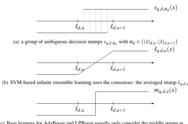
As shown in Figure 2, the function ˆsq,d,ais a smoother variant of the decision stump. Theorem 8

indicates that the infinite ensemble of decision stumps produced by our framework is equivalent to a finite ensemble of data-dependent and smoother variants. Another view of ˆsq,d,a is that they

are continuous piecewise linear functions (order-2 splines) with knots defined on the training fea-tures (Hastie et al., 2001). Then, Theorem 8 indicates that an infinite ensemble of decision stumps can be obtained by fitting an additive model of finite size using these special splines as the bases. Note that although the fitting problem is of finite size, the number of possible splines can grow as large as O(ND), which can sometimes be too large for iterative algorithms such as backfit-ting (Hastie et al., 2001). On the other hand, our SVM-based framework with the stump kernel can be thought as a route to solve this special spline fitting problem efficiently via the kernel trick.

As shown in the proof of Theorem 8, the averaged stump ˆsq,d,arepresents the group of

ambigu-ous decision stumps withαd∈

(x˜)d,a,(x˜)d,a+1

. When the group is larger, ˆsq,d,abecomes smoother.

Traditional ensemble learning algorithms like AdaBoost or LPBoost rely on a base learner to choose one decision stump as the only representative within each group, and the base learner usually returns the middle stump mq,d,a. As shown in Figure 2, the threshold of the middle stump is at the mean

of(x˜)d,aand(x˜)d,a+1. Our framework, on the other hand, enjoys a smoother decision by averaging

over more decision stumps. Even though each decision stump only has an infinitesimal hypothesis weight, the averaged stump ˆsq,d,ahas a concrete weight in the ensemble.

5. Perceptron Kernel

In this section, we extend the stump kernel to the perceptron kernel, which embodies infinitely many perceptrons. A perceptron is a linear threshold classifier of the form

p_θ,α(x) =sign θTx−α

-˜

xd,a x˜d,a+1

sq,d,αd(x)

(a) a group of ambiguous decision stumps sq,d,αdwithαd∈ (x˜)d,a,(x˜)d,a+1

-˜

xd,a x˜d,a+1

ˆ sq,d,a(x)

(b) SVM-based infinite ensemble learning uses the consensus: the averaged stump ˆsq,d,a

-˜

xd,a x˜d,a+1

mq,d,a(x)

(c) Base learners for AdaBoost and LPBoost usually only consider the middle stump mq,d,a

Figure 2: The averaged stump and the middle stump

It is a basic theoretical model for a neuron, and is very important for building neural networks (Haykin, 1999).

To construct the perceptron kernel, we consider the following set of perceptrons

P

=

pθ,α:θ∈RD,kθk2=1,α∈[−R,R] .

We assume that

X

is within the interior of

B

(R), where

B

(R) is a ball of radius R centered at the origin inRD_{. Then, the set}

P

_{is negation complete, and contains a constant hypothesis pe1,−R}

where e1= (1,0, . . . ,0)T. Thus, the perceptron kernel

K

P defined below can be used in Algorithm 1 to obtain an infinite ensemble of perceptrons.

Definition 9 Let

ΘD=

Z

kθk2=1

dθ, ΞD=

Z

kθk2=1

cos(anglehθ,e₁i)

dθ,

where the operator angle_h·,_·iis the angle between two vectors, and the integrals are calculated with uniform measure on the surface_kθ_k2=1. The perceptron kernel is

K

_P with r(θ,α) = r_P,

K

P(x,x0) =∆_P−

x−x0

2, where the constants r_P = (2ΞD)−

1

2 _and∆_P =Θ

DΞ−D1R.

computing the perceptron kernel for SVM. Williams (1998) mentioned that “Paradoxically, it may be easier to carry out Bayesian prediction with infinite networks rather than finite ones.” Similar claims can be made with ensemble learning.

The perceptron kernel shares many similar properties to the stump kernel. First, the constant∆P can also be dropped, as formalized below.

Theorem 10 Solving(P2)with the simplified perceptron kernel ˜

K

P(x,x0) =−kx−x0k2is the same as solving(P2)with

K

P(x,x0).

Second, SVM with the perceptron kernel can also dichotomize the training set perfectly, which comes from the usefulness of the simplified perceptron kernel ˜

K

_P in interpolation.

Theorem 11 (Micchelli, 1986) Consider input vectors_{xi}Ni=1∈

X

N, and the perceptron kernel

K

P in Definition 9. If xi6=xj for all i6= j, then the Gram matrix of

K

P is PD.

Then, similar to Theorem 6, we get the following result.

Theorem 12 If xi6=xjfor all i6=j, there exists some C∗>0 such that for all C≥C∗, SVM with

K

P

can always dichotomize the training set_{(xi,yi)}Ni=1.

Another important property, called scale-invariance, accompanies the simplified perceptron ker-nel, which was also named the triangular kernel by Fleuret and Sahbi (2003). They proved that when the kernel is used in the hard-margin SVM, scaling all training input vectors xi by some

positiveγdoes not change the optimal solution.

In fact, in the soft-margin SVM, a well-known result is that scaling the Gram matrix K by some γ>0 is equivalent to scaling C by γin(P2). Because the simplified perceptron kernel ˜

K

P satisfiesγ

K

˜_P(x,x0) =

K

˜_P(γx,γx0), the effect of scaling training examples can be equivalently per-formed with the parameter selection step on C. That is, when C is selected reasonably, there is no need to explicitly have a scaling parameterγ.

Recall that we construct the perceptron kernel (and the stump kernel) with an embedding con-stant r_P (and r_S), and from Definition 1, multiplying the constant by√γ>0 is equivalent to scaling the Gram matrix K byγ. Thus, when C is selected reasonably, there is also no need to explicitly try different r_P or r_S for these two kernels. We will further discuss the benefits of this property in Subsection 6.4.

6. Laplacian-RBF Kernel

6.1 Summation: Embedding Multiple Sets of Hypotheses

Summation can be used to embed multiple sets of hypotheses altogether. For example, given ker-nels

K

_H1 and

K

_H2, their summation

K

(x,x0) =

K

_H1(x,x0) +

K

_H2(x,x0)

embodies both

H

1 and

H

2. In other words, if we use

K

(x,x0) in Algorithm 1, we could obtain an ensemble classifier over

H

1∪

H

2when the union is negation complete and contains a constant hypothesis.

In traditional ensemble learning, when multiple sets of hypotheses are considered altogether, it is usually necessary to call a base learner for each set. On the other hand, our framework only requires a simple summation on the kernel evaluations. In fact, as shown in the next theorem, our framework can be applied to work with any countable sets of hypotheses, which may not be an easy task for traditional ensemble learning algorithms.

Theorem 13 Assume that the kernels

K

_H1, . . . ,

K

_HJ are defined for some J∈NS

{∞}with sets of hypotheses

H

1, . . . ,

HJ

, respectively. Then, let

K

(x,x0) =

J

∑

j=1

K

_Hj(x,x0).

If

K

(x,x0)exists for all x,x0_∈

X

, and

H

=SJ

j=1

H

j is negation complete and contains a constant

hypothesis, Algorithm 1 using

K

(x,x0)outputs an ensemble classifier over

H

.

Proof The theorem comes from the following result in mathematical analysis: any countable direct sum over Hilbert spaces is a Hilbert space (Reed and Simon, 1980, Example 5). Lin (2005, Theo-rem 6) showed the details of the proof.

A remark on Theorem 13 is that we do not intend to define a kernel with

H

directly. Otherwise we need to choose suitable

C

and r first, which may not be an easy task for such a complex hy-pothesis set. Using the summation of the kernels, on the other hand, allow us to obtain an ensemble classifier over the full union with less efforts.

6.2 Multiplication: Performing Logical Combination of Hypotheses

It is known that we can combine two kernels by point-wise multiplication to form a new ker-nel (Sch¨olkopf and Smola, 2002). When the two kerker-nels are associated with base hypothesis sets, a natural question is: what hypothesis set is embedded in the new kernel?

Next, let output+1 represent logic TRUE and₋1 represent logic FALSE. We show that multi-plication can be used to perform common logical combinations on the hypotheses.

Theorem 14 For two sets of hypotheses

H

1={hα:α∈

C

1}and

H

2=

h_β:β_∈

C

2 , define

H

=

h_α,β: hα,β(x) =−hα(x)·hβ(x),α∈

C

1,β∈

C

2 . In addition, let r(α,β) =r1(α)r2(β). Then,

K

H,r(x,x0) =

K

H1,r1(x,x 0_)·

_K

H2,r2(x,x 0₎

The proof simply follows from Definition 1. Note that when representing logic, the combined hypothesis h_α,βis the XOR operation on hαand hβ. More complicated results about other operations can be introduced under a mild assumption called neutrality.

Definition 15 A set of hypothesis

H

=_{hα:α_∈

C

_}is neutral to

X

with a given r if and only if for all x_∈

X

,R

α∈Chα(x)r2(α)dα=0.

Note that for a negation complete set

H

, neutrality is usually a mild assumption (e.g., by assign-ing the same r for hαand₋hα). We can easily verify that the set of decision stumps in Definition 3 and the set of perceptrons in Definition 9 are both neutral.

Theorem 16 For two sets of hypotheses

H

1={hα:α∈

C

1}and

H

2=

h_β:β_∈

C

2 , define

H

=

hq,α,β: hq,α,β(x) =q·min hα(x),hβ(x)

,α

∈

C

1,β∈

C

2,q∈ {−1,+1} . Assume that

H

1and

H

2are neutral with r1and r2, respectively, and both integrals

∆1=

Z

α∈C1

r2₁(α)dα,∆2=

Z

β∈C2

r2₂(β)dβ are finite. In addition, let r(q,α,β) =√2r1(α)r2(β). Then,

K

_H,r(x,x0) =

K

H1,r1(x,x 0_{) +∆}

1

·

K

H2,r2(x,x 0_{) +∆}

2

for all x,x0_∈

X

. Furthermore,

H

is neutral to

X

with r.

Proof Because h_α(x),h_β(x)_{∈ {−}1,+1_},

h₊1,α,β(x) = 1

2 hα(x)hβ(x) +hα(x) +hβ(x)−1

.

Then,

K

_H,r(x,x0)

= 2

Z

h+1,α,β(x)h+1,α,β(x0)r2(α,β)dβdα = 1

2

Z

hα(x)h_β(x) +hα(x) +h_β(x)₋1 hα(x0)h_β(x0) +hα(x0) +h_β(x0)₋1r2(α,β)dβdα =

Z

hα(x)h_β(x)hα(x0)h_β(x0) +hα(x)hα(x0) +h_β(x)h_β(x0) +1r2₁(α)r2₂(β)dβdα (6) =

K

_H1,r1(x,x

0_{) +∆} 1

·

K

H2,r2(x,x 0_{) +∆}

2

.

Note that (6) comes from the neutrality assumption, which implies that during integration, the cross-terms like

Z

h_α(x)h_β(x0)r₁2(α)r2₂(β)dαdβ are all 0. Neutrality of

H

follows from the symmetry in q.

6.3 Stump Region Kernel, Decision Tree Kernel, and Laplacian-RBF Kernel

Next, we use the stump kernel to demonstrate the usefulness of summation and multiplication. When

H

1=

H

2=

S

, the resulting

K

_H from Theorem 16 embodies AND/OR combinations of two decision stumps in

S

. Extending this concept, we get the following new kernels.

Definition 17 The L-level stump region kernel

K

_TL is recursively defined by

K

T1(x,x

0_{) =}

_K

_S(x,x0_{) +∆S,∆}

1=2∆S,

K

TL+1(x,x0) =

K

TL(x,x0) +∆L

K

S(x,x0) +∆_S

,∆L+1=2∆L∆S for L∈N.

If we construct a kernel from _{c,₋c_} with r=q1

2∆S on each hypothesis, we can see that the constant∆S is also a neutral kernel. Since neutrality is preserved by summation, the kernel

K

_T1 is neutral as well. By repeatedly applying Theorem 16 and maintaining∆Las the constant associated

with

TL

, we see that

K

_TL embodies all possible AND/OR combinations of L decision stumps in

S

. We call these hypotheses the L-level stump regions.

Note that we can solve the recurrence and get

K

TL(x,x0) = 2L∆L_S

L

∑

`=1

K

S(x,x0) +∆S 2∆_S

`

, for L_∈N_.

Then, by applying Theorem 13, we obtain an ensemble classifier over stump regions of any level.

Theorem 18 For 0<γ< _∆1

S, the infinite stump region (decision tree) kernel

K

T(x,x0) = exp γ_·

K

S(x,x0) +∆S−1

can be applied to Algorithm 1 to obtain an ensemble classifier over

T

=S∞

L=1

TL

. Proof By Taylor’s series expansion of exp(ε)nearε=0, we get

K

T(x,x0) =

∞

∑

L=1

γL

L!

K

S(x,x

0_{) +∆S}L

= γ

K

_T1(x,x0) +

∞

∑

L=2

γL

L!

K

TL(x,x

0_)−2∆S

_K

TL−1(x,x 0₎

=

∞

∑

L=1

γL

L!

K

TL(x,x 0₎₋

∑

∞

L=1

γL+1

(L+1)!2∆S

K

TL(x,x 0₎

=

∞

∑

L=1

γL

L!−

γL+1_2∆ S (L+1)!

K

TL(x,x0).

Note thatτL=γ L L!−

γL+1_2∆

S

(L+1)! >0 for all L≥1 if and only if 0<γ< 1

∆S. The desired result simply

follows Theorem 13 by scaling the r functions of each

K

_TLby√τL.

that output{−1,+1_}, that is, a decision tree (Quinlan, 1986; Hastie et al., 2001). In addition, we can view the nodes of a decision tree as logic operations:

tree

= OR(AND(root node condition,left),AND(NOT(root node condition),right)).

By recursively replacing each root node condition with a decision stump, we see that every decision tree can be represented as a stump region hypothesis. Thus, the set

T

that contains stump regions of any level is the same as the set of all possible decision trees, which leads to the name decision tree kernel.4

Decision trees are popular for ensemble learning, but traditional algorithms can only deal with trees of finite levels (Breiman, 1999; Dietterich, 2000). On the other hand, when the decision tree kernel

K

_T is plugged into our framework, it allows us to actually build an infinite ensemble over decision trees of arbitrary levels.

Note that the decision tree kernel

K

_T(x,x0)is of the form

κ1exp −κ2

x−x0

1

+κ3

whereκ1,κ2,κ3 are constants andκ1,κ2 are positive. We mentioned in Section 4 that scaling the kernel withκ1is equivalent to scaling the soft-margin parameter C in SVM, and in Theorem 4 that droppingκ3does not affect the solution obtained from SVM. Then, the kernel

K

T(x,x0)is similar to the Laplacian-RBF kernel

K

_L(x,x0) =exp(₋γ_kx₋x0_k1). This result is a novel interpretation of the Laplacian-RBF kernel: under suitable parameters, SVM with the Laplacian-RBF kernel allows us to obtain an infinite ensemble classifier over decision trees of any level.5

Not surprisingly, when all training input vectors xiare distinct (Micchelli, 1986; Baxter, 1991),

the Gram matrix of

K

L (and hence

K

_T) is PD. Then, the Laplacian-RBF kernel and the decision tree kernel could be used to dichotomize the training set perfectly.

6.4 Discussion on Radial Basis Function Kernels

Note that the stump kernel, the perceptron kernel, the Laplacian-RBF kernel, and the Gaussian-RBF kernel are all radial basis functions. They can all be used to dichotomize the training set perfectly under mild conditions, while the first three connect to explanations from an ensemble perspective. Next, we compare two properties of these kernels, and discuss their use in SVM applications.

First, we can group these kernels by the distance metrics they use. The stump kernel and the Laplacian-RBF kernel deal with the`1-norm distance between input vectors, while the others work on the`2-norm distance. An interesting property of using the`2-norm distance is the invariance to rotations. From the construction of the perceptron kernel, we can see how the rotation invariance is obtained from an ensemble point-of-view. The transformation vectorsθin perceptrons represent the rotation, and rotation invariance comes from embedding all possibleθuniformly in the kernel.

4. We use the name decision tree kernel forK_T in Theorem 18 because the kernel embodies an infinite number of decision tree “hypotheses” and can be used in our framework to construct an infinite ensemble of decision trees. As pointed out by a reviewer, however, the kernel is derived in a particular way, which makes the metric of the underlying feature space different from the metrics associated with common decision tree “algorithms.”

Some applications, however, may not desire rotation invariance. For example, when represent-ing an image with color histograms, rotation could mix up the information in each color component. Chapelle et al. (1999) showed some successful results with the Laplacian-RBF kernel on this ap-plication. In Subsection 4.1, we have also discussed some image recognition applications using the histogram intersection kernel, which is equivalent to the stump kernel, on histogram-based features. Gene expression analysis, as demonstrated by Lin and Li (2005b), is another area that the stump kernel could be helpful.

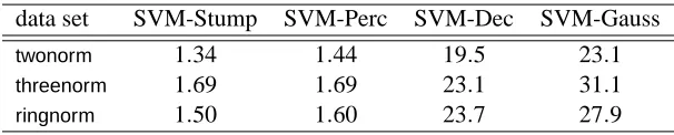
Second, we can group kernels by whether they are scale-invariant (see also Section 5). The sim-plified stump kernel and the simsim-plified perceptron kernel are scale-invariant, which means that C is the only parameter that needs to be determined. On the other hand, different combinations of(γ,C) need to be considered for the Gaussian-RBF kernel or the Laplacian-RBF kernel during parameter selection (Keerthi and Lin, 2003). Thus, SVM with the simplified stump kernel or the simpli-fied perceptron kernel enjoys an advantage on speed during parameter selection. As we will see in Section 7.2, experimentally they perform similarly to the Gaussian-RBF kernel on many data sets. Thus, SVM applications that consider speed as an important factor may benefit from using the simplified stump kernel or the simplified perceptron kernel.

7. Experiments

We first compare our SVM-based infinite ensemble learning framework with AdaBoost and LP-Boost using decision stumps, perceptrons, or decision trees as the base hypothesis set. The simpli-fied stump kernel (SVM-Stump), the simplisimpli-fied perceptron kernel (SVM-Perc), and the Laplacian-RBF kernel (SVM-Dec) are plugged into Algorithm 1 respectively. We also compare SVM-Stump, SVM-Perc, and SVM-Dec with SVM-Gauss, which is SVM with the Gaussian-RBF kernel.

The deterministic decision stump algorithm (Holte, 1993), the random coordinate descent per-ceptron algorithm (Li and Lin, 2007), and the C4.5 decision tree algorithm (Quinlan, 1986) are taken as base learners in AdaBoost and LPBoost for the corresponding base hypothesis set. For perceptrons, we use the RCD-bias setting with 200 epochs of training; for decision trees, we take the pruned tree with the default settings of C4.5. All base learners above have been shown to work reasonably well with boosting in literature (Freund and Schapire, 1996; Li and Lin, 2007).

We discussed in Subsection 4.2 that a common implementation of AdaBoost-Stump and LPBoost-Stump only chooses the middle stumps. For further comparison, we include all the middle stumps in a set

M

, and construct a kernel

K

_M with r= 1

2 according to Definition 1. Because

M

is a finite set, the integral in (4) becomes a summation when computed with the counting measure. We test our framework with this kernel, and call it SVM-Mid.

LIBSVM 2.8 (Chang and Lin, 2001a) is adopted as the soft-margin SVM solver, with a sug-gested procedure that selects a suitable parameter with a five-fold cross validation on the training set (Hsu et al., 2003). For SVM-Stump, SVM-Mid, and SVM-Perc, the parameter log₂C is searched within_{−17,₋15, . . . ,3_}, and for SVM-Dec and SVM-Gauss, the parameters (log₂γ,log₂C) are searched within _{−15,₋13, . . . ,3_{} × {−}5,₋3, . . . ,15_}. We use different search ranges for log₂C because the numerical ranges of the kernels could be quite different. After the parameter selection procedure, a new model is trained using the whole training set, and the generalization ability is evaluated on an unseen test set.

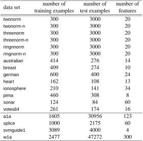
data set number of number of number of training examples test examples features

twonorm 300 3000 20

twonorm-n 300 3000 20

threenorm 300 3000 20

threenorm-n 300 3000 20

ringnnorm 300 3000 20

ringnorm-n 300 3000 20

australian 414 276 14

breast 409 274 10

german 600 400 24

heart 162 108 13

ionosphere 210 141 34

pima 460 308 8

sonar 124 84 60

votes84 261 174 16

a1a 1605 30956 123

splice 1000 2175 60

svmguide1 3089 4000 4

w1a 2477 47272 300

Table 1: Summarized information of the data sets used

is searched within _{10,20, . . . ,1500_}. Note that because LPBoost can be slow when the ensem-ble size is too large (Demiriz et al., 2002), we set a stopping criterion to generate at most 1000 columns (hypotheses) in order to obtain an ensemble within a reasonable amount of time.

The three artificial data sets from Breiman (1999) (twonorm,threenorm, andringnorm) are gen-erated with training set size 300 and test set size 3000. We create three more data sets (twonorm-n,

threenorm-n,ringnorm-n), which contain mislabeling noise on 10% of the training examples, to test the performance of the algorithms on noisy data. We also use eight real-world data sets from the UCI repository (Hettich et al., 1998): australian,breast, german,heart,ionosphere,pima, sonar, and

votes84. Their feature elements are scaled to[₋1, 1]. We randomly pick 60% of the examples for training, and the rest for testing. For the data sets above, we compute the means and the standard errors of the results over 100 runs. In addition, four larger real-world data sets are used to test the validity of the framework for large-scale learning. They area1a(Hettich et al., 1998; Platt, 1999),

splice (Hettich et al., 1998), svmguide1(Hsu et al., 2003), and w1a (Platt, 1999).6 Each of them comes with a benchmark test set, on which we report the results. Some information of the data sets used is summarized in Table 1.

data set SVM-Stump SVM-Mid AdaBoost-Stump LPBoost-Stump

twonorm 2.86_±0.04 3.10_±0.04 5.02_±0.06 5.58_±0.07

twonorm-n 3.08_±0.06 3.29_±0.05 12.7_±0.17 17.9_±0.19

threenorm 17.7_±0.10 18.6_±0.12 22.1_±0.12 24.1_±0.15

threenorm-n 19.0_±0.14 19.6_±0.13 26.1_±0.17 30.3_±0.16

ringnorm 3.97_±0.07 5.30_±0.07 10.1_±0.14 10.3_±0.14

ringnorm-n 5.56_±0.11 7.03_±0.14 19.6_±0.20 22.4_±0.21

australian 14.4_±0.21 15.9_±0.18 14.2_±0.18 19.8_±0.24

breast 3.11±0.08 2.77±0.08 4.41±0.10 4.79±0.12

german 24.7_±0.18 24.9_±0.17 25.4_±0.19 31.6_±0.20

heart 16.4_±0.27 19.1_±0.35 19.2_±0.35 24.4_±0.39

ionosphere 8.13±0.17 8.37±0.20 11.3±0.25 11.5±0.24

pima 24.1_±0.23 24.4_±0.23 24.8_±0.23 31.0_±0.24

sonar 16.6_±0.42 18.0_±0.37 19.4_±0.38 19.8_±0.37

votes84 4.76±0.14 4.76±0.14 4.27±0.15 5.87±0.16

a1a 16.2 16.3 16.0 16.3

splice 6.21 6.71 5.75 8.78

svmguide1 2.92 3.20 3.35 4.50

w1a 2.09 2.26 2.18 2.79

Table 2: Test error (%) of several ensemble learning algorithms using decision stumps

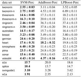
data set SVM-Perc AdaBoost-Perc LPBoost-Perc

twonorm 2.55_±0.03 3.11_±0.04 3.52_±0.05

twonorm-n 2.75_±0.05 4.53_±0.10 6.89_±0.11

threenorm 14.6_±0.08 17.3_±0.11 18.2_±0.11

threenorm-n 16.3_±0.10 20.0_±0.18 22.1_±0.13

ringnorm 2.46_±0.04 36.3_±0.14 37.4_±0.13

ringnorm-n 3.50_±0.09 37.8_±0.20 39.1_±0.15

australian 14.5_±0.17 15.7_±0.16 16.4_±0.17

breast 3.23±0.08 3.49±0.10 3.80±0.10

german 24.6_±0.20 25.0_±0.18 26.4_±0.21

heart 17.6_±0.31 18.2_±0.32 19.8_±0.32

ionosphere 6.40±0.20 11.4±0.23 12.1±0.25

pima 23.5_±0.21 24.8_±0.20 26.4_±0.19

sonar 15.6_±0.40 19.8_±0.43 22.5_±0.47

votes84 4.43±0.14 4.37±0.16 4.92±0.16

a1a 15.7 20.0 18.6

splice 10.4 13.7 14.7

svmguide1 3.10 3.28 3.62

w1a 1.91 2.35 2.13

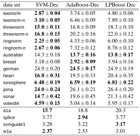
data set SVM-Dec AdaBoost-Dec LPBoost-Dec

twonorm 2.87_±0.04 3.74_±0.05 4.80_±0.06

twonorm-n 3.10_±0.05 6.46_±0.09 7.89_±0.10

threenorm 15.0_±0.11 16.8_±0.09 18.3_±0.10

threenorm-n 16.8_±0.15 20.2_±0.16 22.0_±0.12

ringnorm 2.25_±0.05 4.33_±0.06 6.00_±0.10

ringnorm-n 2.67_±0.06 7.32_±0.12 8.76_±0.12

australian 14.3_±0.18 13.7_±0.16 13.8_±0.17

breast 3.18_±0.08 2.92_±0.09 3.94_±0.16

german 24.9_±0.20 24.5_±0.17 24.9_±0.19

heart 16.8_±0.31 19.5_±0.33 20.4_±0.35

ionosphere 6.48_±0.19 6.59_±0.19 6.81_±0.22

pima 24.0_±0.24 26.1_±0.21 26.4_±0.20

sonar 14.7_±0.42 19.6_±0.45 21.3_±0.42

votes84 4.59_±0.15 5.04_±0.14 5.95_±0.17

a1a 15.7 18.8 20.3

splice 3.77 2.94 3.77

svmguide1 3.28 3.22 3.17

w1a 2.37 2.53 3.01

Table 4: Test error (%) of several ensemble learning algorithms using decision trees

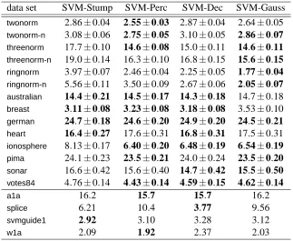
7.1 Comparison of Ensemble Learning Algorithms

Tables 2, 3, and 4 show the test performance of several ensemble learning algorithms on different base hypothesis sets.7 We can see that SVM-Stump, SVM-Perc, and SVM-Dec are usually better than AdaBoost and LPBoost with the same base hypothesis set, especially for the cases of decision stumps and perceptrons. In noisy data sets, SVM-based infinite ensemble learning always signifi-cantly outperforms AdaBoost and LPBoost. These results demonstrate that it is beneficial to go from a finite ensemble to an infinite one with suitable regularization. When comparing the two boosting approaches, LPBoost is at best comparable to AdaBoost on a small number of the data sets, which suggests that the success of AdaBoost may not be fully attributed to its connection to(P3)or(P4).

Note that SVM-Stump, SVM-Mid, AdaBoost-Stump, and LPBoost-Stump usually generate dif-ferent kinds of ensembles: SVM-Stump produces infinite and nonsparse ones; SVM-Mid produces finite and nonsparse ones; AdaBoost-Stump produces finite and sparse ones; LPBoost-Stump pro-duces finite and even sparser ones (since some of the selected ht may end up having wt =0). In

Ta-ble 2, we see that SVM-Stump often outperforms SVM-Mid, which is another evidence that an infinite ensemble could help. Interestingly, SVM-Mid often performs better than AdaBoost-Stump, which means that a nonsparse ensemble introduced by minimizing the`2-norm of w is better than a sparse one.

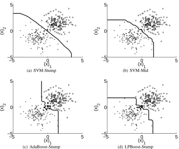
In Figure 3, we further illustrate the difference between the finite and infinite ensemble learning algorithms by a simplified experiment. We show the decision boundaries generated by the four algorithms on 300 training examples from the 2-D version of the twonorm data set. The

−5 0 5 −5

0 5

(x) 1

(x)

2

(a) SVM-Stump

−5 0 5

−5 0 5

(x) 1

(x)

2

(b) SVM-Mid

−5 0 5

−5 0 5

(x) 1

(x)

2

(c) AdaBoost-Stump

−5 0 5

−5 0 5

(x) 1

(x)

2

(d) LPBoost-Stump

Figure 3: Decision boundaries of ensemble learning algorithms on a 2-Dtwonormdata set

optimal decision boundary is the line (x)1+ (x)2=0. We can see that SVM-Stump produces a decision boundary close to the optimal, SVM-Mid is slightly worse, while AdaBoost-Stump and LPBoost-Stump fail to generate a decent boundary. SVM-Stump obtains the smooth boundary by averaging over infinitely many decision stumps; SVM-Mid can also generate a smooth boundary by constructing a nonsparse ensemble over a finite number of decision stumps. Nevertheless, both LPBoost-Stump and AdaBoost-Stump, for which sparsity could be observed from the axis-parallel decision boundaries, do not have the ability to approximate the Bayes optimal boundary well. In addition, as can be seen near the origin point of Figure 3(c), AdaBoost-Stump could suffer from overfitting the noise.