Efficient Online and Batch Learning Using
Forward Backward Splitting
John Duchi [email protected]
Computer Science Division University of California, Berkeley Berkeley, CA 94720 USA
Yoram Singer [email protected]
1600 Amphitheatre Pkwy Mountain View, CA 94043 USA
Editor: Yoav Freund
Abstract
We describe, analyze, and experiment with a framework for empirical loss minimization with regularization. Our algorithmic framework alternates between two phases. On each iteration we first perform an uncon-strained gradient descent step. We then cast and solve an instantaneous optimization problem that trades off minimization of a regularization term while keeping close proximity to the result of the first phase. This view yields a simple yet effective algorithm that can be used for batch penalized risk minimization and on-line learning. Furthermore, the two phase approach enables sparse solutions when used in conjunction with regularization functions that promote sparsity, such asℓ1. We derive concrete and very simple algorithms for minimization of loss functions withℓ1,ℓ2,ℓ2
2, andℓ∞ regularization. We also show how to construct ef-ficient algorithms for mixed-normℓ1/ℓqregularization. We further extend the algorithms and give efficient
implementations for very high-dimensional data with sparsity. We demonstrate the potential of the proposed framework in a series of experiments with synthetic and natural data sets.
Keywords: subgradient methods, group sparsity, online learning, convex optimization
1. Introduction
Before we begin, we establish notation for the content of this paper. We denote scalars by lower case letters and vectors by lower case bold letters, for example,w. The inner product of two vectorsuandvis denoted
hu,vi. We usekxkpto denote the p-norm of the vectorxandkxkas a shorthand forkxk2.
The focus of this paper is an algorithmic framework for regularized convex programming to minimize the following sum of two functions:
f(w) +r(w), (1)
where both f and r are convex bounded below functions (so without loss of generality we assume they are intoR+). Often, the function f is an empirical loss and takes the form ∑i∈Sℓi(w)for a sequence of loss functionsℓi:Rn→R+, and r(w)is a regularization term that penalizes for excessively complex vectors, for instance r(w) =λkwkp. This task is prevalent in machine learning, in which a learning problem for decision
and prediction problems is cast as a convex optimization problem. To that end, we investigate a general and intuitive algorithm, known as forward-backward splitting, to minimize Eq. (1), focusing especially on derivations for and use of non-differentiable regularization functions.
Many methods have been proposed to minimize general convex functions such as that in Eq. (1). One of the most general is the subgradient method (see, e.g., Bertsekas, 1999), which is elegant and very simple. Let
∂f(w)denote the subgradient set of f atw, namely,
Sub-gradient procedures then minimize the function f(w)by iteratively updating the parameter vectorw according to the update rule
wt+1=wt−ηtgtf ,
whereηtis a constant or diminishing a step size andgtf ∈∂f(wt)is an arbitrary vector from the subgradient
set of f evaluated atwt. A more general method than the above is the projected gradient method, which
iterates
wt+1 = ΠΩ
wt−ηtgtf
= argmin
w∈Ω
w−(wt−ηtg
f t)
2
2
whereΠΩ(w)is the Euclidean projection ofwonto the setΩ. Standard results (Bertsekas, 1999) show that the (projected) subgradient method converges at a rate of O(1/ε2), or equivalently that the error f(
w)− f(w⋆) =O(1/√T), given some simple assumptions on the boundedness of the subdifferential set andΩ(we have omitted constants dependent onk∂fkor dim(Ω)).
If we use the subgradient method to minimize Eq. (1), the iterates are simplywt+1=wt−ηtgtf−ηtgtr, wheregtr∈∂r(wt). A common problem in subgradient methods is that if r or f is non-differentiable, the
iterates of the subgradient method are very rarely at the points of non-differentiability. In the case of regu-larization functions such as r(w) =kwk1, however, these points (zeros in the case of theℓ1-norm) are often
the true minima of the function. Furthermore, withℓ1and similar penalties, zeros are desirable solutions as
they tend to convey information about the structure of the problem being solved, and in the case of statistical inference, can often yield the correct sparsity structure of the parameters (Zhao and Yu, 2006; Meinshausen and B¨uhlmann, 2006).
There has been a significant amount of work related to minimizing Eq. (1), especially when the func-tion r is a sparsity-promoting regularizer, and much of it stems from the machine learning, statistics, and optimization communities. We can hardly do justice to the body of prior work, and we provide a few refer-ences here to the research we believe is most directly related. The approach we pursue below is known as forward-backward splitting in the optimization literature, which is closely related to the proximal method.
The forward-backward splitting method was first proposed by Lions and Mercier (1979) and has been ana-lyzed by several researches in the context of maximal monotone operators in the optimization literature. Chen and Rockafellar (1997) and Tseng (2000) give conditions and modifications of forward-backward splitting to attain linear convergence rates. Combettes and Wajs (2005) give proofs of convergence for forward-backward splitting in Hilbert spaces under asymptotically negligible perturbations, though without establishing strong rates of convergence. Prior work on convergence of the method often requires an assumption of strong mono-tonicity of the maximal monotone operators (equivalent to strong convexity of at least one of the functions in Eq. (1)), and as far as we know, all analyses assume that f is differentiable with Lipschitz-continuous gradient. The analyses have also been carried out in a non-stochastic and non-online setting.
More recently, Wright et al. (2009) suggested the use of the method for sparse signal reconstruction, where f(w) =ky−Awk2, though they note that the method can apply to suitably smooth convex functions f . Nesterov (2007) gives analysis of convergence rates using gradient mapping techniques when f has Lipschitz continuous gradient, which was inspired by Wright et al. In the special case that r(w) =λkwk1, similar methods to the algorithms we investigate have been proposed and termed iterative thresholding (Daubechies et al., 2004) or truncated gradient (Langford et al., 2008) in signal processing and machine learning, but the authors were apparently unaware of the connection to splitting methods.
Similar projected-gradient methods, when the regularization function r is no longer part of the objective function but rather cast as a constraint so that r(w)≤λ, are also well known (Bertsekas, 1999). In signal processing, the problem is often termed as an inverse problem with sparsity constraints, see for example, Daubechies et al. (2008) and the references therein. Duchi et al. (2008) give a general and efficient projected gradient method forℓ1-constrained problems. We make use of one of Duchi et al.’s results in obtaining
the context of consistency and recovery of sparsity patterns throughℓ1or mixed-norm regularization across
multiple tasks (Meinshausen and B¨uhlmann, 2006; Obozinski et al., 2008; Zhao et al., 2006).
In this paper, we describe a general gradient-based framework for online and batch convex programming. To make our presentation a little simpler, we call our approach FOBOS, for FOrward-Backward Splitting.1 Our proofs are made possible through the use of “forward-looking” subgradients, and FOBOSis a distillation of some the approaches mentioned above for convex programming. Our alternative view lends itself to unified analysis and more general settings, efficient implementation, and provides a flexible tool for the derivation of algorithms for old and new convex programming settings.
The paper is organized as follows. In the next section, we begin by introducing and formally defining the method, giving some simple preliminary analysis. We follow the introduction by giving in Sec. 3 rates of convergence for batch (offline) optimization. We then extend the results to stochastic gradient descent and provide regret bounds for online convex programming in Sec. 4. To demonstrate the simplicity and usefulness of the framework, we derive in Sec. 5 algorithms for several different choices of the regularizing function r, though most of these results are known. We then extend these methods to be efficient in very high dimensional learning settings where the input data is sparse in Sec. 6. Finally, we conclude in Sec. 7 with experiments examining various aspects of the proposed framework, in particular the runtime and sparsity selection performance of the derived algorithms.
2. Forward-Looking Subgradients and Forward-Backward Splitting
Our approach to Forward-Backward Splitting is motivated by the desire to have the iterateswt attain points
of non-differentiability of the function r. The method alleviates the problems of non-differentiability in cases such as ℓ1-regularization by taking analytical minimization steps interleaved with subgradient steps.
Put informally, FOBOScan be viewed as analogous to the projected subgradient method while replacing or augmenting the projection step with an instantaneous minimization problem for which it is possible to derive a closed form solution. FOBOSis succinct as each iteration consists of the following two steps:
wt+1
2 = wt−ηtg
f
t, (2)
wt+1 = argmin w
1 2
w−wt+12
2 +ηt+1
2
r(w)
. (3)
In the above,gtf is a vector in∂f(wt)andηtis the step size at time step t of the algorithm. The actual value
ofηt depends on the specific setting and analysis. The first step thus simply amounts to an unconstrained
subgradient step with respect to the function f . In the second step we find a new vector that interpolates between two goals: (i) stay close to the interim vector wt+1
2, and (ii) attain a low complexity value as expressed by r. Note that the regularization function is scaled by an interim step size, denotedηt+1
2. The analyses we describe in the sequel determine the specific value ofηt+1
2, which is eitherηtorηt+1.
A key property of the solution of Eq. (3) is the necessary condition for optimality and gives the reason behind the name FOBOS. Namely, the zero vector must belong to subgradient set of the objective at the optimumwt+1, that is,
0∈∂ 1
2
w−wt+1 2
2 +ηt+1
2r(w)
w=wt+1 .
Sincewt+1
2 =wt−ηtg
f
t, the above property amounts to
0∈wt+1−wt+ηtgf
t +ηt+1
2∂r(wt+1). (4)
The property0∈wt+1−wt+ηtgf
t +ηt+1
2∂r(wt+1)implies that so long as we choosewt+1to be the mini-mizer of Eq. (3), we are guaranteed to obtain a vectorgtr+1∈∂r(wt+1)such that
0=wt+1−wt+ηtgtf+η
t+1
2g
r t+1 .
The above equation can be understood as an update scheme where the new weight vectorwt+1is a linear
combination of the previous weight vectorwt, a vector from the subgradient set of f evaluated atwt, and a
vector from the subgradient of r evaluated at the yet to be determinedwt+1, hence the name Forward-Looking
Subgradient. To recap, we can writewt+1as
wt+1=wt−ηtgtf−ηt+12g
r
t+1, (5)
wheregtf ∈∂f(wt)andgtr+1∈∂r(wt+1). Solving Eq. (3) with r above has two main benefits. First, from an algorithmic standpoint, it enables sparse solutions at virtually no additional computational cost. Second, the forward-looking gradient allows us to build on existing analyses and show that the resulting framework enjoys the formal convergence properties of many existing gradient-based and online convex programming algorithms.
3. Convergence Analysis of FOBOS
Upon first look FOBOSlooks substantially different from sub-gradient and online convex programming meth-ods. However, the fact that FOBOS actually employs a forward-looking subgradient of the regularization function lets us build nicely on existing analyses. In this section we modify known results while using the forward-looking property of FOBOSto provide convergence rate analysis for FOBOS. To do so we will set
ηt+1
2 properly. As we show in the sequel, it is sufficient to setηt+12 toηt orηt+1, depending on whether we are doing online or batch optimization, in order to obtain convergence and low regret bounds. We start with an analysis of FOBOSin a batch setting. In this setting we use the subgradient of f , setηt+1
2 =ηt+1and
updatewttowt+1as prescribed by Eq. (2) and Eq. (3).
Throughout the section we denote by w⋆ the minimizer of f(w) +r(w). In what follows, define
k∂f(w)k,supg∈∂f(w)kgk. We begin by deriving convergence results under the fairly general
assump-tion (see, e.g., Langford et al. 2008 or Shalev-Shwartz and Tewari 2009) that the subgradients are bounded as follows:
k∂f(w)k2≤A f(w) +G2, k∂r(w)k2≤Ar(w) +G2 . (6)
For example, any Lipschitz loss (such as the logistic loss or hinge loss used in support vector machines) satisfies the above with A=0 and G equal to the Lipschitz constant. Least squares estimation satisfies Eq. (6) with G=0 and A=4. The next lemma, while technical, provides a key tool for deriving all of the convergence results in this paper.
Lemma 1 (Bounding Step Differences) Assume that the norms of the subgradients of the functions f and r are bounded as in Eq. (6):
k∂f(w)k2≤A f(w) +G2, k∂r(w)k2≤Ar(w) +G2 .
Letηt+1≤ηt+1
2 ≤ηtand suppose thatηt≤2ηt+12. If we use the FOBOSupdate of Eqs. (2) and (3), then for
a constant c≤4 and any vectorw⋆,
2ηt(1−cAηt)f(wt) +2ηt+1
2(1−cAηt+12)r(wt+1)
≤ 2ηtf(w⋆) +2ηt+1
2r(w
⋆) +k
wt−w⋆k2− kwt+1−w⋆k2+7ηtηt+1
2G
Proof We begin with a few simple properties of the forward-looking subgradient steps before proceeding
with the core of the proof. Note first that for somegtf ∈∂f(wt)andgrt+1∈∂r(wt+1), we have as in Eq. (5)
wt+1−wt=−ηtgtf−ηt+1
2g
r
t+1 . (7)
The definition of a subgradient implies that for anygtr+1∈∂r(wt+1)(and similarly for anygtf∈∂f(wt)with
f(wt)and f(w⋆))
r(w⋆)≥r(wt+1) +gtr+1,w⋆−wt+1 ⇒ −gtr+1,wt+1−w⋆≤r(w⋆)−r(wt+1). (8)
From the Cauchy-Shwartz Inequality and Eq. (7), we obtain
gtr+1,(wt+1−wt) =
D
gtr+1,(−ηtgtf−ηt+1
2g
r t+1)
E
≤ kgtr+1kkηt+1
2g
r
t+1+ηtgtfk ≤ ηt+1
2kg
r
t+1k2+ηtkgtr+1kkgtfk
≤ ηt+12 Ar(wt+1) +G
2
+ηt A max{f(wt),r(wt+1)}+G2 . (9)
We now proceed to bound the difference betweenw⋆andwt+1, and using a telescoping sum we will
even-tually bound f(wt) +r(wt)−f(w⋆)−r(w⋆). First, we expand norm squared of the difference betweenwt
andwt+1,
kwt+1−w⋆k2 = kwt−(ηtgtf+ηt+1
2g
r
t+1)−w⋆k2
= kwt−w⋆k2−2 h
ηt
D
gtf,wt−w⋆ E
+ηt+1 2
gtr+1,wt−w⋆ i
+kηtgtf+ηt+1
2g
r t+1k2
= kwt−w⋆k2−2ηt
D
gtf,wt−w⋆ E
+kηtgtf+ηt+1
2g
r t+1k2
−2ηt+1 2
gtr+1,wt+1−w⋆−gtr+1,wt+1−wt . (10)
We can bound the third term above by noting that
kηtgtf+ηt+1
2g
r t+1k2
= η2
tkgtfk2+2ηtηt+1 2
D gtf,gtr+1
E
+η2
t+12kg
r t+1k2
≤ η2
tA f(wt) +2ηtηt+1
2A max{f(wt),r(wt+1)}+η
2
t+12A r(wt+1) +4η 2
tG2 .
We now use Eq. (9) to bound the last term of Eq. (10) and the above bound onηtgtf+ηt+12gtr+1to get that
kwt+1−w⋆k2
≤ kwt−w⋆k2−2ηt
D
gtf,wt−w⋆ E
−2ηt+1 2
gtr+1,wt+1−w⋆+kηtgtf+ηt+1
2g
r t+1k2
+2ηt+1 2
ηt+1
2A r(wt+1) +2ηtA max{f(wt),r(wt+1)}+2ηtG
2
≤ kwt−w⋆k2+2ηt(f(w⋆)−f(wt)) +2ηt+1
2(r(w
⋆)−r(
wt)) +7η2tG2
+η2tA f(wt) +3ηtηt+1
2A max{f(wt),r(wt)}+2η
2
t+1 2
A r(wt+1) (11)
≤ kwt−w⋆k2+7η2tG2
+2ηt(f(w⋆)−(1−cηtA)f(wt)) +2ηt+1 2
r(w⋆)−(1−cηt+1
2A)r(wt+1)
. (12)
To obtain Eq. (11) we used the standard convexity bounds established earlier in Eq. (8). The final bound given by Eq. (12) is due to the fact that 3Aηtηt+1
2 ≤6Aη
2
the terms f(·)and r(·)yields the desired inequality.
The lemma allows a proof of the following theorem, which constitutes the basis for deriving concrete convergence results for FOBOS. It is also demonstrates the ease of proving convergence results based on the lemma and the forward looking property.
Theorem 2 Assume the following hold: (i) the norm of any subgradient from∂f and the norm of any
sub-gradient from∂r are bounded as in Eq. (6), (ii) the norm ofw⋆is less than or equal to D, (iii) r(0) =0, and
(iv)12ηt≤ηt+1≤ηt. Then for a constant c≤4 withw1=0andηt+1
2 =ηt+1,
T
∑
t=1
[ηt((1−cAηt)f(wt)−f(w⋆)) +ηt((1−cAηt)r(wt)−r(w⋆))]≤D2+7G2
T
∑
t=1
η2
t .
Proof Rearranging the f(w⋆)and r(w⋆)terms from the bound in Lemma 1, we sum the loss terms over t from 1 through T and get a canceling telescoping sum:
T
∑
t=1
[ηt((1−cAηt)f(wt)−f(w⋆)) +ηt+1((1−cAηt+1)r(wt+1)−r(w⋆))]
≤ kw1−w⋆k2− kwT+1−w⋆k2+7G2
T
∑
t=1
η2
t ≤ kw1−w⋆k2+7G2
T
∑
t=1
η2
t . (13)
We now bound the time-shifted r(wt+1)terms by noting that
T
∑
t=1
ηt+1((1−cAηt+1)r(wt+1)−r(w⋆))
=
T
∑
t=1
ηt((1−cAηt)r(wt)−r(w⋆)) +ηT+1((1−cAηT+1)r(wt+1)−r(w⋆)) +η1r(w⋆)
≥
T
∑
t=1
ηt((1−cAηt)r(wt+1)−r(w⋆)) +r(w⋆)(η1−ηT+1)
≥
T
∑
t=1
ηt((1−cAηt)r(wt)−r(w⋆)) . (14)
Finally, we use the fact thatkw1−w⋆k=kw⋆k ≤D, along with with Eq. (13)) and Eq. (14) to get the desired bound.
In the remainder of this section, we present a few corollaries that are consequences of the theorem. The first corollary underscores that the rate of convergence in general is approximately 1/ε2, or, equivalently,
1/√T .
Corollary 3 (Fixed step rate) Assume that the conditions of Thm. 2 hold and that we run FOBOS for a
predefined T iterations withηt=√7T GD and that(1−cA√7T GD )>0. Then
min
t∈{1,...,T}f(wt) +r(wt)≤
1 T
T
∑
t=1
f(wt) +r(wt)≤
3DG
√
T1− cAD
G√7T
+
f(w⋆) +r(w⋆)
1− cAD
Proof Since we haveηt=ηfor all t, the bound on the convergence rate from Thm. 2 becomes
η(1−cAη)T min
t∈{1,...,T}[f(wt) +r(wt)−f(w
⋆)−r(
w⋆)]
≤ η(1−cAη)
T
∑
t=1
[f(wt)−f(w⋆)] + [r(wt)−r(w⋆)] ≤ D2+7G2Tη2 .
Plugging in the specified value forηgives the bound.
Another direct consequence of Thm. 2 is convergence of the minimum over t when running FOBOSwith
ηt∝1/√t or with non-summable step sizes decreasing to zero.
Corollary 4 (Convergence of decreasing step sizes) Assume that the conditions of Thm. 2 hold and the step
sizesηtsatisfyηt→0 and∑∞t=1ηt=∞. Then
lim inf
t→∞ f(wt) +r(wt)−(f(w
⋆) +r(
w⋆)) =0.
Finally, when f and r are Lipschitz with Lipschitz constant G, we immediately have
Corollary 5 In addition to the conditions of Thm. 2, assume that the norm of any subgradient from∂f and
the norm of any subgradient from∂r are bounded by G. Then
min
t∈{1,...,T}(f(wt) +r(wt))−(f(w
⋆) +r(
w⋆))≤D
2+7G2∑T t=1η2t
2∑Tt=1ηt
. (15)
Bounds of the above form, where we obtain convergence for one of the points in the sequencew1, . . . ,wT
rather than the last pointwT, are standard in subgradient optimization. The main reason that this weaker result
occurs is due to the fact that we cannot guarantee a strict descent direction when using arbitrary subgradients (see, for example, Theorem 3.2.2 from Nesterov 2004). Another consequence of using non-differentiable functions means that analyses such as those carried out by Tseng (2000) and Chen and Rockafellar (1997) are difficult to apply, as the stronger rates rely on the existence and Lipschitz continuity of∇f(w). However, it is possible to show linear convergence rates under suitable smoothness and strong convexity assumptions. When∇f(w)is Lipschitz continuous, a more detailed analysis yields convergence rates of 1/ε(namely, 1/T in terms of number of iterations needed to beεclose to the optimum). A more complicated algorithm related to Nesterov’s “estimate functions” (Nesterov, 2004) leads to O(1/√ε)convergence (Nesterov, 2007). For completeness, we give a simple proof of 1/T convergence in Appendix C. Finally, the above proof can be modified slightly to give convergence of the stochastic gradient method. In particular, we can replacegtf in
the iterates of FOBOSwith a stochastic estimate of the gradient ˜gtf, where E[g˜tf]∈∂f(wt). We explore this
approach in slightly more depth after performing a regret analysis for FOBOSbelow in Sec. 4 and describe stochastic convergence rates in Corollary 10.
We would like to make further comments on our proof of convergence for FOBOSand the assumptions underlying the proof. It is often not necessary to have a Lipschitz loss to guarantee boundedness of the subgradients of f and r, so in practice an assumption of bounded subgradients (as in Corollary 5 and in the sequel for online analysis) is not restrictive. If we know that an optimalw⋆lies in some compact setΩand thatΩ⊆dom(f+r), then Theorem 24.7 of Rockafellar (1970) guarantees that∂f and∂r are bounded. The lingering question is thus whether we can guarantee that such a setΩexists and that our iterateswt remain
inΩ. The following simple setting shows that∂f and∂r are indeed often bounded.
If r(w)is a norm (possibly scaled) and f is lower bounded by 0, then we know that r(w⋆)≤ f(w⋆) + r(w⋆)≤f(w1) +r(w1). Using standard bounds on norms, we get that for someγ>0
where for the last inequality we used the assumption that r(w1) =0. Thus, we obtain that w⋆ lies in a hypercube. We can easily project onto this box by truncating elements ofwt lying outside it at any iteration
without affecting the bounds in Eq. (12) or Eq. (15). This additional Euclidean projectionΠΩto an arbitrary convex setΩwithw⋆∈Ω satisfieskΠΩ(wt+1)−w⋆k ≤ kwt+1−w⋆k. Furthermore, so long asΩ is an ℓp-norm ball, we know that
r(ΠΩ(wt+1))≤r(wt+1) . (16)
Thus, looking at Eq. (11), we notice that r(w⋆)−r(wt+1)≤r(w⋆)−r(ΠΩ(wt+1))and the series of inequal-ities through Eq. (12) still hold (so long as cηt+1
2
A≤1, which it will ifΩis compact so that we can take A=0). In general, so long as Eq. (16) holds andw⋆∈Ω, we can projectwt+1 intoΩ without affecting
convergence guarantees. This property proves to be helpful in the regret analysis below.
4. Regret Analysis of FOBOS
In this section we provide regret analysis for FOBOSin online settings. In an online learning problem, we are given a sequence of functions ft:Rn→R. The learning goal is for the sequence of predictionswt
to attain low regret when compared to a single optimal predictorw⋆. Formally, let ft(w)denote the loss suffered on the tth input loss function when using a predictorw. The regret of an online algorithm which usesw1, . . . ,wt, . . .as its predictors w.r.t. a fixed predictorw⋆while using a regularization function r is
Rf+r(T) =
T
∑
t=1
[ft(wt) +r(wt)−(ft(w⋆) +r(w⋆))].
Ideally, we would like to achieve 0 regret to a stationaryw⋆for arbitrary length sequences.
To achieve an online bound for a sequence of convex functions ft, we modify arguments of Zinkevich
(2003). Using the bound from Lemma 1, we can readily state and prove a theorem on the online regret of FOBOS. It is possible to avoid the boundedness assumptions in the proof of the theorem (getting a bound similar to that of Theorem 2 but for regret), however, we do not find it significantly more interesting. Aside from its reliance on Lemma 1, this proof is quite similar to Zinkevich’s, so we defer it to Appendix A.
Theorem 6 Assume thatkwt−w⋆k ≤D for all iterations and the norm of the subgradient sets∂ft and∂r
are bounded above by G. Let c>0 an arbitrary scalar. Then, the regret bound of FOBOSwithηt=c/√t
satisfies
Rf+r(T)≤2GD+
D2
2c+7G
2c
√
T .
The following Corollary is immediate from Theorem 6.
Corollary 7 Assume the conditions of Theorem 6 hold. Then, settingηt=4GD√t, the regret of FOBOSis
Rf+r(T)≤2GD+4GD
√
T .
We can also obtain a better regret bound for FOBOS when the sequence of loss functions ft(·)or the
function r(·)is strongly convex. As demonstrated by Hazan et al. (2006), with the projected gradient method and strongly convex functions, it is possible to achieve regret on the order of O(log T)by using the curvature of the sequence of functions ftrather than simply using convexity and linearity as in Theorems 2 and 6. We
can extend these results to FOBOSfor the case in which ft(w) +r(w)is strongly convex, at least over the domainkw−w⋆k ≤D. For completeness, we recap a few definitions and provide the logarithmic regret bound for FOBOS. A function f is called H-strongly convex if
f(w)≥f(wt) +h∇f(wt),w−wti+
H
2kw−wtk
Thus, if r and the sequence of functions ftare strongly convex with constants Hf ≥0 and Hr≥0, we have
H=Hf+Hrand H-strong convexity gives
ft(wt)−f(w⋆) +r(wt)−r(w⋆)≤
D
gtf+gtr,wt−w⋆ E
−H2kwt−w⋆k2 . (17)
We do not need to assume that both ft and r are strongly convex. We only need assume that at least one of
them attains a positive strong convexity constant. For example, if r(w) = λ2kwk2, then H≥λso long as the functions ftare convex. With Eq. (17) in mind, we can readily build on Hazan et al. (2006) and prove a
stronger regret bound for the online learning case. The proof is similar to that of Hazan et al., so we defer it also to Appendix A.
Theorem 8 Assume as in Theorem 6 thatkwt−w⋆k ≤D and that∂ft and ∂r are bounded above by G.
Assume further that ft+r is H-strongly convex for all t. Then, when using step sizesηt=1/Ht, the regret of
FOBOSis
Rf+r(T) =O
G2
H log T
.
We now provide an easy lemma showing that for Lipschitz losses withℓ2
2regularization, the boundedness
assumptions above hold. This, for example, includes the interesting case of support vector machines. The proof is not difficult but relies tacitly on a later result, so we leave it to Appendix A.
Lemma 9 Let the functions ftbe G-Lipschitz so thatk∂ft(w)k ≤G. Let r(w) =λ2kwk2. Thenkw⋆k ≤G/λ
and the iterateswtgenerated by FOBOSsatisfykwtk ≤G/λ.
Using the regret analysis for online learning, we are able to return to learning in a batch setting and give stochastic convergence rates for FOBOS. We build on results of Shalev-Shwartz et al. (2007) and assume as in Sec. 3 that we are minimizing f(w) +r(w). Indeed, suppose that on each step of FOBOS, we choose instead of somegtf ∈∂f(wt)a stochastic estimate of the gradient ˜gtf where E[g˜tf]∈∂f(wt). We assume that we still
use the true r (which is generally easy, as it is simply the regularization function). It is straightforward to use theorems 6 and 8 above as in the derivation of theorems 2 and 3 from Shalev-Shwartz et al. (2007) to derive the following corollary on the expected convergence rate of FOBOSas well as a guarantee of convergence with high probability.
Corollary 10 Assume that the conditions on∂f ,∂r, andw⋆hold as in the previous theorems and let FOBOS
be run for T iterations. Let s be an integer chosen uniformly at random from{1, . . . ,T}. Ifηt=4GD√t, then
Es[f(ws) +r(ws)]≤f(w⋆) +r(w⋆) +2GD+4GD
√
T
T .
With probability at least 1−δ,
f(ws) +r(ws)≤f(w⋆) +r(w⋆) +
2GD+4GD√T
δT .
If f+r is H-strongly convex and we chooseηt∝1/t, we have
Es[f(ws) +r(ws)] =f(w⋆) +r(w⋆) +O
G2log T HT
and with probability at least 1−δ,
f(ws) +r(ws) =f(w⋆) +r(w⋆) +O
G2log T
HδT
5. Derived Algorithms
In this section we derive a few variants of FOBOS by considering different regularization functions. The emphasis of the section is on non-differentiable regularization functions, such as theℓ1norm ofw, which
lead to sparse solutions. We also derive simple extensions to mixed-norm regularization (Zhao et al., 2006) that build on the first part of this section.
First, we make a few changes to notation. To simplify our derivations, we denote byvthe vectorwt+1
2 =
wt−ηtgtf and let ˜λdenoteηt+1
2·λ. Using this newly introduced notation the problem given in Eq. (3) can be rewritten as
minimize
w
1
2kw−vk
2+˜λr(w). (18)
Let[z]+denote max{0,z}. For completeness, we provide full derivations for all the regularization functions we consider, but for brevity we do not state formally well established technical lemmas. We note that many of the following results were given tacitly by Wright et al. (2009).
5.1 FOBOSwithℓ1Regularization
The update obtained by choosing r(w) =λkwk1is simple and intuitive. First note that the objective is decomposable as we can rewrite Eq. (18) as
minimize
w
n
∑
j=1
1
2(wj−vj)
2+λ˜|w
j|
.
Let us focus on a single coordinate ofw and for brevity omit the index j. Let w⋆ denote the minimizer of 12(w−v)2+˜λ|w|. Clearly, w⋆·v≥0. If it were not, then we would have w⋆·v<0, however 1
2v 2<
1 2v
2−w⋆·v+1 2(w⋆)
2<1
2(v−w⋆)
2+˜λ|w⋆|, contradicting the supposed optimality of w⋆. The symmetry of
the objective in v also shows us that we can assume that v≥0; we therefore need to minimize12(w−v)2+˜λw subject to the constraint that w≥0. Introducing a Lagrange multiplierβ≥0 for the constraint, we have the Lagrangian 12(w−v)2+˜λw−βw. By taking the derivative of the Langrangian with respect to w and setting the result to zero, we get that the optimal solution is w⋆=v−λ˜+β. If w⋆>0, then from the complimentary slackness condition that the optimal pair of w⋆andβmust have w⋆β=0 (Boyd and Vandenberghe, 2004) we must haveβ=0, and therefore w⋆=v−λ˜. If v<˜λ, then v−˜λ<0, so we must haveβ>0 and again by complimentary slackness, w⋆=0. The case when v≤0 is analogous and amounts to simply flipping signs. Summarizing and expanding notation, the components of the optimal solutionw⋆=wt+1are computed from
wt+1
2 as
wt+1,j=sign
wt+1
2,j
h
|wt+1
2,j| −
˜
λi
+=sign
wt,j−ηtgtf,j
h
wt,j−ηtg
f t,j
−ηt+12·λ i
+. (19)
Note that this update can lead to sparse solutions. Whenever the absolute value of a component ofwt+1
2 is
smaller than ˜λ, the corresponding component inwt+1is set to zero. Thus, Eq. (19) gives a simple online and
offline method for minimizing a convex f withℓ1regularization.
Such soft-thresholding operations are common in the statistics literature and have been used for some time (Donoho, 1995; Daubechies et al., 2004). Langford et al. (2008) recently proposed and analyzed the same update, terming it the “truncated gradient.” The analysis presented here is different from the analysis in the aforementioned paper as it stems from a more general framework. Indeed, as illustrated in this section, the derivation and method is also applicable to a wide variety of regularization functions. Nevertheless, both analyses merit consideration as they shed light from different angles on the problem of learning sparse models using gradients, stochastic gradients, or online methods. This update can also be implemented very efficiently when the support ofgtf is small (Langford et al., 2008), but we defer details to Sec. 6, where we give a unified
5.2 FOBOSwithℓ2
2Regularization
When r(w) =λ2kwk22, we obtain a very simple optimization problem,
minimize
w
1
2kw−vk
2+1
2 ˜
λkwk2,
where for conciseness of the solution we replace ˜λwith12˜λ. Differentiating the above objective and setting the result equal to zero, we havew⋆−v+˜λw⋆=0, which, using the original notation, yields the update
wt+1=
wt−ηtgtf
1+˜λ . (20)
Informally, the update simply shrinkswt+1back toward the origin after each gradient-descent step. In Sec. 7
we briefly compare the resulting FOBOSupdate to modern stochastic gradient techniques and show that the FOBOSupdate exhibits similar empirical behavior.
5.3 FOBOSwithℓ2Regularization
A lesser used regularization function is theℓ2norm of the weight vector. By setting r(w) =˜λkwkwe obtain the following problem,
minimize
w
1
2kw−vk
2+˜λkwk. (21)
The solution of Eq. (21) must be in the direction ofvand takes the formw⋆=svwhere s≥0. To show that this is indeed the form of the solution, let us assume for the sake of contradiction thatw⋆=sv+uwhereuis in the null space ofv(ifuhas any components parallel tov, we can add those to svand obtain an orthogonal u′) and s may be negative. Sinceuis orthogonal tov, the objective function can be expressed in terms of s, v, anduas
1 2(1−s)
2
kvk2+ 1 2kuk
2+˜λ(kvk+kuk)≥1 2(1−s)
2
kvk2+λ˜kvk.
Thus,umust be equal to the zero vector,u=0, and we can write the optimization problem as
minimize
s
1 2(1−s)
2
kvk2+λ˜skvk .
Next note that a negative value for s cannot constitute the optimal solution. Indeed, if s<0, then
1 2(1−s)
2k
vk2+λ˜skvk < 1 2kvk
2 .
This implies that by setting s=0 we can obtain a lower objective function, and this precludes a negative value for s as an optimal solution. We therefore end again with a constrained scalar optimization problem, minimizes≥012(1−s)2kvk2+λ˜skvk. The Lagrangian of this problem is
1 2(1−s)
2k
vk2+λ˜skvk −βs ,
whereβ≥0. By taking the derivative of the Langrangian with respect to s and setting the result to zero, we get that(s−1)kvk2+λ˜kvk−β=0 which gives the following closed form solution: s=1−λ˜/kvk+β/kvk2. Whenever s>0 then the complimentary slackness conditions imply thatβ=0 and s can be further simplified and written as s=1−˜λ/kvk. The last expression is positive iffkvk>˜λ. Ifkvk<˜λ, thenβmust be positive and complimentary slackness implies that s=0.
Summarizing, the second step of the FOBOSupdate withℓ2regularization amounts to
wt+1=
" 1−
˜
λ kwt+1
2k
#
+ wt+1
2 =
" 1−
˜
λ kwt−ηtgtfk
#
+
Thus, theℓ2regularization results in a zero weight vector under the condition thatkwt−ηtgtfk ≤˜λ. This condition is rather more stringent for sparsity than the condition forℓ1(where a weight is sparse based only
on its value, while here, sparsity happens only if the entire weight vector hasℓ2-norm less than ˜λ), so it is
unlikely to hold in high dimensions. However, it does constitute a very important building block when using a mixedℓ1/ℓ2-norm as the regularization function, as we show in the sequel.
5.4 FOBOSwithℓ∞Regularization
We now turn to a less explored regularization function, theℓ∞norm ofw. This form of regularization is not capable of providing strong guarantees against over-fitting on its own as many of the weights ofwmay not be penalized. However, there are settings in which it is desirable to consider blocks of variables as a group, such asℓ1/ℓ∞regularization. We continue to defer the discussion on mixing different norms and focus merely on
theℓ∞norm as it serves as a building block. That is, we are interested in obtaining an efficient solution to the following problem,
minimize
w
1
2kw−vk
2+λ˜kwk
∞ . (22)
It is possible to derive an efficient algorithm for finding the minimizer of Eq. (22) using properties of the subgradient set ofkwk∞. However, a solution to the dual form of Eq. (22) is well established. Recalling that the conjugate of the quadratic function is a quadratic function and the conjugate of theℓ∞norm is theℓ1
barrier function, we immediately obtain that the dual of the problem given by Eq. (22) is
maximize
α −
1
2kα−vk
2
2 s.t. kαk1≤˜λ . (23)
Moreover, the vector of dual variablesαsatisfies the relationα=v−w. Thus, by solving the dual form in Eq. (23) we can readily obtain a solution for Eq. (22). The problem defined by Eq. (23) is equivalent to performing Euclidean projection onto theℓ1ball and has been studied by numerous authors. The solution
that we overview here is based on recent work of Duchi et al. (2008). The maximizer of Eq. (23), denoted α⋆, is of the form
α⋆
j=sign(vj) [|vj| −θ]+ , (24)
where θis a non-negative scalar. Duchi et al. (2008) describe a linear time algorithm for findingθ. We thus skip the analysis of the algorithm and focus on its core properties that affect the solution of the original problem Eq. (22). To findθwe need to locate a pivot element inv, denoted by theρth order statistic v(ρ) (where v(1) is the largest magnitude entry ofv), with the following property, v(ρ) is the smallest magnitude element invsuch that
∑
j:|vj|>|v(ρ)|
|vj| − |v(ρ)|
<˜λ .
If all the elements inv(assuming that we have added an extra 0 element to handle the smallest entry ofv) satisfy the above requirement then the optimal choice forθis 0. Otherwise,
θ=1
ρ
∑
j:|vj|>|v(ρ)|
|vj| −λ˜
.
Thus, the optimal choice ofθis zero when∑nj=1|vj| ≤˜λ(this is, not coincidentally, simply the subgradient
condition for optimality of the zero vector in Eq. (22)).
Using the linear relationshipα=v−w⇒w=v−αalong with the solution of the dual problem as given by Eq. (24), we obtain the following solution for Eq. (22),
wt+1,j=sign
wt+1
2,j
min
n wt+12,j
,θ
o
As stated above,θ=0 iff kwt+1
2k1≤
˜
λand otherwiseθ>0 and can be found in O(n)steps. In words, the components of the vectorwt+1are the result of capping all of the components ofwt atθwhere θis
zero when the 1-norm ofwt+1
2 is smaller than ˜λ. Interestingly, this property shares a duality resemblance with theℓ2-regularized update, which results in a zero weight vector when the 2-norm (which is self-dual)
ofv is less than ˜λ. We can exploit these properties in the context of mixed-norm regularization to achieve sparse solutions for complex prediction problems, which we describe in the sequel and for which we present preliminary results in Sec. 7. Before doing so, we present one more norm-related regularization.
5.5 FOBOSwith Berhu Regularization:
We now consider a regularization function which is a hybrid of the ℓ1 andℓ2 norms. Similar toℓ1
reg-ularization, Berhu (for inverse Huber) regularization results in sparse solutions, but its hybridization with ℓ2
2regularization prevents the weights from being excessively large. Berhu regularization (Owen, 2006) is
defined as
r(w) =λ
n
∑
j=1
b(wj) =λ
n
∑
j=1
"
|wj|[[|wj| ≤γ]] +
w2j+γ2
2γ [[|wj|>γ]] #
.
In the above, [[·]] is 1 if its argument is true and is 0 otherwise. The positive scalarγ controls the value for which the Berhu regularization switches fromℓ1mode toℓ2mode. Formally, when wj∈[−γ,γ], r(w) behaves asℓ1, and for wj outside this region, the Berhu penalty behaves asℓ22. The Berhu penalty is convex
and differentiable except at 0, where it has the same subdifferential set asλkwk1. To find a closed form update fromwt+1
2 towt+1, we minimize in each variable
1
2(w−v) +λ˜b(w); the
derivation is fairly standard but technical and is provided in Appendix B. The end result is aesthetic and captures theℓ1andℓ2regions of the Berhu penalty,
wt+1,j=
0 wt+1
2,j
≤
˜
λ
sign(wt+1
2,j)
h
|wt+1
2,j| −
˜
λi
˜
λ< |wt+1
2,j| ≤
˜
λ+γ
w
t+12,j
1+˜λ/γ γ+˜λ<
wt+1
2,j
. (26)
Indeed, as Eq. (26) indicates, the update takes one of two forms, depending on the magnitude of the coordinate of wt+1
2,j. If|wt+
1
2,j|is greater thanγ+ ˜
λ, the update is identical to the update forℓ2
2-regularization of Eq. (20),
while if the value is no larger thanγ+˜λ, the resulting update is equivalent to the update forℓ1-regularization
of Eq. (19).
5.6 Extension to Mixed Norms
We saw above that when using either theℓ2or theℓ∞norm as the regularization function, we obtain an all
zeros vector if||wt+1
2||2≤
˜
λor||wt+1
2||1≤
˜
λ, respectively. The zero vector does not carry any generalization properties, which surfaces a concern regarding the usability of the these norms as a form of regularization. This seemingly problematic phenomenon can, however, be useful in the setting we discuss now. In many applications, the set of weights can be grouped into subsets where each subset of weights should be dealt with uniformly. For example, in multiclass categorization problems each class r may be associated with a different weight vector wr. The prediction for an instancexis a vector w1,x, . . . ,wk,xwhere k is the number of different classes. The predicted class is the index of the inner-product attaining the largest of the k values, argmaxjwj,x. Since all the weight vectors operate over the same instance space, in order to achieve a sparse solution, it may be beneficial to tie the weights corresponding to the same input feature. That is, we would like to employ a regularization function that tends to zero the row of weights w1j, . . . ,wkjsimultaneously. In these circumstances, the nullification of the entire weight vector byℓ2andℓ∞
Formally, let W represent a n×k matrix where the jth column of the matrix is the weight vectorwj associated with class j. Thus, the ith row corresponds to the weight of the ith feature with respect to all classes. The mixedℓr/ℓs-norm (Obozinski et al., 2007) of W , denotedkWkℓr/ℓs, is obtained by computing the ℓs-norm of each row of W and then applying theℓr-norm to the resulting n dimensional vector, for instance,
kWkℓ
1/ℓ∞ =∑
n
j=1maxj|Wi,j|. Thus, in a mixed-norm regularized optimization problem (such as multiclass
learning), we seek the minimizer of the objective function
f(W) +λkWkℓ
r/ℓs.
Given the specific variants of various norms described above, the FOBOSupdate for theℓ1/ℓ∞and theℓ1/ℓ2
mixed-norms is readily available. Let ¯wr denote the rthrow of W . Analogously to the standard norm-based regularization, we let V=Wt+1
2 be a shorthand for the result of the gradient step. For theℓ1, ℓpmixed-norm, where p=2 or p=∞, we need to solve the problem
minimize
W
1
2kW−Vk
2
Fr+˜λkWkℓ1/ℓ2 ≡ minimize
¯ w1,...,w¯k
n
∑
i=1
1 2
w¯i−v¯i
2 2+λ˜
w¯i
p
, (27)
where ¯viis the ith row of V . It is immediate to see that the problem given in Eq. (27) is decomposable into n separate problems of dimension k, each of which can be solved by the procedures described in the prequel. The end result of solving these types of mixed-norm problems is a sparse matrix with numerous zero rows. We demonstrate the merits of FOBOSwith mixed-norms in Sec. 7.
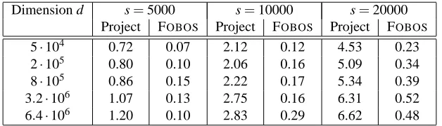
6. Efficient Implementation in High Dimensions
In many settings, especially online learning, the weight vectorwtand the gradientsgtf reside in a very
high-dimensional space, but only a relatively small number of the components ofgtf are non-zero. Such settings are prevalent, for instance, in text-based applications: in text categorization, the full dimension corresponds to the dictionary or set of tokens that is being employed while each gradient is typically computed from a single or a few documents, each of which contains words and bigrams constituting only a small subset of the full dictionary. The need to cope with gradient sparsity becomes further pronounced in mixed-norm problems, as a single component of the gradient may correspond to an entire row of W . Updating the entire matrix because a few entries ofgtf are non-zero is clearly undesirable. Thus, we would like to extend our methods to cope
efficiently with gradient sparsity. For concreteness, we focus in this section on the efficient implementation ofℓ1,ℓ2, andℓ∞regularization, recognizing that the extension to mixed-norms (as in the previous section) is
straightforward. The upshot of following proposition is that whengtf is sparse, we can use lazy evaluation of the weight vectors and defer to later rounds the update of components ofwt whose corresponding gradient
entries are zero. We detail this after the proposition, which is technical so the interested reader may skip the proof to see the simple algorithms for lazy evaluation.
Proposition 11 LetwT be the end result of solving a succession of T self-similar optimization problems for
t=1, . . . ,T ,
P
.1 : wt=argminw
1
2kw−wt−1k
2+λ
tkwkq . (28)
Letw⋆be the optimal solution of the following optimization problem:
P
.2 : w⋆=argminw
1
2kw−w0k
2+
∑
Tt=1
λt
!
kwkq .
Then for q∈ {1,2,∞}the vectorswT andw⋆are identical.
Note that the objective functions are separable for q=1. Therefore, forℓ1-regularization it suffices to
prove the proposition for any component of the vectorw. We omit the index of the component and denote by w0,w1,w2,w3, . . .one coordinate ofwalong the iterations of
P
.1 and by w⋆the result for the same component when solvingP
.2. We need to show that w⋆=w2. Expanding theℓ1-update of Eq. (19) over two iterationswe get the following,
w2=sign(w1) [|w1| −λ2]+=sign(w1)
sign(w0) [|w0| −λ1]+ −λ2
+=sign(w0) [|w0| −λ1−λ2]+ , where we used the positivity of| · |. Examining
P
.2 and using Eq. (19) again we getw⋆=sign(w0) [|w0| −λ1−λ2]+ .
Therefore, w⋆=w2as claimed.
Next we prove the proposition forℓ2, returning to using the entire vector for the proof. Using the explicit ℓ2-update from Eq. (20), we can expand the norm of the vectorw1due to the program
P
.1 as follows,kw1k =
1− λ1
kw0k
+
kw0k = [kw0k −λ1]+ .
Similarly, we get thatkw2k= [kw1k −λ2]+. Combining the norm equalities we see that the norm ofw2due
to the succession of the two updates is
kw2k = [kw0k −λ1]+−λ2+ = [kw0k −λ1−λ2]+ .
Computing directly the norm ofw⋆due to the update given by Eq. (20) yields
kw⋆k =
1−λ1+λ2
kw0k
+
kw0k = [kw0k −λ1−λ2]+ .
Thus,w⋆andw2have the same norm. Since the update itself retains the direction of the original vectorw0,
we get thatw⋆=w2as needed.
We now turn to the most complicated update and proof of the three norms, the ℓ∞ norm. We start by recapping the programs
P
.1 andP
.2 for T=2 and q=∞,P
.1 : w1 = argmin w1
2kw−w0k
2+λ 1kwk∞
(29)
w2 = argmin w
1
2kw−w1k
2+λ 2kwk∞
, (30)
P
.2 : w⋆ = argminw
1
2kw−vk
2
2+ (λ1+λ2)kwk∞
. (31)
We prove the equivalence of the two programs in two stages. First, we examine the casekw0k1>λ1+λ2,
and then consider the complement casekw0k1≤λ1+λ2. For concreteness and simplicity, we assume that
w00, since, clearly, the objective is symmetric inw0and−w0. We thus can assume that all entries of
w0are non-negative. In the proof we use the following operators:[v]+now denotes the positive component of each entry ofv, min{v,θ}denotes the component-wise minimum between the elements ofv andθ, and likewise max{v,θ}is the component-wise maximum. Starting with the casekw0k1>λ1+λ2, we examine
Eq. (29). From Lagrange duality we know that thatw1=w0−α1, whereα1is the solution of
minimize
α
1
2kα−w0k
2
2 s.t. kαk1≤λ1 .
As described by Duchi et al. (2008) and reviewed above in Sec. 5,α1= [w0−θ1]+for someθ1∈R+. The form ofα1readily translates to the following form forw1:w1=w0−α1=min(w0,θ1). Applying similar
reasoning to the second step of
P
.1 yieldsw2=w1−α2=w0−α1−α2, whereα2is the minimizer of1
2kα−w1k
2 2=
1
2kα−(w0−α1)k
2
Again, we haveα2= [w1−θ2]+= [w0−α1−θ2]+for someθ2∈R+. The successive steps then imply that
w2=min{w1,θ2}=min{min{w0,θ1},θ2} .
We next show that regardless of theℓ1-norm ofw0,θ2≤θ1. Intuitively, ifθ2>θ1, the second
minimiza-tion step of
P
.1 would perform no shrinkage ofw1to getw2. Formally, assume for the sake of contradictionthatθ2>θ1. Under this assumption, we would have thatw2=min{min{w0,θ1},θ2}=min{w0,θ1}=w1.
In turn, we obtain that0belongs to the subgradient set of Eq. (30) when evaluated atw=w1, thus,
0∈w1−w1+λ2∂kw1k∞=λ2∂kw1k∞ .
Clearly, the set∂kw1k∞can contain0only whenw1=0. Since we assumed thatλ1<kw0k1, and hence
thatα1w0andα16=w0, we have thatw1=w0−α16=0. This contradiction implies thatθ2≤θ1.
We now examine the solution vectors to the dual problems of
P
.1,α1andα2. We know thatkα1k1=λ1 so thatkw0−α1k1>λ2and henceα2is at the boundary kα2k1=λ2 (see again Duchi et al. 2008).
Furthermore, the sum of the these vectors is
α1+α2= [w0−θ1]++w0−[w0−θ1]+−θ2+. (32)
Let v denote a component ofw0greater thanθ1. For any such component the right hand side of Eq. (32)
amounts to
[v−(v−θ1)−θ2]++ [v−θ1]+= [θ1−θ2]++v−θ1=v−θ1= [v−θ1]+ ,
where we used the fact thatθ2≤θ1to eliminate the term [θ1−θ2]+. Next, let u denote a component of w0smaller than θ1. In this case, the right hand side of Eq. (32) amounts to[u−0−θ2]++0= [u−θ2]+. Recapping, the end result is that the vector sumα1+α2equals[w0−θ2]+. Moreover,α1andα2are inRn+ as we assumed thatw00, and thus
k[w0−θ2]+k1=kα1+α2k1=λ1+λ2 . (33)
We now show that
P
.2 has the same dual solution as the sequential updates above. The dual ofP
.2 isminimize
α
1
2kα−w0k
2
2 s.t. kαk1≤λ1+λ2.
Denoting byα0the solution of the above dual problem, we havew⋆=w0−α0andα0= [w0−θ]+ for someθ∈R+. Examining the norm ofα0we obtain that
kα0k1=
[w0−θ]+
1=λ1+λ2 (34)
because we assumed that kw0k1>λ1+λ2. We can view the terms
[w0−θ2]+
1 from Eq. (33) and
[w0−θ]+
1 from Eq. (34) as functions of θ2 andθ, respectively. The functions are strictly decreasing
functions ofθandθ2over the interval[0,kw0k∞]. Therefore, they are invertible for 0<λ1+λ2<kw0k1.
Since[w0−θ]+
1=
[w0−θ2]+
1, we must haveθ2=θ. Recall that the solution of Eq. (31) isw ⋆=
min{w0,θ}, and the solution of the sequential update induced by Eq. (29) and Eq. (30) is
min{min{w0,θ1},θ2} =min{w0,θ2}. The programs
P
.1 andP
.2 therefore result in the same vectormin{w0,θ2}=min{w0,θ}and their induced updates are equivalent.
We now examine the case whenkw0k1≤λ1+λ2. If the 1-norm ofw0is also smaller thanλ1,kw0k1≤λ1,
then the dual solution for the first step of
P
.1 isα1=w0, which makesw1=w0−α1=0and hencew2=0.The dual solution for the combined problem is clearlyα0=w0; again,w⋆=w0−α0=0. We are thus left
someθ1≥0, we know that each component ofα1is between zero and its corresponding component inw0,
therefore,kw0−α1k1=kw0k1− kαk1=kw0k1−λ1≤λ2. The dual of the second step of
P
.1 distills tothe minimization 12kα−(w0−α1)k2subject tokαk1≤λ2. Since we showed thatkw0−αk1≤λ2, we get
α2=w0−α1. This means thatθ2=0. Recall that the solution of
P
.1 is min{w0,θ2}, which amounts tothe zero vector whenθ2=0. We have thus showed that both optimization problems result in the zero vector.
This proves the equivalence of
P
.1 andP
.2 for q=∞.The algorithmic consequence of Proposition 11 is that it is possible to perform a lazy update on each iteration by omitting the terms ofwt (or whole rows of the matrix Wt when using mixed-norms) that are
outside the support of gtf, the gradient of the loss at iteration t. However, we do need to maintain the step-sizes used on each iteration and have them readily available on future rounds when we need to update coordinates ofwor W that were not updated in previous rounds. LetΛtdenote the sum of the step sizes times
regularization multipliersληtused from round 1 through t. Then a simple algebraic manipulation yields that
instead of solving
wt+1=argmin w
1
2kw−wtk
2
2+ληtkwkq
repeatedly whenwt is not being updated, we can simply cache the last time t0thatw(or a coordinate inw or a row from W ) was updated and, when it is needed, solve
wt+1=argmin w
1
2kw−wtk
2
2+ (Λt−Λt0)kwkq
.
The advantage of the lazy evaluation is pronounced when using mixed-norm regularization as it lets us avoid updating entire rows so long as the row index corresponds to a zero entry of the gradientgtf. We would like
to note that the lazy evaluation due to Proposition 11 includes as a special case the efficient implementation forℓ1-regularized updates first outlined by Langford et al. (2008). In sum, at the expense of keeping a time
stamp t for each entry ofwor row of W and maintaining a list of the cumulative sumsΛ1,Λ2, . . ., we can get O(s)updates ofwwhen the gradientgtf is s-sparse, that is, it has only s non-zero components.
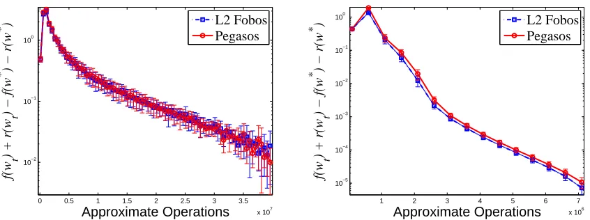
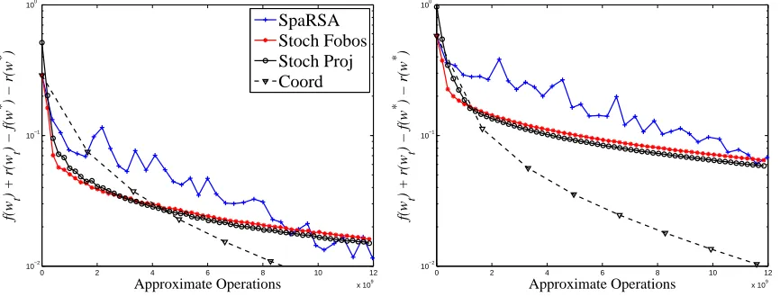
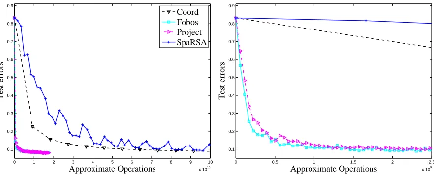
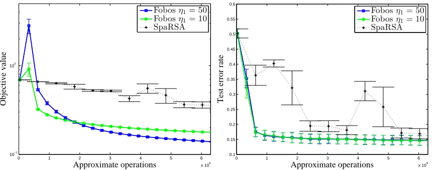
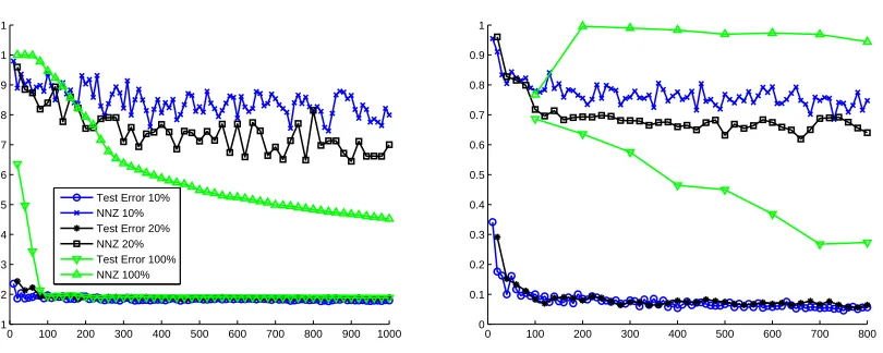
7. Experiments
In this section we describe the results of experiments we performed whose goal are to demonstrate the merits and underscore a few weaknesses of FOBOS. To that end, we also evaluate specific instantiations of FOBOS
with respect to several state-of-the-art optimizers and projected subgradient methods on different learning problems. In the experiments that focus on efficiency and speed of convergence, we evaluate the methods in terms of their number of operations, which is approximately the number of floating point operations each method performs. We believe that this metric offers a fair comparison of the different algorithms as it lifts the need to cope with specific code optimization such as cache locality or different costs per iteration of each of the methods.
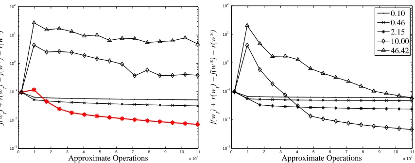
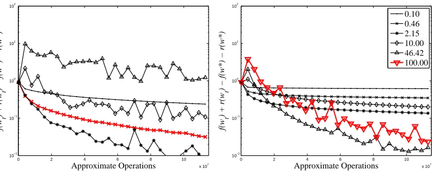
7.1 Sensitivity Experiments
We begin our experiments by performing a sensitivity analysis of FOBOS. We perform some of the analysis in later sections during our comparisons to other methods, but we discuss the bulk of it here. We focus on two tasks in our sensitivity experiments: minimizing the hinge loss (used in Support Vector Machines) with ℓ2
2regularization and minimizing theℓ1-regularized logistic loss. These set the loss function f as
f(w) =
1 n
n
∑
i=1
[1−yihxi,wi]++λ 2kwk
2
2 and f(w) =
1 n
n
∑
i=1
log
1+e−yihxi,wi+λk wk1
respectively. Note that both loss functions have subgradient sets bounded by 1n∑ni=1kyixik2. Therefore, if all