Manifold Learning: The Price of Normalization

Manifold Learning: The Price of Normalization

Yair Goldberg [email protected]

Department of Statistics The Hebrew University 91905 Jerusalem, Israel

Alon Zakai [email protected]

Interdisciplinary Center for Neural Computation The Hebrew University

91905 Jerusalem, Israel

Dan Kushnir [email protected]

Department of Computer Science and Applied Mathematics The Weizmann Institute of Science

76100 Rehovot, Israel

Ya’acov Ritov [email protected]

Department of Statistics The Hebrew University 91905 Jerusalem, Israel

Editor: Sam Roweis

Abstract

We analyze the performance of a class of manifold-learning algorithms that find their output by minimizing a quadratic form under some normalization constraints. This class consists of Locally Linear Embedding (LLE), Laplacian Eigenmap, Local Tangent Space Alignment (LTSA), Hessian Eigenmaps (HLLE), and Diffusion maps. We present and prove conditions on the manifold that are necessary for the success of the algorithms. Both the finite sample case and the limit case are analyzed. We show that there are simple manifolds in which the necessary conditions are violated, and hence the algorithms cannot recover the underlying manifolds. Finally, we present numerical results that demonstrate our claims.

Keywords: dimensionality reduction, manifold learning, Laplacian eigenmap, diffusion maps, locally linear embedding, local tangent space alignment, Hessian eigenmap

1. Introduction

Coifman and Lafon, 2006).

These manifold-learning algorithms compute an embedding for some given input. It is assumed that this input lies on a low-dimensional manifold, embedded in some high-dimensional space. Here a manifold is defined as a topological space that is locally equivalent to a Euclidean space. It is further assumed that the manifold is the image of a low-dimensional domain. In particular, the input points are the image of a sample taken from the domain. The goal of the manifold-learning algorithms is to recover the original domain structure, up to some scaling and rotation. The non-linearity of these algorithms allows them to reveal the domain structure even when the manifold is not linearly embedded.

The central question that arises when considering the output of a manifold-learning algorithm is, whether the algorithm reveals the underlying low-dimensional structure of the manifold. The answer to this question is not simple. First, one should define what “revealing the underlying lower-dimensional description of the manifold” actually means. Ideally, one could measure the degree of similarity between the output and the original sample. However, the original low-dimensional data representation is usually unknown. Nevertheless, if the low-dimensional structure of the data is known in advance, one would expect it to be approximated by the dimension-reducing algorithm, at least up to some rotation, translation, and global scaling factor. Furthermore, it would be reasonable to expect the algorithm to succeed in recovering the original sample’s structure asymptotically, namely, when the number of input points tends to infinity. Finally, one would hope that the algorithm would be robust in the presence of noise.

Previous papers have addressed the central question posed earlier. Zhang and Zha (2004) pre-sented some bounds on the local-neighborhoods’ error-estimation for LTSA. However, their analysis says nothing about the global embedding. Huo and Smith (2006) proved that, asymptotically, LTSA recovers the original sample up to an affine transformation. They assume in their analysis that the level of noise tends to zero when the number of input points tends to infinity. Bernstein et al. (2000.) proved that, asymptotically, the embedding given by the Isomap algorithm (Tenenbaum et al., 2000) recovers the geodesic distances between points on the manifold.

In this paper we develop theoretical results regarding the performance of a class of manifold-learning algorithms, which includes the following five algorithms: Locally Linear Embedding (LLE), Laplacian Eigenmap (LEM), Local Tangent Space Alignment (LTSA), Hessian Eigenmaps (HLLE), and Diffusion maps (DFM).

We refer to this class of algorithms as the normalized-output algorithms. The normalized-output algorithms share a common scheme for recovering the domain structure of the input data set. This scheme is constructed in three steps. In the first step, the local neighborhood of each point is found. In the second step, a description of these neighborhoods is computed. In the third step, a low-dimensional output is computed by solving some convex optimization problem under some normalization constraints. A detailed description of the algorithms is given in Section 2.

as an explanatory introduction to the more general analysis that appears in Section 5. Some of the ideas that form the basis of the analysis in Section 4 were discussed independently by both Gerber et al. (2007) and ourselves (Goldberg et al., 2007). Section 5 finds necessary conditions for the suc-cessful performance of all the normalized-output algorithms on general two-dimensional manifolds. It should be noted that the necessary conditions are hard to verify in practice. However, they serve as an analytic tool to prove that there are general classes of manifolds on which the normalized-output algorithms fail. Moreover, the numerical examples in this section show that the class of manifolds on which the normalized-output algorithms fail is wide and includes non-isometrically manifolds and real-world data. In Section 6 we discuss the performance of the algorithms in the asymptotic case. Concluding remarks appear in Section 7. The detailed proofs appear in the Appendix.

Our paper has two main results. First, we give well-defined necessary conditions for the suc-cessful performance of the normalized-output algorithms. Second, we show that there exist simple manifolds that do not fulfill the necessary conditions for the success of the algorithms. For these manifolds, the normalized-output algorithms fail to generate output that recovers the structure of the original sample. We show that these results hold asymptotically for LEM and DFM. Moreover, when noise, even of small variance, is introduced, LLE, LTSA, and HLLE will fail asymptotically on some manifolds. Throughout the paper, we present numerical results that demonstrate our claims.

2. Description of Output-normalized Algorithms

In this section we describe in short the normalized-output algorithms. The presentation of these algorithms is not in the form presented by the respective authors. The form used in this paper emphasizes the similarities between the algorithms and is better-suited for further derivations. In Appendix A.1 we show the equivalence of our representation of the algorithms and the representa-tions that appear in the original papers.

Let X = [x1, . . . ,xN]0,xi∈RD be the input data where

D

and N is the size of the sample. The normalized-output algorithms attempt to recover the underlying structure of the input data X in three steps.

In the first step, the normalized-output algorithms assign neighbors to each input point xibased

on the Euclidean distances in the high-dimensional space.1 This can be done, for example, by

choos-ing all the input points in an r-ball around xior alternatively by choosing xi’s K-nearest-neighbors.

The neighborhood of xi is given by the matrix Xi= [xi,xi,1, . . . ,xi,K]0 where xi,j: j=1, . . . ,K are

the neighbors of xi. Note that K=K(i) can be a function of i, the index of the neighborhood, yet

we omit this index to simplify the notation. For each neighborhood, we define the radius of the neighborhood as

r(i) = max

j,k_∈{0,...,K_}

xi,j−xi,k

where we define xi,0=xi. Finally, we assume throughout this paper that the neighborhood graph is

connected.

In the second step, the normalized-output algorithms compute a description of the local neigh-borhoods that were found in the previous step. The description of the i-th neighborhood is given by

some weight matrix Wi. The matrices Wi for the different algorithms are presented.

Wi=       

w1/2_{i,1 −}w1/2_i,1 0 _··· 0 w1/2_i,2 0 ₋w1/2_i,2 . .. ...

..

. ... . .. . .. 0

w1/2_i,K 0 _··· 0 ₋w1/2_i,K

       .

For LEM wi,j=1 is a natural choice, yet it is also possible to define the weights as ˜wi,j=

e−kxi−xi,jk

2

/ε_{, whereεis the width parameter of the kernel. For the case of DFM,}

wi,j=

k_ε(xi,xi,j)

qε(xi)αqε(xi,j)α

, (1)

where k_ε is some rotation-invariant kernel, q_ε(xi) =∑jkε(xi,xi,j) andεis again a width

pa-rameter. We will useα=1 in the normalization of the diffusion kernel, yet other values of

αcan be considered (see details in Coifman and Lafon, 2006). For both LEM and DFM, we

define the matrix D to be a diagonal matrix where dii=∑jwi,j.

• LLE: Wiis a 1×(K+1)matrix,

Wi= 1 −wi,1 ··· −wi,K

.

The weights wi,j are chosen so that xi can be best linearly reconstructed from its neighbors.

The weights minimize the reconstruction error function

∆i_(w

i,1, . . . ,wi,K) =kxi−

∑

wi,jxi,jk2

under the constraint∑jwi,j=1. In the case where there is more than one solution that

mini-mizes∆i, regularization is applied to force a unique solution (for details, see Saul and Roweis,

2003).

• LTSA: Wiis a(K+1)×(K+1)matrix,

Wi= (I−PiPi0)H.

Let UiLiVi0be the SVD of Xi−1 ¯x0iwhere ¯xiis the sample mean of Xiand 1 is a vector of ones

(for details about SVD, see, for example, Golub and Loan, 1983). Let Pi = [u(1), . . . ,u(d)]

be the matrix that holds the first d columns of Ui where d is the output dimension. The

matrix H=I_−K1110 is the centering matrix. See also Huo and Smith (2006) regarding this

representation of the algorithm.

• HLLE: Wi is a d(d+1)/2×(K+1)matrix,

Wi= (0,Hi)

where 0 is a vector of zeros and Hi is thed(d₂+1)_×K Hessian estimator.

The estimator can be calculated as follows. Let UiLiVi0be the SVD of Xi−1 ¯x0i. Let

Mi= [1,U(

1) i , . . . ,U

(d)

i ,diag(U

(1)

i U

(1)

i 0),diag(U (1)

i U

(2)

i 0), . . . ,diag(U (d)

i U

where the operator diag returns a column vector formed from the diagonal elements of the

matrix. Let Mei be the result of the Gram-Schmidt orthonormalization on Mi. Then Hi is

defined as the transpose of the last d(d+1)/2 columns ofMei.

The third step of the normalized-output algorithms is to find a set of points Y = [y1, . . . ,yN]0,yi∈

Rd _{where d≤}

D

under some normalization constraints, as follows. Let Y be any N×d matrix. We define the i-th

neighborhood matrix Yi= [yi,yi,1, . . . ,yi,K]0 using the same pairs of indices i,j as in Xi. The cost

function for all of the normalized-output algorithms is given by

Φ(Y) =

N

∑

i=1

φ(Yi) = N

∑

i=1

kWiYik2F , (2)

under the normalization constraints

Y0DY =I

Y0D1=0 for LEM and DFM,

Cov(Y) =I

Y01=0 for LLE,LTSA and HLLE, (3)

where_{k kF} stands for the Frobenius norm, and Wi is algorithm-dependent.

Define the output matrix Y to be the matrix that achieves the minimum ofΦunder the

normaliza-tion constraints of Eq. 3 (Y is defined up to rotanormaliza-tion). Then we have the following: the embeddings of LEM and LLE are given by the according output matrices Y ; the embeddings of LTSA and HLLE

are given by the according output matrices √1

NY ; and the embedding of DFM is given by a linear

transformation of Y as discussed in Appendix A.1. The discussion of the algorithms’ output in this paper holds for any affine transformation of the output (see Section 3). Thus, without loss of gen-erality, we prefer to discuss the output matrix Y directly, rather than the different embeddings. This allows a unified framework for all five normalized-output algorithms.

3. Embedding Quality

In this section we discuss possible definitions of “successful performance” of manifold-learning algorithms. To open our discussion, we present a numerical example. We chose to work with LTSA rather arbitrarily. Similar results can be obtained using the other algorithms.

The example we consider is a uniform sample from a two-dimensional strip, shown in Fig. 1A.

Note that in this example,

D

A B C D

E F G

Figure 1: The output of LTSA (B) for the (two-dimensional) input shown in (A), where the input

is a uniform sample from the strip[0,1]_×[0,6]. Ideally one would expect the two to be

identical. The normalization constraint shortens the horizontal distances and lengthens the vertical distances, leading to the distortion of geodesic distances. (E) and (F) focus on the points shown in black in (A) and (B), respectively. The (blue) triangles pointing downwards in (E) and (F) are the 8-nearest-neighborhood of the point denoted by the full black circle. The (red) triangles pointing upwards in (F) indicate the neighborhood computed for the corresponding point (full black circle) in the output space. Note that less than half of the original neighbors of the point remain neighbors in the output space. The input (A) with the addition of Gaussian noise normal to the manifold and of variance

10−4is shown in (C). The output of LTSA for the noisy input is shown in (D). (G) shows

a closeup of the neighborhood of the point indicated by the black circle in (D).

local neighborhood. Mappings that preserve local structures up to a scale are called conformal mappings (see for example de Silva and Tenenbaum, 2003; Sha and Saul, 2005). In addition to the distortion of angles and distances, the K-nearest-neighbors of a given point on the manifold do not necessarily correspond to the K-nearest-neighbors of the respective output point, as shown in Figs. 1E and 1F. Accordingly, we conclude that the original structure of the local neighborhoods is not necessarily preserved by the normalized-output algorithms.

normalized-output algorithm succeeds (or fails) based on the existence (or lack thereof) of resem-blance between the output and the original sample, up to an affine transformation.

Fig. 1D presents the output of LTSA on a noisy version of the input, shown in Fig. 1C. In

this case, the algorithm prefers an output that is roughly a one-dimensional curve embedded inR2_.

While this result may seem incidental, the results of all the other normalized-output algorithms for this example are essentially the same.

Using the affine transformation criterion, we can state that LTSA succeeds in recovering the underlying structure of the strip shown in Fig. 1A. However, in the case of the noisy strip shown in Fig. 1C, LTSA fails to recover the structure of the input. We note that all the other normalized-output algorithms perform similarly.

For practical purposes, we will now generalize the definition of failure of the normalized-output algorithms. This definition is more useful when it is necessary to decide whether an algorithm has failed, without actually computing the output. This is useful, for example, when considering the outputs of an algorithm for a class of manifolds.

We now present the generalized definition of failure of the algorithms. Let X =XN×d be the

original sample. Assume that the input is given by ψ(X)_⊂RD_{, where} ψ_:Rd _→RD _{is some}

smooth function, and

D

of the original sample X , such that the normalization constraints of Eq. 3 hold. Note that Y is algorithm-dependent, and that for each algorithm, Y is unique up to rotation and translation. When the algorithm succeeds it is expected that the output will be similar to a normalized version of X ,

namely to Y . Let Z=ZN×d be any matrix that satisfies the same normalization constraints. We say

that the algorithm has failed if Φ(Y)>Φ(Z), and Z is substantially different from Y , and hence

also from X . In other words, we say that the algorithm has failed when a substantially different embedding Z has a lower cost than the most appropriate embedding Y . A precise definition of “substantially different” is not necessary for the purposes of this paper. It is enough to consider Z substantially different from Y when Z is of lower dimension than Y , as in Fig. 1D.

We emphasize that the matrix Z is not necessarily similar to the output of the algorithm in question. It is a mathematical construction that shows when the output of the algorithm is not likely to be similar to Y , the normalized version of the true manifold structure. The following lemma

shows that ifΦ(Y)>Φ(Z), the inequality is also true for a small perturbation of Y . Hence, it is not

likely that an output that resembles Y will occur whenΦ(Y)>Φ(Z)and Z is substantially different

from Y .

Lemma 3.1 Let Y be an N_×d matrix. LetYe=Y+εE be a perturbation of Y , where E is an N_×d matrix such that_kE_kF =1 and whereε>0. Let S be the maximum number of neighborhoods to which a single input point belongs. Then for LLE with positive weights wi,j, LEM, DFM, LTSA, and

HLLE, we have

Φ(Ye)>(1₋ε)Φ(Y)₋εCaS,

where Cais a constant that depends on the algorithm.

The use of positive weights in LLE is discussed in Saul and Roweis (2003, Section 5); a similar

result for LLE with general weights can be obtained if one allows a bound on the values of wi,j. The

A B C

A B C

A B C

A B C

A B C

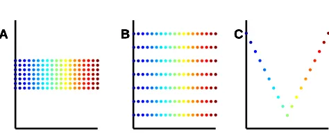
Figure 2: (A) The input grid. (B) Embedding Y , the normalized grid. (C) Embedding Z, a curve

that satisfies Cov(Z) =I.

4. Analysis of the Two-Dimensional Grid

In this section we analyze the performance of LEM on the two-dimensional grid. In particular, we argue that LEM cannot recover the structure of a two-dimensional grid in the case where the

aspect ratio of the grid is greater than 2. Instead, LEM prefers a one-dimensional curve in R2_.

Implications also follow for DFM, as explained in Section 4.3, followed by a discussion of the other normalized-output algorithms. Finally, we present empirical results that demonstrate our claims.

In Section 5 we prove a more general statement regarding any two-dimensional manifold. Nec-essary conditions for successful performance of the normalized-output algorithms on such mani-folds are presented. However, the analysis in this section is important in itself for two reasons. First, the conditions for the success of LEM on the two-dimensional grid are more limiting. Sec-ond, the analysis is simpler and points out the reasons for the failure of all the normalized-output algorithms when the necessary conditions do not hold.

4.1 Possible Embeddings of a Two-Dimensional Grid

We consider the input data set X to be the two-dimensional grid[₋m, . . . ,m]_×[₋q, . . . ,q], where m_≥q. We denote xi j = (i,j). For convenience, we regard X = (X(1),X(2)) as an N×2 matrix,

where N= (2m+1)(2q+1)is the number of points in the grid. Note that in this specific case, the

original sample and the input are the same.

In the following we present two different embeddings, Y and Z. Embedding Y is the grid itself,

normalized so that Cov(Y) =I. Embedding Z collapses each column to a point and positions the

resulting points in the two-dimensional plane in a way that satisfies the constraint Cov(Z) =I (see

Fig. 2 for both). The embedding Z is a curve in R2 _{and clearly does not preserve the original}

structure of the grid.

We first define the embeddings more formally. We start by definingYb=X(X0DX)−1/2. Note that

this is the only linear transformation of X (up to rotation) that satisfies the conditionsYb0D1=0 and

b

Y0DYb=I, which are the normalization constraints for LEM (see Eq. 3). However, the embedding

b

Y depends on the matrix D, which in turn depends on the choice of neighborhoods. Recall that the

matrix D is a diagonal matrix, where diiequals the number of neighbors of the i-th point. Choose r

to be the radius of the neighborhoods. Then, for all inner points xi j, the number of neighbors K(i,j)

points. Note that the definition of boundary points depends on the choice of r. For inner points of

the grid we have dii≡K. Thus, when KN we have X0DX≈KX0X .

We define Y =X Cov(X)−1/2. Note that Y01=0, Cov(Y) =I and for K N, Y _≈√KNY .b

In this section we analyze the embedding Y instead ofY , thereby avoiding the dependence on theb

matrix D and hence simplifying the notation. This simplification does not significantly change the problem and does not affect the results we present. Similar results are obtained in the next section for general two-dimensional manifolds, using the exact normalization constraints (see Section 5.2). Note that Y can be described as the set of points [₋m/σ, . . . ,m/σ]_×[₋q/τ, . . . ,q/τ], where yi j = (i/σ,j/τ). The constantsσ2 =Var(X(1)) andτ2=Var(X(2)) ensure that the normalization

constraint Cov(Y) =I holds. Straightforward computation (see Appendix A.3) shows that

σ2₌(m+1)m

3 ;τ

2₌(q+1)q

3 . (4)

The definition of the embedding Z is as follows:

zi j=       

i

σ,−ρ2i−¯z(2)

i_≤0

i

σ,2iρ−¯z(2)

i_≥0 ,

where ¯z(2)= (2q_N+_ρ1)2∑m_i=1(2i)ensures that Z01=0, andσ(the sameσas before; see below) and ρ

are chosen so that sample variance of Z(1) and Z(2)is equal to one. The symmetry of Z(1) about

the origin implies that Cov(Z(1)_,Z(2)_{) =0, hence the normalization constraint Cov(Z) =I holds. σ}

is as defined in Eq. 4, since Z(1)=Y(1)(with both defined similarly to X(1)). Finally, note that the definition of zi jdoes not depend on j.

4.2 Main Result for LEM on the Two-Dimensional Grid

We estimate Φ(Y) by Nφ(Yi j) (see Eq. 2), where yi j is an inner point of the grid and Yi j is the

neighborhood of yi j; likewise, we estimateΦ(Z) by Nφ(Zi j)for an inner point zi j. For all inner

points, the value of φ(Yi j)is equal to some value φ. For boundary points,φ(Yi j)is bounded byφ

multiplied by some constant that depends only on the number of neighbors. Hence, for large m and q, the difference betweenΦ(Y)and Nφ(Yi j)is negligible.

The main result of this section states:

Theorem 4.1 Let yi j be an inner point and let the ratio m_q be greater than 2. Then

φ(Yi j)>φ(Zi j)

for neighborhood-radius r that satisfies 1_≤r_≤3, or similarly, for K-nearest neighborhoods where K=4,8,12.

This indicates that for aspect ratios m_q that are greater than 2 and above, mapping Z, which is

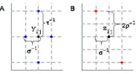
Figure 3: (A) The normalized grid at an inner point yi j. The 4-nearest-neighbors of yi j are marked

in blue. Note that the neighbors from the left and from the right are at a distance of 1/σ, while the neighbors from above and below are at a distance of 1/τ. The value of

φ(Yi j)is equal to the sum of squared distances of yi j to its neighbors. Hence, we obtain

thatφ(Yi j) =2/σ2+2/τ2when K=4 andφ(Yi j) =2/σ2+2/τ2+4(1/σ2+1/τ2)when

K=8. (B) The curve embedding at an inner point zi j. The neighbors of zi j from the left

and from the right are marked in red. The neighbors from above and below are embedded to the same point as zi j. Note that the squared distance between zi j and z(i±1)j equals

1/σ2_+4/ρ2_{. Hence,φ(Z}

i j) =2(1/σ2+4/ρ2)when K=4, andφ(Zi j) =6(1/σ2+4/ρ2)

when K=8.

The proof of the theorem is as follows. It can be shown analytically (see Fig. 3) that

φ(Yi j) =F(K)

1 σ2+

1 τ2

, (5)

where

F(4) =2 ; F(8) =6 ; F(12) =14.

For higher K, F(K)can be approximated for any r-ball neighborhood of yi j (see Appendix A.4).

It can be shown (see Fig. 3) that

φ(Zi j) =F(K)e

1 σ2+

4 ρ2

, (6)

where Fe(K) =F(K) for K =4,8,12. For higher K, it can be shown (see Appendix A.4) that

e

F(K)_≈F(K)for any r-ball neighborhood.

A careful computation (see Appendix A.5) shows that

ρ>σ, (7)

and therefore

φ(Zi j)<

5F(K)

Assume that m_q >2. Since both m and q are integers, we have that m+1≥2(q+1). Hence, using Eq. 4 we have

σ2₌m(m+1)

3 >

4q(q+1)

3 =4τ

2_. Combining this result with Eqs. 5 and 8 we have

m

q >2⇒φ(Yi j)>φ(Zi j)

which proves Theorem 4.1.

4.3 Implications to Other Algorithms

We start with implications regarding DFM. There are two main differences between LEM and DFM.

The first difference is the choice of the kernel. LEM chooses wi,j=1, which can be referred to as

the “window” kernel (a Gaussian weight function was also considered by Belkin and Niyogi, 2003). DFM allows a more general rotation-invariant kernel, which includes the “window” kernel of LEM.

The second difference is that DFM renormalizes the weights k_ε(xi,xi,j)(see Eq. 1). However, for

all the inner points of the grid with neighbors that are also inner points, the renormalization factor (qε(xi)−1qε(xi,j)−1)is a constant. Therefore, if DFM chooses the “window” kernel, it is expected

to fail, like LEM. In other words, when DFM using the “window” kernel is applied to a grid with aspect ratio slightly greater than 2 or above, DFM will prefer the embedding Z over the embedding Y (see Fig 2). For a more general choice of kernel, the discussion in Appendix A.4 indicates that

a similar failure should occur. This is because the relation between the estimations of Φ(Y) and

Φ(Z)presented in Eqs. 5 and 6 holds for any rotation-invariant kernel (see Appendix A.4). This

observation is also evident in numerical examples, as shown in Figs. 4 and 5.

In the cases of LLE with no regularization, LTSA, and HLLE, it can be shown thatΦ(Y)_≡0.

Indeed, for LTSA and HLLE, the weight matrix Wiprojects on a space that is perpendicular to the

SVD of the neighborhood Xi, thus kWiXik2_F =0. Since Yi=XiCov(X)−1/2, we havekWiYik2_F =0,

and, therefore,Φ(Y)_≡0. For the case of LLE with no regularization, when K_≥3, each point can be

reconstructed perfectly from its neighbors, and the result follows. Hence, a linear transformation of

the original data should be the preferred output. However, the fact thatΦ(Y)_≡0 relies heavily on the

assumption that both the input X and the output Y are of the same dimension (see Theorem 5.1 for manifolds embedded in higher dimensions), which is typically not the case in dimension-reducing applications.

4.4 Numerical Results

For the following numerical results, we used the Matlab implementation written by the respective algorithms’ authors as provided by Wittman (retrieved Jan. 2007) (a minor correction was applied to the code of HLLE).

We ran the LEM algorithm on data sets with aspect ratios above and below 2. We present results for both a grid and a uniformly sampled strip. The neighborhoods were chosen using K-nearest

neighbors with K =4,8,16, and 64. We present the results for K=8; the results for K=4,16,

A

B

C

D

A

B

C

D

A

B

C

D

A

B

C

D

A

B

C

D

Figure 4: The output of LEM on a grid of dimensions 81_×41 is presented in (A). The result of

LEM for the grid of dimensions 81_×39 is presented in (B). The number of neighbors in

both computations is 8. The output for DFM on the same data sets usingσ=2 appears

in (C) and (D), respectively.

We ran the DFM algorithm on the same data sets. We used the normalization constant α=1

and the kernel widthσ=2; the results forσ=1,4, and 8 are similar. The results for the grid and

the random sample are presented in Figures 4 and 5, respectively.

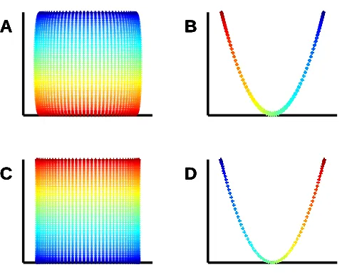
Both examples clearly demonstrate that for aspect ratios sufficiently greater than 2, both LEM and DFM prefer a solution that collapses the input data to a nearly one-dimensional output,

normal-ized inR2_{. This is exactly as expected, based on our theoretical arguments.}

Finally, we ran LLE, HLLE, and LTSA on the same data sets. In the case of the grid, both

LLE and LTSA (roughly) recovered the grid shape for K=4,8,16, and 64, while HLLE failed to

produce any output due to large memory requirements. In the case of the random sample, both LLE

and HLLE succeeded for K=16,64 but failed for K=4,8. LTSA succeeded for K=8,16, and 64

but failed for K=4. The reasons for the failure for lower values of K are not clear, but may be due

to roundoff errors. In the case of LLE, the failure may also be related to the use of regularization in LLE’s second step.

5. Analysis for General Two-Dimensional Manifolds

0 20 40 60 80 0

20 41

0 20 40 60 80 0

20 39

A B C

D E F

Figure 5: (A) and (D) show the same 3000 points, uniformly-sampled from the unit square, scaled to the areas[0,81]_×[0,41]and[0,81]_×[0,39], respectively. (B) and (E) show the outputs of LEM for inputs (A) and (D), respectively. The number of neighbors in both

computa-tions is 8. (C) and (F) show the output for DFM on the same data sets usingσ=2. Note

the sharp change in output structure for extremely similar inputs.

5.1 Two Different Embeddings for a Two-Dimensional Manifold

We start with some definitions. Let X= [x1, . . . ,xN]0,xi∈R2be the original sample. Without loss

of generality, we assume that

¯

x=0; Cov(X)_≡Σ=

_σ2

0

0 τ2

.

As in Section 4, we assume thatσ>τ. Assume that the input for the normalized-output algorithms is

given byψ(X)_⊂RD _whereψ_:R2_→RD _{is a smooth function and}

D

input. When the mappingψis an isometry, we expectΦ(X)to be small. We now take a close look

atΦ(X).

Φ(X) =

N

∑

i=1

kWiXik2F= N

∑

i=1

WiXi(1)

2+

N

∑

i=1

WiXi(2)

2,

where X_i(j) is the j-th column of the neighborhood Xi. Define e(ij)= WiXi(j)

2, and note that e(_ij)

depends on the different algorithms through the definition of the matrices Wi. The quantity e(

j)

i is the

portion of error obtained by using the j-th column of the i-th neighborhood when using the original sample as output. Denote ¯e(j)= 1

N∑ie (j)

Y =XΣ−1/2 (9) be the first embedding. Note that Y is just the original sample up to a linear transformation that

ensures that the normalization constraints Cov(Y) =I and Y01=0 hold. Moreover, Y is the only

transformation of X that satisfies these conditions, which are the normalization constraints for LLE, HLLE, and LTSA. In Section 5.2 we discuss the modified embeddings for LEM and DFM.

The second embedding, Z, is given by

zi=           

x(i1)

σ ,−x

(1)

i

ρ −¯z(2)

x(_i1)<0

x(_i1)

σ ,κx

(1)

i

ρ −¯z(2)

x(_i1)_≥0

. (10)

Here

κ=

∑

i:x(_i1)<0

x(_i1)21/2

∑

i:x_i(1)≥0

x(_i1)2−1/2 (11)

ensures that Cov(Z(1)_,Z(2)_{) =0, and ¯z}(2)₌ 1

N(∑x(_i1)≥0

κx(i1)

ρ +∑x(_i1)<0

−x(i1)

ρ )andρare chosen so that

the sample mean and variance of Z(2) are equal to zero and one, respectively. We assume without

loss of generality thatκ_≥1.

Note that Z depends only on the first column of X . Moreover, each point zi is just a linear

transformation of x(_i1). In the case of neighborhoods Zi, the situation can be different. If the first

column of Xiis either non-negative or non-positive, then Ziis indeed a linear transformation of Xi(1).

However, if X_i(1)is located on both sides of zero, Ziis not a linear transformation of Xi(1). Denote by

N0the set of indices i of neighborhoods Zithat are not linear transformations of Xi(1). The number

|N0_|depends on the number of nearest neighbors K. Recall that for each neighborhood, we defined

the radius r(i) =maxj,k∈{0,...,K}

xi,j−xi,k

. Define rmax=maxi_∈N0r(i)to be the maximum radius

of neighborhoods i, such that i_∈N0.

5.2 The Embeddings for LEM and DFM

So far we have claimed that given the original sample X , we expect the output to resemble Y (see Eq. 9). However, Y does not satisfy the normalization constraints of Eq. 3 for the cases of LEM

and DFM. Define ˆY to be the only affine transformation of X (up to rotation) that satisfies the

normalization constraint of LEM and DFM. When the original sample is given by X , we expect

the output of LEM and DFM to resemble ˆY . We note that unlike the matrix Y that was defined in

terms of the matrix X only, ˆY depends also on the choice of neighborhoods through the matrix D

that appears in the normalization constraints.

We define ˆY more formally. DenoteXe=X₋₁01_D1110DX . Note thatX is just a translation of Xe that ensures thatXe0D1=0. The matrixXe0DX is positive definite and therefore can be presented bye

ΓbΣΓ0 _{whereΓis a 2×2 orthogonal matrix and}

b

Σ=

ˆ σ2 ₀

0 ˆτ2

where ˆσ≥τ. Defineˆ Xb=XeΓ; thenYb=XbΣb−1/2is the only affine transformation of X that satisfies

the normalization constraints of LEM and DFM; namely, we haveYb0DYb=I andYb0D1=0.

We defineZ similarly to Eq. 10,b

ˆzi=            ˆ

x(_i1)

ˆ

σ ,−xˆ

(1)

i

ˆ

ρ −ˆ¯z(2)

ˆ x(_i1)<0

ˆ

x(i1)

ˆ

σ ,κˆxˆ

(1)

i

ˆ

ρ −ˆ¯z(2)

ˆ x(_i1)≥0

,

where ˆκis defined by Eq. 11 with respect toX , ˆ¯zb (2)= 1

N(∑x(i1)≥0

diiκˆx(

1)

i

ρ +∑x(i1)<0

−diix(

1)

i

ρ )and ˆρ2=

κ2_∑ ˆ

xi(1)≥0

dii

ˆ

x(_i1)2+∑ ˆ

x(i1)≤0

dii

ˆ x(_i1)2.

A similar analysis to that of Y and Z can be performed for Y andb Z. The same necessaryb

conditions for success are obtained, withσ,τ, andρreplaced by ˆσ, ˆτ, and ˆρ, respectively. In the

case where the distribution of the original points is uniform, the ratio σ_τˆ_ˆ is close to the ratio σ_τ and thus the necessary conditions for the success of LEM and DFM are similar to the conditions in Corollary 5.2.

5.3 Characterization of the Embeddings

The main result of this section provides necessary conditions for the success of the

normalized-output algorithms. Following Section 3, we say that the algorithms fail ifΦ(Y)>Φ(Z), where Y

and Z are defined in Eqs. 9 and 10, respectively. Thus, a necessary condition for the success of the

normalized-output algorithms is thatΦ(Y)_≤Φ(Z).

Theorem 5.1 Let X be a sample from a two-dimensional domain and letψ(X)be its embedding in high-dimensional space. Let Y and Z be defined as above. Then

κ2 ρ2

¯

e(1)+|N0| N car

2 max

<e¯

(2)

τ2 =⇒ Φ(Y)>Φ(Z), (12) where cais a constant that depends on the specific algorithm. For the algorithms LEM and DFM a

more restrictive condition can be defined:

κ2 ρ2e¯

(1)_<e¯(2)

τ2 =⇒ Φ(Y)>Φ(Z). For the proof, see Appendix A.6.

Note that the bound in Eq. 12 depends on the radii of the neighborhoods, and when the maxi-mum radius is large, the bound is less effective. However, there is a tradeoff between enlarging the

radius and improving the description of the neighborhoods, that is, reducing ¯e(2). In other words,

when the neighborhoods are large, one can expect a large average error in the description of the neighborhoods, since the Euclidian approximation of the neighborhoods is less accurate for neigh-borhoods of large radius.

Adding some assumptions, we can obtain a simpler criterion. First note that, in general, ¯e(1)

from a symmetric unimodal distribution it can be assumed thatκ_≈1 andρ2>σ₈. Then we have the following corollary:

Corollary 5.2 Let X,Y,Z be as in Theorem 5.1. Let c=σ/τbe the ratio between the variance of the first and second columns of X . Assume that ¯e(1)<√2 ¯e(2),κ<√4

2, andρ2>σ₈2. Then

4

1+|N0| N

carmax2 √

2 ¯e(2)

<c_⇒Φ(Y)>Φ(Z).

For LEM and DFM, we can write

4<c_⇒Φ(Y)>Φ(Z).

We emphasize that both Theorem 5.1 and Corollary 5.2 do not state that Z is the output of the normalized-output algorithms. However, when the difference between the right side and the left side of the inequalities is large, one cannot expect the output to resemble the original sample (see Lemma 3.1). In these cases we say that the algorithms fail to recover the structure of the original domain.

5.4 Generalization of the Results to Manifolds of Higher Dimensions

The discussion above introduced necessary conditions for the normalized-output algorithms’

suc-cess on two-dimensional manifolds embedded inRD_{. Necessary conditions for success on general}

d-dimensional manifolds, d_≥3, can also be obtained. We present here a simple criterion to demon-strate the fact that there are d-dimensional manifolds that the normalized-output algorithms cannot recover.

Let X = [X(1)_{, . . . ,X}(d)_{]be a N×d sample from a d-dimensional domain. Assume that the input}

for the normalized-output algorithms is given byψ(X)_⊂RD _whereψ_:Rd_→RD _{is a smooth}

func-tion and

D

that Cov(X)is a diagonal matrix. Let Y =X Cov(X)−1/2. We define the matrix Z= [Z(1)_{, . . . ,Z}(d)_]

as follows. The first column of Z, Z(1), equals the first column of Y , namely, Z(1)=Y(1). We define

the second column Z(2)similarly to the definition in Eq. 10:

Z_i(2)=

      

−x(i1)

ρ −¯z(2) x(i1)<0

κx(i1)

ρ −¯z(2) x(i1)≥0

, (13)

whereκis defined as in Eq. 11, and ¯z(2)andρare chosen so that the sample mean and variance of

Z(2)are equal to zero and one, respectively. We define the next d₋2 columns of Z by

Z(j)=Y

(j)_{−σ2 jZ}(2) q

1₋σ2_{2 j}

; j=3, . . . ,d,

We boundΦ(Z)from above:

Φ(Z) = Φ(Y(1)_{) +Φ(Z}(2)_{) +}

∑

1 1₋σ2_{2 j}

! d

∑

j=3

Wi

Y_i(j)₋σ2 jZ_i(2)2

≤ Φ(Y(1)_{) +Φ(Z}(2)_{) +} 1

1₋σ2 max

N

∑

i=1

d

∑

j=3

WiYi(j)

2+ σ

2 max 1₋σ2

max

N

∑

i=1

d

∑

j=3

WiZi(2)

2

= Φ(Y(1)) +1+ (d−3)σ 2 max 1₋σ2

max

Φ(Z(2)_{) +} 1

1₋σ2 max

d

∑

j=3

Φ(Y(j)_).

Since we may writeΦ(Y) =∑d

j=1Φ(Y(j)), we have

1+ (d₋3)σ2

max 1₋σ2

max

Φ(Z(2)_)<Φ(Y(2)_{) +} σ2max 1₋σ2

max

d

∑

j=3

Φ(Y(j)_{)⇒Φ(Z)<Φ(Y).}

When the sample is taken from a symmetric distribution with respect to the axes, one can expect σmaxto be small. To see this, note that by symmetry and Eq. 13, Z_i(2)_{≈ |}Y_i(1)_|, and by assumption Cov(Y(1)_,Y(j)_{) =0 for j=3, . . . ,d. Hence, by the symmetry of Y}(j)_{,σ2 j is expected to be small.}

In the specific case of the d-dimensional grid, σmax=0. Indeed, Y(j) is symmetric around zero,

and all values of Z(2)appear for a given value of Y(j). Hence, both LEM and DFM are expected to

fail whenever the ratio between the length of the grid in the first and second coordinates is slightly greater than 2 or more, regardless of the length of grid in the other coordinates, similar to the result presented in Theorem 4.1. Corresponding results for the other normalized-output algorithms can also be obtained, similar to the derivation of Corollary 5.2.

5.5 Numerical Results

We ran all five normalized-output algorithms, along with Isomap, on three data sets. We used the Matlab implementations written by the algorithms’ authors as provided by Wittman (retrieved Jan. 2007).

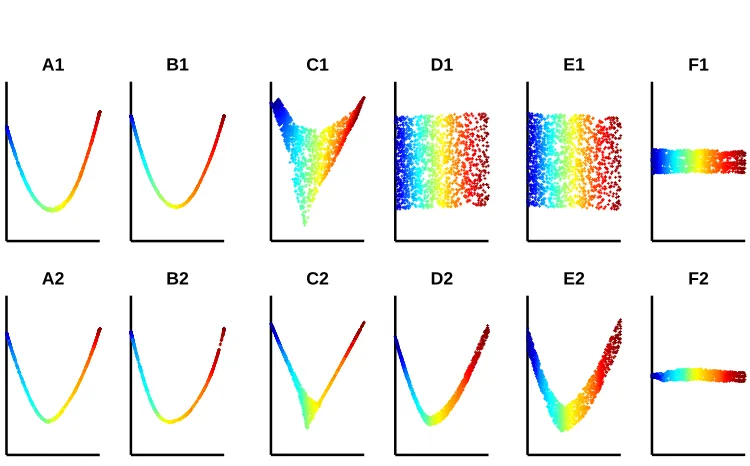
The first data set is a 1600-point sample from the swissroll as obtained from Wittman (retrieved Jan. 2007). The results for the swissroll are given in Fig. 7, A1-F1. The results for the same swissroll, after its first dimension was stretched by a factor 3, are given in Fig. 7, A2-F2. The

original and stretched swissrolls are presented in Fig. 6A. The results for K=8 are given in Fig. 7.

We also checked for K=12,16; but “short-circuits” occur (see Balasubramanian et al., 2002, for a

definition and discussion of “short-circuits”).

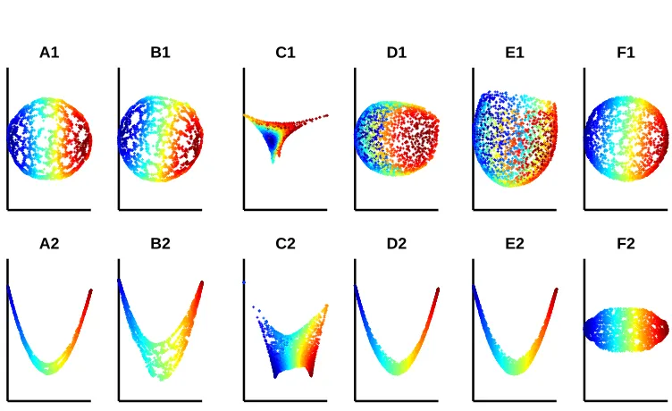
The second data set consists of 2400 points, uniformly sampled from a “fishbowl”, where a “fishbowl” is a two-dimensional sphere minus a neighborhood of the northern pole (see Fig. 6B

for both the “fishbowl” and its stretched version). The results for K=8 are given in Fig. 8. We

also checked for K =12,16; the results are roughly similar. Note that the “fishbowl” is a

two-dimensional manifold embedded inR3_{, which is not an isometry.}

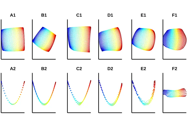
The third data set consists of 900 images of the globe, each of 100_×100 pixels (see Fig. 6C).

The images, provided by Hamm et al. (2005), were obtained by changing the globe’s azimuthal and

elevation angles. The parameters of the variations are given by a 30_×30 array that contains₋45 to

60/−45 60/−41.9 60/−38.79 60/−35.69 60/−32.59 60/−29.48

56.9/−45 56.9/−41.9 56.9/−38.79 56.9/−35.69 56.9/−32.59 56.9/−29.48

53.79/−45 53.79/−41.9 53.79/−38.79 53.79/−35.69 53.79/−32.59 53.79/−29.48

50.69/−45 50.69/−41.9 50.69/−38.79 50.69/−35.69 50.69/−32.59 50.69/−29.48

A

B

C

Figure 6: The data sets for the first example appear in panel A. In the left appears the 1600-point original swissroll and in the right appears the same swissroll, after its first dimension was stretched by a factor of 3. The data for the second example appear in panel B. In the left appears a 2400-point uniform sample from the “fishbowl”, and in the right appears the same “fishbowl”, after its first dimension was stretched by a factor of 4. In panel C

appears the upper left corner of the array of 100_×100 pixel images of the globe. Above

each image we write the elevation and azimuth.

entire set of images and on a strip of 30_×10 angular variations. The results for K=8 are given in

A1 B1 C1 D1 E1 F1

A2 B2 C2 D2 E2 F2

Figure 7: The output of LEM on 1600 points sampled from a swissroll is presented in A1. The output of LEM on the same swissroll after stretching its first dimension by a factor of 3 is presented in A2. Similarly, the outputs of DFM, LLE, LTSA, HLLE, and Isomap

are presented in B1-2, C1-2, D1-2, E1-2, and F1-2, respectively. We used K=8 for all

algorithms except DFM, where we usedσ=2.

These three examples, in addition to the noisy version of the two-dimensional strip discussed in Section 3 (see Fig. 1), clearly demonstrate that when the aspect ratio is sufficiently large, all the normalized-output algorithms prefer to collapse their output.

6. Asymptotics

In the previous sections we analyzed the phenomenon of global distortion obtained by the normalized-output algorithms on a finite input sample. However, it is of great importance to explore the limit behavior of the algorithms, that is, the behavior when the number of input points tends to infinity. We consider the question of convergence in the case of input that consists of a d-dimensional

man-ifold embedded inRD_{, where the manifold is isometric to a convex subset of Euclidean space. By}

convergence we mean recovering the original subset ofRd _{up to a non-singular affine}

transforma-tion.

A1 B1 C1 D1 E1 F1

A2 B2 C2 D2 E2 F2

Figure 8: The output of LEM on 2400 points sampled from a “fishbowl” is presented in A1. The output of LEM on the same “fishbowl” after stretching its first dimension by a factor of 4 is presented in A2. Similarly, the outputs of DFM, LLE, LTSA, HLLE, and Isomap

are presented in B1-2, C1-2, D1-2, E1-2, and F1-2, respectively. We used K=8 for all

algorithms except DFM, where we usedσ=2.

are classes of manifolds on which the normalized-output algorithms cannot be expected to recover the original sample, not even asymptotically.

6.1 LEM and DFM

Let x1,x2, . . . be a uniform sample from the two-dimensional strip S= [0,L]_×[0,1]. Let Xn=

[x1, . . . ,xn]0be the sample of size n. Let K=K(n)be the number of nearest neighbors. Then when

Kn there exists with probability one an N, such that for all n>N the assumptions of Corollary 5.2

hold. Thus, if L>4 we do not expect either LEM or DFM to recover the structure of the strip as

the number of points in the sample tends to infinity. Note that this result does not depend on the number of neighbors or the width of the kernel, which can be changed as a function of the number

of points n, as long as Kn. Hence, we conclude that LEM and DFM generally do not converge,

regardless of the choice of parameters.

A1 B1 C1 D1 E1 F1

A2 B2 C2 D2 E2 F2

Figure 9: The output of LEM on the 30_×30 array of the globe rotation images is presented in A1;

the output of LEM on the array of 30_×10 is presented in A2. Similarly, the outputs of

DFM, LLE, LTSA, HLLE, and Isomap are presented in B1-2, C1-2, D1-2, E1-2, and F1-2

respectively. We used K=8 for all algorithms except DFM, where we choseσto be the

root of the average distance between neighboring points.

operator. Thus, taking a close look at the eigenfunctions of the continuous Laplacian operator may reveal some additional insight into the behavior of both LEM and DFM.

Our working example is the two-dimensional strip S= [0,L]_×[0,1], which can be considered as

the continuous counterpart of the grid X defined in Section 4. Following Coifman and Lafon (2006)

we impose the Neumann boundary condition (see details therein). The eigenfunctions ϕi,j(x1,x2)

and eigenvaluesλi,j on the strip S under these conditions are given by

ϕi,j(x1,x2) =cos _iπ

Lx1

cos(jπx2) λi,j= _iπ

L

2

+ (jπ)2 for i,j=0,1,2, . . . .

When the aspect ratio of the strip satisfies L>M_∈N_{, the first M non-trivial eigenfunctions are}

ϕi,0, i=1, . . . ,M, which are functions only of the first variable x1. Any embedding of the strip based on the first M eigenfunctions is therefore a function of only the first variable x1. Specifically,

whenever L>2 the two-dimensional embedding is a function of the first variable only, and therefore

clearly cannot establish a faithful embedding of the strip. Note that here we have obtained the same

ratio constant L>2 computed for the grid (see Section 4 and Figs. 4 and 5) and not the looser

As mentioned in the beginning of this section, Huo and Smith (2006) proved the convergence of the LTSA algorithm. The authors of HLLE proved that the continuous manifold can be recovered by finding the null space of the continuous Hessian operator (see Donoho and Grimes, 2004, Corollary). However, this is not a proof that the algorithm HLLE converges. In the sequel, we try to understand the relation between Corollary 5.2 and the convergence proof of LTSA.

Let x1,x2, . . .be a sample from a compact and convex domainΩinR2_{. Let Xn= [x1, . . . ,xn]}0 _be

the sample of size n. Letψbe an isometric mapping fromR2_toRD_{, where}

D

the input for the algorithms. We assume that there is an N such that for all n>N the assumptions

of Corollary 5.2 hold. This assumption is reasonable, for example, in the case of a uniform sample from the strip S. In this case Corollary 5.2 states thatΦ(Zn)<Φ(Yn)whenever

4 1+|n0| n

carmax,2 n

√ 2 ¯e(n2)

! <cn,

where cnis the ratio between the variance of Xn(1)and Xn(2)assumed to converge to a constant c. The

expression |n0|

n is the fraction of neighborhoods Xi,nsuch that X

(1)

i,n is located on both sides of zero.

rmax,n is the maximum radius of neighborhood in n0. Note that we expect both |n_n0| and rmax,n to

be bounded whenever the radius of the neighborhoods does not increase. Thus, Corollary 5.2 tells

us that if{e¯(n2)}is bounded from below, we cannot expect convergence from LLE, LTSA or HLLE

when c is large enough.

The consequence of this discussion is that a necessary condition for the convergence of LLE, LTSA and HLLE is that_{e¯(n2)}(and hence, from the assumptions of Corollary 5.2, also{e¯(n1)})

con-verges to zero. If the two-dimensional manifoldψ(Ω)is not contained in a linear two-dimensional

subspace ofRD_{, the mean error ¯e}(_n2)_{is typically not zero due to curvature. However, if the radii}

of the neighborhoods tend to zero while the number of points in each neighborhood tends to

infin-ity, we expect ¯e(n2)→0 for both LTSA and HLLE. This is because the neighborhood matrices Wi

are based on the linear approximation of the neighborhood as captured by the neighborhood SVD. When the radius of the neighborhood tends to zero, this approximation gets better and hence the error tends to zero. The same reasoning works for LLE, although the use of regularization in the

second step of LLE may prevent ¯e(n2)from converging to zero (see Section 2).

We conclude that a necessary condition for convergence is that the radii of the neighborhoods tend to zero. In the presence of noise, this requirement cannot be fulfilled. Assume that each input

point is of the formψ(xi) +εi whereεi∈RD is a random error that is independent ofεj for j6=i.

We may assume thatεi∼N(0,α2I), whereαis a small constant. If the radius of the neighborhood

is smaller thanα, the neighborhood cannot be approximated reasonably by a two-dimensional

pro-jection. Hence, in the presence of noise of a constant magnitude, the radii of the neighborhoods cannot tend to zero. In that case, LLE, LTSA and HLLE might not converge, depending on the ratio c. This observation seems to be known also to Huo and Smith (2006), who wrote:

“... we assumeα=o(r); that is, we have α_{r →}0, as r_→0.

somewhat nonstandard, since the magnitude of the errors is assumed to depend on n,

but it seems to be necessary to ensure the consistency of LTSA.”2

Summarizing, convergence may be expected when n_→∞, if no noise is introduced. If noise is

introduced and ifσ/τis large enough (depending on the level of noiseα), convergence cannot be

expected (see Fig. 1).

7. Concluding Remarks

In the introduction to this paper we posed the following question: Do the normalized-output al-gorithms succeed in revealing the underlying low-dimensional structure of manifolds embedded in high-dimensional spaces? More specifically, does the output of the normalized-output algorithms resemble the original sample up to affine transformation?

The answer, in general, is no. As we have seen, Theorem 5.1 and Corollary 5.2 show that there are simple low-dimensional manifolds, isometrically embedded in high-dimensional spaces, for which the normalized-output algorithms fail to find the appropriate output. Moreover, the dis-cussion in Section 6 shows that when noise is introduced, even of small magnitude, this result holds asymptotically for all the normalized-output algorithms. We have demonstrated these results numerically for four different examples: the swissroll, the noisy strip, the (non-isometrically em-bedded) “fishbowl”, and a real-world data set of globe images. Thus, we conclude that the use of the normalized-output algorithms on arbitrary data can be problematic.

The main challenge raised by this paper is the need to develop manifold-learning algorithms that have low computational demands, are robust against noise, and have theoretical convergence guarantees. Existing algorithms are only partially successful: normalized-output algorithms are efficient, but are not guaranteed to converge, while Isomap is guaranteed to converge, but is com-putationally expensive. A possible way to achieve all of the goals simultaneously is to improve the existing normalized-output algorithms. While it is clear that, due to the normalization constraints, one cannot hope for geodesic distances preservation nor for neighborhoods structure preservation, success as measured by other criteria may be achieved. A suggestion of improvement for LEM appears in Gerber et al. (2007), yet this improvement is both computationally expensive and lacks a rigorous consistency proof. We hope that future research finds additional ways to improve the existing methods, given the improved understanding of the underlying problems detailed in this paper.

Acknowledgments

We are grateful to the anonymous reviewers of present and earlier versions of this manuscript for their helpful suggestions. We thank an anonymous referee for pointing out errors in the proof of Lemma 3.1. We thank J. Hamm for providing the database of globe images. This research was supported in part by Israeli Science Foundation grant and in part by NSF, grant DMS-0605236.

This section contains detailed proofs of Equations 4 and 7, Lemmas 3.1 and A.2, and Theorem 5.1. It also contains discussions regarding the equivalence of the normalized-output algorithms’

repre-sentations, and the estimation of F(K)andF(K)e for a ball of radius r (see Section 4).

A.1 The Equivalence of the Algorithms’ Representations

For LEM, note that according to our representation, one needs to minimize

Φ(Y) =

N

∑

i=1

kWiYik2F = N

∑

i=1

K

∑

j=1

wi,jkyi−yi,jk2,

under the constraints Y0D1=0 and Y0DY =I. Define ˆwrs=wr,j if s is the j-th neighbor of r and

zero otherwise. Define ˆD to be the diagonal matrix such that drr=∑Ns=1wˆrs; note that ˆD=D. Using

these definitions, one needs to minimizeΦ(Y) =∑_r,swˆrskyr−ysk2under the constraints Y0D1ˆ =0

and Y0DYˆ =I, which is the the authors’ representation of the algorithm.

For DFM, as for LEM, we define the weights ˆwrs. Define the N×N matrix ˆW = (wˆrs). Define

the matrix D−1W ; note that this matrix is a Markovian matrix and that vˆ (0)_≡1 is its eigenvector

corresponding to eigenvalue 1, which is the largest eigenvalue of the matrix. Let v(p), p=1, . . . ,d

be the next d eigenvectors, corresponding to the next d largest eigenvaluesλp, normalized such that

v(p)0Dv(p)=1. Note that the vectors v(0), . . . ,v(d)are also the eigenvectors of I₋D−1W correspond-ing to the d+1 lowest eigenvalues. Thus, the matrix[v(1)_{, . . . ,v}(d)_{](up to rotation) can be computed}

by minimizing tr(Y0(D₋W)Y) under the constraints Y0DY =I and Y0D1=0. Simple

compu-tation shows (see Belkin and Niyogi, 2003, Eq. 3.1) that tr(Y0_{(D−W)Y) =} 1

2∑r,swˆrskyr−ysk2.

We already showed that Φ(Y) = ∑r,swˆrskyr−ysk2. Hence, minimizing tr(Y0(D−W)Y) under

the constraints Y0DY =I and Y0D1=0 is equivalent to minimizing Φ(Y) under the same

con-straints. The embedding suggested by Coifman and Lafon (2006) (up to rotation) is the matrix

λ1 v(1)

kv(1)_k, . . . ,λd v(d)

kv(d)_k

. Note that this embedding can be obtained from the output matrix Y by a

simple linear transformation.

For LLE, note that according to our representation, one needs to minimize

Φ(Y) =

N

∑

i=1

kWiYik2_F = N

∑

i=1 kyi−

K

∑

j=1

wi,jyi,jk2

under the constraints Y01=0 and Cov(Y) =I, which is the minimization problem given by Roweis

and Saul (2000).

The representation of LTSA is similar to the representation that appears in the original paper,

differing only in the weights’ definition. We defined the weights Wi following Huo and Smith

(2006), who showed that both definitions are equivalent.

For HLLE, note that according to our representation, one needs to minimize

Φ(Y) =

N

∑

i=1

kWiYik2F= N

∑

i=1

tr Y_i0H_i0HiYi

under the constraint Cov(Y) =I. This is equivalent (up to a multiplication byp(N)) to minimizing

of the algorithm. This minimization can be calculated by finding the d+1 lowest eigenvectors of

H

A.2 Proof of Lemma 3.1

We begin by estimatingΦ(Ye).

Φ(Ye) =

N

∑

i=1

kWiYi+εWiEik2F = N

∑

i=1

K

∑

j=0

Wiyi,j+εWiei,j 2 (14) ≥ N

∑

i=1

K

∑

j=0

Wiyi,j 2

−2ε|(Wiyi,j)0Wiei,j|

≥

N

∑

i=1

K

∑

j=0

(1₋ε)Wiyi,j 2

−εWiei,j 2

= (1₋ε)

N

∑

i=1

kWiYik2F−ε N

∑

i=1

kWiEik2F

≥ (1₋ε)Φ(Y)₋ε

N

∑

i=1

kWik2FkEik2F ,

where ei,jdenotes the j-th row of Ei.

We bound_kWik2F for each of the algorithms by a constant Ca. It can be shown that for LEM and

DFM, Ca≤2K; for LTSA, Ca≤K; for HLLE Ca≤d(d₂+1). For LLE in the case of positive weights

wi,j, we have Ca≤2. Thus, substituting Cain Eq. 14, we obtain

Φ(Ye) _≥ (1₋ε)Φ(Y)₋εCa N

∑

i=1

K

∑

j=0

ei,j

2

≥ (1₋ε)Φ(Y)₋εCaSkEk2_F = (1−ε)Φ(Y)−εCaS.

The last inequality holds true since S is the maximum number of neighborhoods to which a single observation belongs.

A.3 Proof of Equation 4

By definitionσ2=Var(X(1)_{)and hence,}

σ2 ₌ 1 N

m

∑

i=−m q

∑

j=−q

x(_{i j}1)2

= 1

(2m+1)(2q+1)

m

∑

i=−m q

∑

j=−q

i2

= 2

2m+1

m

∑

i=1 i2

= 2

2m+1

(2m+1)(m+1)m 6

= (m+1)m

A.4 Estimation of F(K)andF(K)e for a Ball of Radius r

Calculation ofφ(Yi j)for general K can be different for different choices of neighborhoods.

There-fore, we restrict ourselves to estimatingφ(Yi j)when the neighbors are all the points inside an r-ball

in the original grid. Recall thatφ(Yi j)for an inner point is equal to the sum of the squared distance

between yi jand its neighbors. The function

f(x1,x2) =

_x1

σ

2 +x2

τ

2

agrees with the squared distance for points on the grid, where x1and x2indicate the horizontal and

vertical distances from xi jin the original grid, respectively. We estimateφ(Yi j)using integration of

f(x1,x2)on B(r), a ball of radius r, which yields

φ(Yi j)≈

Z

(x21+x22)<r2

f(x1,x2)dx1dx2= πr4

4

1 σ2+

1 τ2

. (15)

Thus, we obtain F(K)_≈ π₄r4.

We estimateφ(Zi j)similarly. We define the continuous version of the squared distance in the

case of the embedding Z by

g(x1,x2) =x21

1 σ2+

4 ρ2

.

Integration yields

φ(Zi j)≈

Z

(x21+x22)<r2

g(x1,x2)dx1dx2= πr4

4

1 σ2+

4 ρ2

. (16)

Hence, we obtain F(K)e _≈ π₄r4 and the relations between Eqs. 5 and 6 are preserved for a ball of

general radius.

For DFM, a general rotation-invariant kernel was considered for the weights. As with Eqs. 15

and 16, the approximations ofφ(Yi j)andφ(Zi j)for the general case with neighborhood radius r are

given by

Z

(x2 1+x22)<r2

f(x1,x2)k(x1,x2)dx1dx2=

 π Z

0<t<r

k(t2_)t3_dt

  1

σ2+ 1 τ2

and

Z

(x2 1+x22)<r2

g(x1,x2)k(x1,x2)dx1dx2=

 π Z

0<t<r

k(t2)t3dt

  1

σ2+ 4 ρ2

.

Note that the ratio between these approximations ofφ(Yi j)andφ(Zi j)is preserved. In light of these

computations it seems that for the general case of rotation-invariant kernels, φ(Yi j)>φ(Zi j) for