A 2D Time Domain DRBEM Computer Model for
Magneto-Thermoelastic Coupled Wave Propagation Problems
Mohamed Abdelsabour Fahmy
1, 2, *1 Mathematics Department, University College, Umm Al-Qura University, Makkah, the Kingdom of Saudi Arabia. 2 Faculty of Computers and Informatics, Suez Canal University, Ismailia, Egypt.
Received 09 September 2013; received in revised form 21 January 2014; accepted 10 March 2014
Abstract
A numerical computer model based on the dual reciprocity boundary element method (DRBEM) is extended to study magneto-thermoelastic coupled wave propagation problems with relaxation times involving anisotropic functionally graded solids. The model formulation is tested through its application to the problem of a solid placed in a constant primary magnetic field acting in the direction of the z-axis and rotating about this axis with a constant angular velocity. In the case of two-dimensional deformation, an implicit-explicit time domain DRBEM was presented and implemented to obtain the solution for the displacement and temperature fields. A comparison of the results is presented graphically in the context of Lord and Shulman (LS) and Green and Lindsay (GL) theories. Numerical results that demonstrate the validity of the proposed method are also presented graphically.
Keywords: magneto-thermo-elasticity, relaxation times, anisotropic, functionally graded solid, dual reciprocity boundary element method
1.
Introduction
The dynamical interaction between the thermal and mechanical fields in anisotropic materials has great practical applications in modern aeronautics, astronautics, earthquake engineering, soil dynamics, mining engineering, nuclear reactors and high-energy particle accelerators, for instance. Lord and Shulman [1] developed the theory of generalized thermoelasticity with one relaxation time by constructing a new law of heat conduction to replace the classical Fourier's law. This law contains the heat flux vector as well as its time derivative. It contains also new constant that acts as relaxation time. Since the heat equation of this theory is the wave-type, it automatically ensures finite speeds of propagation for heat and elastic waves. Green and Lindsay [2] included a temperature rate among the constitutive variables to develop a temperature– rate-dependent thermoelasticity that does not violate the classical Fourier's law of heat conduction when the body under consideration has a center of symmetry; this theory also predicts a finite speed of heat propagation and is known as the theory of thermoelasticity with two relaxation times. According to these theories, heat propagation should be viewed as a wave phenomenon rather than diffusion one. Relevant theoretical developments on the subject were made by Green and Naghdi [3, 4], they developed three models for generalized thermoelasticity of homogeneous isotropic materials which are labeled as model I, II and III. These theories of thermoelasticity Lord and Shulman (LS), Green and Lindsay (GL) and Green and Naghdi (GN) theories are known as the generalized theories of thermoelasticity with finite thermal wave speed. It is hard to find the analytical solution of magneto-thermoelasticity problem in a general case, therefore, an important number of
engineering and mathematical papers devoted to the numerical solution have studied the overall behavior of such materials (Das and Kanoria [5]; Huacasi et al. [6]; Paulino and Kim [7]; Abd-Alla et al. [8-10]; Fahmy [11-16]; Fahmy and El-Shahat [17]; Han and Hong [18]; Xiong and Tian [19]).
The first step of the boundary element method (BEM) is the transformation of the physical problem at hand to an integral equation. The latter is defined frequently solely on the boundary, in which case the dimensionality of the problem is reduced by one. The presence of domain integrals in the BEM formulation implies domain discretization and this makes the BEM inefficient when compared with domain discretization techniques such as finite element method (FEM) or finite difference method (FDM). Thus, many efforts have been made to convert the domain integral into a boundary one (Marin et al. [20]; Wen and Khonsari [21]; Javaran et al. [22]). One of the most widely used techniques to accomplish this task is the dual reciprocity boundary element method (DRBEM) developed by Nardini and Brebbia [23] in the context of two-dimensional (2D) elastodynamics and has been extended to deal with a variety of problems wherein the domain integral may account for linear-nonlinear static-dynamic effects (Brebbia et al. [24]; Wrobel and Brebbia [25]; Partridge and Brebbia [26]; Partridge and Wrobel [27]; Partridge et al. [28]; El-Naggar et al. [29, 30]; Gaul et al.[31]; Fahmy [32-34]).
The main purpose of this work is to study the generalized magneto-thermoelastic coupled wave propagation problems with relaxation times in anisotropic functionally graded solid placed in a constant primary magnetic fieldacting in the direction of the z-axis and rotating about this axis with a constant angular velocity. An implicit-explicit time integration procedurewas developed and implemented for use with the dual reciprocity boundary element method (DRBEM) to obtain the solution for the governing equations of the considered problem. A comparison of the results is presented graphically in the context of LS and GL theories. Numerical results that demonstrate the validity of the proposed method are also presented graphically.
2.
Formulation of the Problem
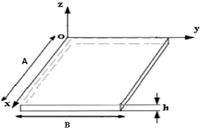
Consider a Cartesian coordinates system as shown in Fig. 1, we shall consider a functionally graded anisotropic solid placed in a primary magnetic field acting in the direction of the -axis and rotating about it with a constant angular velocity. The solid occupies the region , the material properties are assumed to be graded through the direction. Here we address the generalized twodimensional deformation problem in -plane only.We also consider the following variant form of the power law material model , where is a dimensionless constant.
Fig. 1 The coordinate system of the solid
(1)
(2)
(3)
(4)
3.
Numerical Implementation
Making use of (2) and (3), we can write (1) as follows: (5)where (6) The field equations can now be written in operator form as follows, (7)
(8)
where the operators and are defined in equation (5), and the operators and are defined as follows: (9)
(10)
Using the weighted residual method (WRM), the differential equation (7) is transformed into an integral equation (11)
Now, we choose the fundamental solution as weighting function as follows, (12)
The corresponding traction field can be written as (13)
Applying integration by parts to (11) using the sifting property of the Dirac distribution, with (12) and (14), we can write the following elastic integral representation formula
(15)
The fundamental solution of the thermal operator , defined by
(16)
By implementing the WRM and integration by parts, the differential equation (8) is transformed into the thermal reciprocity equation
(17)
where the heat fluxes are independent of the elastic field and can be expressed as follows:
(18)
(19)
By the use of sifting property, we obtain from (17) the thermal integral representation formula
(20)
The integral representation formulae of elastic and thermal fields (15) and (20) can be combined to form a single equation as follows,
(21)
It is convenient to use the contracted notation to introduce generalized thermoelastic vectors and tensors, which contain corresponding elastic and thermal variables as follows:
(22)
(23)
(24)
(25)
The thermoelastic representation formula (21) can be written in contracted notation as:
(27)
The vector can be written in the split form as follows: (28)
where (29)
(30)
with (31)
(32)
(33)
(34)
(35)
The thermoelastic representation formula (21) can also be written in matrix form as follows:
(36) Our task now is to implement the DRBEM. To transform the domain integral in (27) to the boundary, we approximate the source vector in the domain as usual by a series of given tensor functions and unknown coefficients
(37)
According to the DRBEM, the surface of the solid has to be discretized into boundary elements. In order to make the implementation easy to compute, we use collocation points on the boundary and another in the interior of so that the total number of interpolation points is .
Thus, the thermoelastic representation formula (27) can be written in the following form,
By applying the WRM to the following inhomogeneous elastic and thermal equations:
(39)
(40)
The elastic and thermal representation formulae are as follows (Fahmy [35]),
(41)
(42)
The dual representation formulae of elastic and thermal fields can be combined to form a single equation as follows,
(43)
With the substitution of (43) into (38), the dual reciprocity representation formula of coupled thermoelasticity can be expressed as follows,
(44)
To calculate interior stresses, (44) is differentiated with respect to as follows,
(45)
According to the steps described in Fahmy [36], the dual reciprocity boundary integral equation (44) can be written in the following system of equations:
(46)
The technique was proposed by Partridge et al. [27] can be extended to treat the convective terms, then the generalized displacements and velocities are approximated by a series of tensor functions and unknown coefficients and
(47)
The gradients of the generalized displacement and velocity can be approximated as follows,
(49)
(50)
These approximations are substituted into equations (30) and (34) to approximate the corresponding source terms as follows,
(51)
(52)
where
(53)
(54)
The same point collocation procedure described in Gaul, et al. [31] can be applied to (37), (47) and (48). This leads to the following system of equations,
(55)
Similarly, the application of the point collocation procedure to the source terms equations (31), (32), (33), (35), (51) and (52) leads to the following system of equations:
with (56)
(57)
(58)
(59)
(60)
(61)
Solving the system (55) for , and yields
Now, the coefficients can be expressed in terms of nodal values of the unknown displacements , velocities and
accelerations as follows:
(63) where and are assembled using the submatrices and respectively.
Substituting from Eq. (63) into Eq. (46), we obtain (Fahmy [37])
(64)
in which and are independent of time and are defined by
(65)
where , and represent the volume, mass, damping and stiffness matrices, respectively; and represent the
acceleration, velocity, displacement and external force vectors, respectively. The initial value problem consists of finding the function satisfying equation (64) and the initial conditions where are given vectors of initial data. Then, from Eq. (78), we can compute the initial acceleration vector as follows (Prevost and Tao [38])
(66)
An implicit-explicit time integration algorithm of Hughes and Liu [39, 40] was presented and implemented for use with the DRBEM. This algorithm consists of satisfying the following equations
(67)
(68)
(69)
where
(70)
(71)
in which the implicit and explicit parts are respectively denoted by the superscripts and . Also, we used the quantities and to denote the predictor values, and and to denote the corrector values. It is easy to recognize that
the equations (68)-(71) correspond to the Newmark formulas (Newmark [41]).
At each time-step, equations (67)-(71), constitute an algebraic problem in terms of the unknown . The first step in
the code starts by forming and factoring the effective mass
The time step must be constant to run this step. As the time-step is changed, the first step should be repeated at each new step. The second step is to form residual force
(73)
Note that in the implicit part, is always non-symmetric. However, still possesses the usual "band-profile" structure associated with the connectivity of the DRBEM mesh, and has a symmetric profile. So the third step is to solve using a Crout elimination algorithm (Taylor [42]) which fully exploits that structure in that zeroes outside the profile are neither stored nor operated upon. The fourth step is to use predictor-corrector equations (68) and (69) to obtain the corrector displacement and velocity vectors, respectively.
4.
Numerical Results and Discussion
Following Rasolofosaon and Zinszner [43] monoclinic North Sea sandstone reservoir rock was chosen as an anisotropic material and physical data are as follows: Elasticity tensor GPa (74) Mechanical temperature coefficient N/K (75) Tensor of thermal conductivity is (76)Mass density ρ= 2216 kg/m3 and heat capacity J/(kg K), Oersted, Gauss/Oersted, , . The numerical values of the temperature and displacement are obtained by discretizing the boundary into 120 elements and choosing 60 well spaced out collocation points in the interior of the solution domain, refer to the recent work of Fahmy [44-46]. The initial and boundary conditions considered in the calculations are at (77)
at (78)
at (79)
at (80)
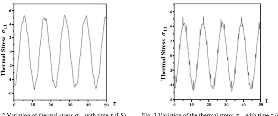
Figures 2 and 3 show the variation of the temperature with time . We can conclude from these figures that the maximum temperature occurs at in the LS theory, but it occurs at in the GL theory. It is seen also from these figures that the oscillation period in the GL is less than the oscillation period in LS theory.
Fig. 2 Variation of thermal stress with time (LS) Fig. 3 Variation of the thermal stress with time (GL)
Figures 4 and 5 show the variation of the displacement with time . It may be seen from these figures that the displacement appears to have an intense oscillation. The oscillation period of LS theory is less than the oscillation period of GL theory. It can be seen that the maximum displacement occurs at for the LS theory, but it occurs at for the GL theory. The minimum magnitude of displacement occurs at homogeneous case.
Fig. 4 Variation of the thermal stress with time (LS) Fig. 5 Variation of the thermal stress with time (GL)
Figures 6 and 7 illustrate the variation of the displacement with time . It may be seen from these figures that the displacement appears to have an intense oscillation. The oscillation period of LS theory is less than the oscillation period of GL theory. It can be seen from these figures that the maximum displacement occurs at for the LS theory. But it occurs at for the GL theory.
Figures 2-7 show the difference between the LS and GL theories for the thermal stresses , and at .
We can see also from these figures that the thermal sresses appear in an intense oscillation.
Figures 2 and 3 illustrate the variation of the thermal stress with time . It can be seen that the maximum thermal
stress occurs at for the LS theory. But it occurs at for the GL theory.
Figures 4 and 5 show the variation of the thermal stress with time . It can be seen that the maximum thermal
stress occurs at for the LS theory. But it occurs at for the GL theory.
Figures 6 and 7 illustrate the variation of the thermal stress with time . It can be seen that the maximum thermal
stress occurs at for the GL theory. But it occurs at for the LS theory.
It can be noted from these figures that the maximum thermal stress occurs in GL theory. It is seen also from these figures that the oscillation period of LS theory is less than the oscillation period of GL theory for the thermal stresses and
. But the oscillation period of GL theory is less than the oscillation period of LS theory for the thermal stress .
The present work should be applicable to any dynamic coupled magneto-thermoelastic deformation problem. The proposed technique in the present study was discussed in the context of the viscoelastic problems in Fahmy [47, 48] and discussed in the context of the generalized theories of thermoelasticity in Fahmy et al. [49-52]. The example considered by Mojdehi et al. [53], may be also considered as a special case of the current general study. Also, there are a lot of practical applications may be deduced as special cases from this general study and may be implemented in commercial finite element method (FEM) software packages FlexPDE 6.
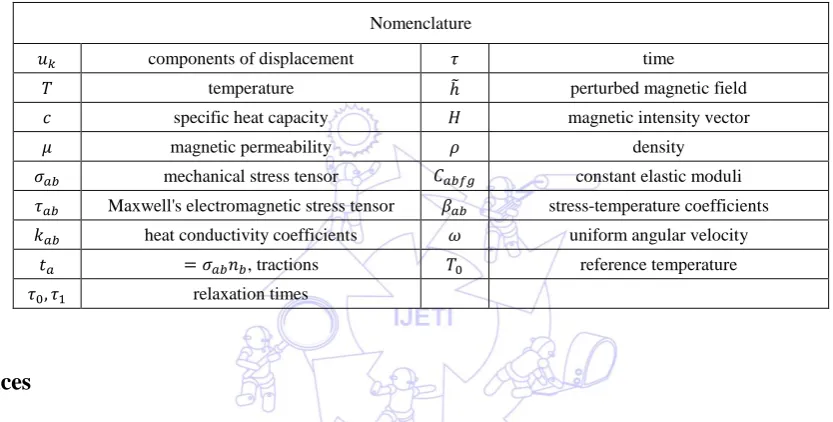
In the special case under consideration, the results are plotted in figures 8-10 to show the validity of the DRBEM. These results obtained with the DRBEM have been compared graphically with those obtained using the Meshless Local Petrov-Galerkin (MLPG) method of Mojdehi et al. [53] and also the results obtained from the FlexPDE 6 are shown graphically in the same figures to confirm the validity of the proposed method. It can be seen from these figures that the DRBEM resultsare in excellent agreement with the results obtained by MLPG and FEM, thus confirming the accuracy of the DRBEM.
Fig. 9 Variation of the displacement u1 with time for three methods: DRBEM, MLPG and FEM
Fig. 10 Variation of the displacement u2 with time for three methods: DRBEM, MLPG and FEM
Nomenclature
components of displacement time
temperature perturbed magnetic field
specific heat capacity magnetic intensity vector
magnetic permeability density
mechanical stress tensor constant elastic moduli
Maxwell's electromagnetic stress tensor stress-temperature coefficients
heat conductivity coefficients uniform angular velocity
, tractions reference temperature
relaxation times
References
[1] H. W. L d and Y. S ulman, “A g n al z d dynam cal y f m la c y,” J u nal f M c an c and Physics of Solids, vol. 15, pp. 299-309, 1967.
[2] A. E. G n and K. A. L nd ay, “T m la c y,” J u nal f Ela c y, v l. 2, no. 1, pp. 1-7, 1972.
[3] A. E. Green and P. M. Naghdi, “On undamped a av n an la c l d,” Journal of Thermal Stresses, vol. 15, no. 2, pp. 253-264, 1992.
[4] A. E. Green and P. M. Naghdi, “Thermoelasticity u n gy d pa n,” Journal of Elasticity, vol. 31, pp. 189-208, 1993.
[5] P. Das and M. Kanoria,“Magneto-thermo-elastic response in a perfectly conducting medium with three-phase-lag effect,” Acta Mechanica, vol. 223, pp. 811-828, 2012.
[6] W. Huacasi, W. J. Mansur, and J. P. S. Azevedo, “A novel hypersingular B.E.M. formulation for three-dimensional p n al p bl m ,” Journal of Brazilian Society of Mechanical Sciences and Engineering, vol. 25, pp. 364-372, 2003. [7] G. H. Paulino and J. H. Kim, “The weak patch test for nonhomogeneous materials model d g ad d f n l m n ,”
Journal of Brazilian Society of Mechanical Sciences and Engineering, vol. 29, pp. 63-81, 2007.
[8] A. M. Abd-Alla, A. M. El-Naggar and M. A. Fahmy, “Magneto-thermoelastic problem in non-homogeneous isotropic cyl nd ,” Heat and Mass transfer, vol. 39, pp. 625-629, 2003.
[9] A. M. Abd-Alla, M. A. Fahmy and T. M. El-Shahat, “Magneto-thermo-elastic stresses in inhomogeneous anisotropic solid n p nc f b dy f c ,” Far East Journal of Applied Mathematics, vol. 27, pp. 499-516, 2007.
[10] A. M. Abd-Alla, M. A. Fahmy and T. M. El-Shahat, “Magneto-thermo-elastic problem of a rotating non-homogeneous an p c l d cyl nd ,”Archive of Applied Mechanics, vol. 78, pp. 135-148, 2008.
[12] M. A. Fahmy, “Thermoelastic stresses in a rotating non- m g n u an p c b dy,” Numerical Heat Transfer, Part A: Applications, vol. 53, pp. 1001-1011, 2008.
[13] M. A. Fahmy, “Thermal stresses in a spherical shell under three m la c m d l u ng FDM,” International Journal of Numerical Methods and Applications, vol. 2, pp. 123-128, 2009.
[14] M. A. Fahmy, “Finite difference algorithm for transient magneto-thermo-elastic stresses in a non-homogeneous solid cyl nd ,” International Journal of Materials Engineering and Technology, vol. 3, pp. 87-93, 2010.
[15] M. A. Fahmy, “A time-stepping DRBEM for magneto-thermo-viscoelastic interactions in a rotating nonhomogeneous anisotrop c l d,” International Journal of Applied Mechanics, vol. 3, pp. 1-24, 2011.
[16] M. A. Fahmy, “Numerical modeling of transient magneto-thermo-viscoelastic waves in a rotating nonhomogeneous anisotr p c l d und n al ,” International Journal of Modeling, Simulation and Scientific Computing, vol. 3, pp. 125002, 2012.
[17] M. A. Fahmy and T. M. El-Shahat, “The effect of initial stress and inhomogeneity on the thermoelastic stresses in a a ng an p c l d,” Archive of Applied Mechanics, vol. 78, pp. 431-442, 2008.
[18] Y. Han and W. Hong, “Coupled magnetic field and viscoelasticity of ferrogel,” International Journal of Applied Mechanics, vol. 3, pp. 259-278, 2011.
[19] Q. L. Xiong and X. G. Tian,“Transient magneto-thermoelastic response for a semi-infinite body with voids and variable material properties during thermal shock,” International Journal of Applied Mechanics, vol. 3, pp. 881-902, 2011. [20] L. Marin, L. Elliott, P. J. Heggs, D. B. Ingham, D. Lesnic and X. Wen, “Dual reciprocity boundary element method
solution of the Cauchy problem for Helmholtz-type equat n va abl c ff c n ,” Journal of Sound and Vibration, vol. 297, pp. 89-105, 2006.
[21] J. Wen and M. M. Khonsari, “Transient heat conduction in rolling/sliding components by a dual reciprocity boundary element method,” International Journal of Heat and Mass Transfer, vol. 52, pp. 1600-1607, 2009.
[22] S. H. Javaran, N. Khaji and A. Noorzad, “First kind Bessel function (J-Bessel) as radial basis function for plane dynamic analysis using dual reciprocity boundary element method,” Acta Mechanica, vol. 218, pp. 247-258, 2011.
[23] D. Nardini and C. A. Brebbia, “A new approach to free vibration analysis using boundary elements,” Applied Mathematical Modelling, vol. 7, pp. 157-162, 1983.
[24] C. A. Brebbia, J. C. F. Telles, and L. Wrobel, Boundary element techniques in engineering. New York: Springer-Verlag, 1984.
[25] L. C. Wrobel and C. A. Brebbia, “The dual reciprocity boundary element formulation f n nl n a d ffu n p bl m ,” Computer Methods in Applied Mechanics and Engineering, vol. 65, pp. 147-164, 1987.
[26] P. W. Partridge and C. A. Brebbia, “Computer implementation of the BEM dual reciprocity method for the solution of g n al f ld qua n ,” Communications Applied Numerical Methods, vol. 6, pp. 83-92, 1990.
[27] P. W. Partridge, C. A. Brebbia and L. C. Wrobel, The dual reciprocity boundary element method. Southampton: Computational Mechanics Publications, 1992.
[28] P. W. Partridge and L. C. Wrobel, “The dual reciprocity boundary element method for spontaneous ignition,” International Journal for Numerical Methods in Engineering, vol. 30, pp. 953-963, 1990.
[29] A. M. El-Naggar, A. M. Abd-Alla, M. A. Fahmy, and S. M. Ahmed, “Thermal stresses in a rotating non-homogeneous orthotropic hollow cylinder,” Heat and Mass Transfer, vol. 39, pp. 41-46, 2002.
[30] A. M. El-Naggar, A. M. Abd-Alla, and M. A. Fahmy, “The propagation of thermal stresses in an infinite elastic slab," Applied Mathematics and Computation, vol. 157, pp. 307-312, 2004.
[31] L. Gaul, M. Kögl, M. Wagner, Boundary element methods for engineers and scientists. Berlin: Springer-Verlag, 2003. [32] M. A. Fahmy, “Application of DRBEM to non-steady state heat conduction in non-homogeneous anisotropic media
under various boundary elements,” Far East Journal of Mathematical Sciences, vol. 43, pp. 83-93, 2010.
[33] M. A. Fahmy, “Influence of inhomogeneity and initial stress on the transient magneto-thermo-visco-elastic stress waves in an anisotropic solid,” World Journal of Mechanics, vol. 1, pp. 256-265, 2011.
[34] M. A. Fahmy, “Transient magneto-thermoviscoelastic plane waves in a non-homogeneous anisotropic thick strip subjected to a moving heat source,” Applied Mathematical Modelling, vol. 36, pp. 4565-4578, 2012.
[35] M. A. Fahmy, “Transient magneto-thermo-elastic stresses in an anisotropic viscoelastic solid with and without moving heat source,” Numerical Heat Transfer, Part A: Applications, vol. 61, pp. 547-564, 2012.
[36] M. A. Fahmy, “A time-stepping DRBEM for the transient magneto-thermo-visco-elastic stresses in a rotating non-homogeneous anisotropic solid,” Engineering Analysis with Boundary Elements, vol. 36, pp. 335-345, 2012. [37] M. A. Fahmy, “The effect of rotation and inhomogeneity on the transient magneto-thermoviscoelastic stresses in an
[38] J. H. Prevost and D. Tao, “Finite element analysis of dynamic coupled thermoelasticity p bl m laxa n m ,” ASME Journal of Applied Mechanics, vol. 50, pp. 817-822, 1983.
[39] T. J. R. Hughes and W. K. Liu, “Implicit-Explicit finite element in Transient analysis: Stability y,” ASME Journal of Applied Mechanics, vol. 45, pp. 371-374, 1978.
[40] T. J. R. Hughes and W. K. Liu, “Implicit-explicit finite element in transient analysis: Implementation and numerical xampl ,” ASME Journal of Applied Mechanics, vol. 45, pp. 375-378, 1978.
[41] N. M. Newmark, “A method of compu a n f uc u al dynam c ,” Journal of the Engineering Mechanics Division, vol. 85, pp. 67-94, 1959.
[42] R. L. Taylor, Computer procedures for finite element analysis. In: Zienckiewicz OC. The finite element method. 3rd ed. London: McGraw Hill, 1977.
[43] P. N. J. Rasolofosaon and B. E. Zinszner, “Comparison between permeability anisotropy and elasticity anisotropy of reservoir rocks,” Geophysics, vol. 67, pp. 230-240, 2002.
[44] M. A. Fahmy,“Implicit-explicit time integration DRBEM for generalized magneto-thermoelasticity problems of rotating anisotropic viscoelastic functionally graded solids,” Engineering Analysis with Boundary Elements, vol. 37, pp. 107-115, 2013.
[45] M. A. Fahmy, “A three-dimensional generalized magneto-thermo-viscoelastic problem of a rotating functionally graded anisotropic solids with and without energy dissipation,” Numerical Heat Transfer. Part A: Applications, vol. 63, pp. 713-733, 2013.
[46] M. A. Fahmy, “Generalized magneto-thermo-viscoelastic problems of rotating functionally graded anisotropic plates by the dual reciprocity boundary element method,” Journal of Thermal Stresses, vol. 36, pp. 284-303, 2013.
[47] M. A. Fahmy,“A 2-D DRBEM for generalized Magneto-Thermo-Viscoelastic Transient Response of rotating
functionally g ad d an p c ck p,” In na nal J u nal f Eng n ng and T c n l gy Inn va n, vol. 3, pp. 70-85, 2013.
[48] M. A. Fahmy, “A computerized DRBEM model for generalized magneto-thermo-visco-elastic stress waves in
functionally graded anisotropic thin film/substrate structures,” Latin American Journal of Solids and Structures, vol. 11, pp. 386-409, 2014.
[49] M. A. Fahmy, A. M. Salem, M. S. Metwally and M. M. Rashid, “Computer implementation of the Drbem for studying the generalized thermoelastic responses of functionally graded anisotropic rotating plates with one relaxation time,” International Journal of Applied Science and Technology, vol. 3, no. 7, pp. 130-140, 2013.
[50] M. A. Fahmy, A. M. Salem, M. S. Metwally and M. M. Rashid, “Computer implementation of the Drbem for studying the classical uncoupled theory of thermoelasticity of functionally graded anisotropic rotating plates,” International Journal of Engineering Research and Applications, vol. 3, no. 6, pp. 1146-1154, 2013.
[51] M. A. Fahmy, A. M. Salem, M. S. Metwally and M. M. Rashid, “Computer implementation of the Drbem for studying the classical coupled Thermoelastic responses of functionally graded anisotropic plates,” Physical Science International Journal, vol. 4, no. 5, pp. 674-685, 2014.
[52] M. A. Fahmy, A. M. Salem, M. S. Metwally and M. M. Rashid, “Computer implementation of the DRBEM for studying the generalized thermo elastic responses of functionally graded anisotropic rotating plates with two relaxation times,” British Journal of Mathematics & Computer Science, vol. 4, no. 7, pp. 1010-1026, 2014.