Learning Theory for Distribution Regression
Zolt´an Szab´o∗ [email protected]
ORCID 0000-0001-6183-7603
Gatsby Unit, University College London Sainsbury Wellcome Centre, 25 Howland Street London - W1T 4JG, UK
Bharath K. Sriperumbudur [email protected]
Department of Statistics Pennsylvania State University University Park, PA 16802, USA
Barnab´as P´oczos [email protected]
Machine Learning Department School of Computer Science Carnegie Mellon University
5000 Forbes Avenue Pittsburgh PA 15213 USA
Arthur Gretton [email protected]
ORCID 0000-0003-3169-7624
Gatsby Unit, University College London Sainsbury Wellcome Centre, 25 Howland Street London - W1T 4JG, UK
Editor:Ingo Steinwart
Abstract
We focus on the distribution regression problem: regressing to vector-valued outputs from probability measures. Many important machine learning and statistical tasks fit into this framework, including multi-instance learning and point estimation problems without ana-lytical solution (such as hyperparameter or entropy estimation). Despite the large number of available heuristics in the literature, the inherent two-stage sampled nature of the prob-lem makes the theoretical analysis quite challenging, since in practice only samples from sampled distributions are observable, and the estimates have to rely on similarities com-puted between sets of points. To the best of our knowledge, the only existing technique with consistency guarantees for distribution regression requires kernel density estimation as an intermediate step (which often performs poorly in practice), and the domain of the distributions to be compact Euclidean. In this paper, we study a simple, analytically com-putable, ridge regression-based alternative to distribution regression, where we embed the distributions to a reproducing kernel Hilbert space, and learn the regressor from the em-beddings to the outputs. Our main contribution is to prove that this scheme is consistent in the two-stage sampled setup under mild conditions (on separable topological domains enriched with kernels): we present an exact computational-statistical efficiency trade-off analysis showing that our estimator is able to match theone-stage sampled minimax op-∗. Now at Applied Mathematics Department, Center for Applied Mathematics, ´Ecole Polytechnique,
timal rate (Caponnetto and De Vito, 2007; Steinwart et al., 2009). This result answers a 17-year-old open question, establishing the consistency of the classical set kernel (Haussler, 1999; G¨artner et al., 2002) in regression. We also cover consistency for more recent kernels on distributions, including those due to Christmann and Steinwart (2010).
Keywords: Two-Stage Sampled Distribution Regression, Kernel Ridge Regression, Mean Embedding, Multi-Instance Learning, Minimax Optimality
1. Introduction
We address the learning problem ofdistribution regression in the two-stage sampled setting, where we only have bags of samples from the probability distributions: we regress from probability measures to real-valued (P´oczos et al., 2013) responses, or more generally to vector-valued outputs (belonging to an arbitrary separable Hilbert space). Many classical problems in machine learning and statistics can be analysed in this framework. On the machine learning side, multiple instance learning (Dietterich et al., 1997; Ray and Page, 2001; Dooly et al., 2002) can be thought of in this way, where each instance in a labeled bag is an i.i.d. (independent identically distributed) sample from a distribution. On the statistical side, tasks might include point estimation of statistics on a distribution without closed form analytical expressions (e.g., its entropy or a hyperparameter).
Intuitive description of our goal: Let us start with a somewhat informal definition of the distribution regression problem and an intuitive phrasing of our goals. Suppose that our data consist of z = {(xi, yi)}li=1, where xi is a probability distribution, yi is its label (in the simplest case yi ∈ R or yi ∈ Rd) and each (xi, yi) pair is i.i.d. sampled from a meta distributionM. However, we do not observexi directly; rather, we observe a sample
xi,1, . . . , xi,Ni
i.i.d.
∼ xi. Thus the observed data are ˆz = {({xi,n}Nn=1i , yi)}li=1. Since xi,j is sampled from xi, and xi is sampled fromM, we call this process two-stage sampling. Our goal is to predict a newyl+1 from a new batch of samplesxl+1,1, . . . , xl+1,Nl+1 drawn from a
new distributionxl+1∼ M. For example, in a medical application, theithpatient might be
identified with a probability distribution (xi), which can be periodically assessed by blood tests ({xi,n}Nn=1i ). We are also given some health indicator of the patient (yi), which might be inferred from his/her blood measurements. Based on the observations (ˆz), we might wish to learn the mapping from the set of blood tests to the health indicator, and the hope is that by observing more patients (largerl) and performing a larger number of tests (larger
Ni) the estimated mapping ( ˆf = ˆf(ˆz)) becomes more “precise”. Briefly, we consider the following questions:
Can the distribution regression problem be solved consistently under mild conditions? What is the exact computational-statistical efficiency trade-off implied by the two-stage sampling?
In our work the estimated mapping ( ˆf) is the analytical solution of a kernel ridge regression (KRR) problem.1 The performance of ˆf depends on the assumed function class (H), the
family of ˆf candidates used in the ridge formulation. We shall focus on the analysis of two settings:
1. Well-specified case (f∗ ∈H): In this case we assume that the regression function
f∗ belongs toH. We focus on bounding the goodness of ˆf compared to f∗. In other words, if R[f∗] denotes the prediction error (expected risk) of f∗, then our goal is to derive a finite-sample bound for the excess risk, E( ˆf , f∗) = R[ ˆf]− R[f∗] that holds with high probability. We make use of this bound to establish the consistency of the estimator (i.e., drive the excess risk to zero) and to derive the exact computational-statistical efficiency trade-off of the estimator as a function of the sample number (l,
N =Ni,∀i) and the problem difficulty (see Theorem 5 and its corresponding remarks for more details).
2. Misspecified case (f∗ ∈L2\H): Since in practise it might be hard to check whether
f∗ ∈H, we also study the misspecified setting of f∗ ∈L2; the relevant case is when
f∗ ∈ L2\H. In the misspecified setting the ’richness’ of H has crucial importance, in other words the size of D2H = inff∈Hkf∗ −fk22, the approximation error from H.
Our main contributions consist of proving a finite-sample excess risk bound, using which we show that the proposed estimator can attain the ideal performance, i.e.,
E( ˆf , f∗)−D2H can be driven to zero. Moreover, on smooth classes of f∗-s, we give a simple and explicit description for the computational-statistical efficiency trade-off of our estimator (see Theorem 9 and its corresponding remarks for more details).
There exist a vast number of heuristics to tackle learning problems on distributions; we will review them in Section 5. However, to the best of our knowledge, the only prior work addressing theconsistency of regression on distributions requires kernel density estimation (P´oczos et al., 2013; Oliva et al., 2014; Sutherland et al., 2016), which assumes that the response variable is scalar-valued,2 and the covariates are nonparametric continuous dis-tributions on Rd. As in our setting, the exact forms of these distributions are unknown;
they are available only through finite sample sets. P´oczos et al. estimated these distribu-tions through a kernel density estimator (assuming these distribudistribu-tions have a density) and then constructed a kernel regressor that acts on these kernel density estimates.3 Using the classical bias-variance decomposition analysis for kernel regressors, they showed the consis-tency of the constructed kernel regressor, and provided a polynomial upper bound on the rates, assuming the true regressor to be H¨older continuous, and the meta distribution that generates the covariates xi to have finite doubling dimension (Kpotufe, 2011).4
One can define kernel learning algorithms on bags based on set kernels (G¨artner et al., 2002) by computing the similarity of the sets/bags of samples representing the input dis-tributions; set kernels are also called called multi-instance kernels or ensemble kernels, and are examples of convolution kernels (Haussler, 1999). In this case, the similarity of two sets
2. Oliva et al. (2013, 2015) consider the case where the responses are also distributions or functions. 3. We would like to clarify that the kernels used in their work are classical smoothing kernels—extensively
studied in non-parametric statistics (Gy¨orfi et al., 2002)—and not the reproducing kernels that appear throughout our paper.
is measured by the average pairwise point similarities between the sets. From a theoretical perspective, nothing is known about the consistency of set kernel based learning method since their introduction in 1999 (Haussler, 1999; G¨artner et al., 2002): i.e. in what sense (and with what rates) is the learning algorithm consistent, when the number of items per bag, and the number of bags, are allowed to increase?
It is possible, however, to view set kernels in a distribution setting, as they represent valid kernels between (mean) embeddings of empirical probability measures into a repro-ducing kernel Hilbert space (RKHS; Berlinet and Thomas-Agnan, 2004). The population limits are well-defined as being dot products between the embeddings of the generating distributions (Altun and Smola, 2006), and for characteristic kernels the distance between embeddings defines a metric on probability measures (Sriperumbudur et al., 2011; Gretton et al., 2012). When bounded kernels are used, mean embeddings exist for all probability measures (Fukumizu et al., 2004). When we consider the distribution regression setting, however, there is no reason to limit ourselves to set kernels. Embeddings of probability mea-sures to RKHS are used by Christmann and Steinwart (2010) in defining a yet larger class of easily computable kernels on distributions, via operations performed on the embeddings and their distances. Note that the relation between set kernels and kernels on distribu-tions was also applied by Muandet et al. (2012) for classification on distribution-valued inputs, however consistency was not studied in that work. We also note that motivated by the current paper, Lopez-Paz et al. (2015) have recently presented the first theoretical results about surrogate risk guarantees on a class (relying on uniformly bounded Lipschitz functionals) of soft distribution-classification problems.
Our contribution in this paper is to establish the learning theory of a simple, mean embedding based ridge regression (MERR) method for the distribution regression problem. This result applies both to the basic set kernels of Haussler (1999); G¨artner et al. (2002), the distribution kernels of Christmann and Steinwart (2010), and additional related kernels. We provide finite-sample excess risk bounds, prove consistency, and show how the two-stage sampled nature of the problem (bag size) governs the computational-statistical efficiency of the MERR estimator. More specifically, in the
1. well-specified case: We
(a) derive finite-sample bounds on the excess risk: We construct R[ ˆf]− R[f∗] ≤
r(l, N, λ) bounds holding with high probability, where λ is the regularization pa-rameter in the ridge problem (λ→0,l→ ∞,N =Ni→ ∞).
(b) establish consistency and computational-statistical efficiency trade-off of the MERR estimator on a general prior family P(b, c) as defined by Caponnetto and De Vito (2007), wherebcaptures the effective input dimension, and largercmeans smoother
f∗ (1< b, c∈(1,2]). In particular, when the number of samples per bag is chosen as N = lalog(l) and a≥ b(c+1)
bc+1 , then the learning rate saturates at l
− bc
bc+1, which
is known to be one-stage sampled minimax optimal (Caponnetto and De Vito, 2007). In other words, by choosing a = bbc(c+1)+1 <2, we suffer no loss in statistical performance compared with thebest possible one-stage sampled estimator.
input distributions) the parameter b can be related to the spectral decay of Gaussian Gram matrices, and existing analysis techniques (Steinwart and Christmann, 2008) may be used in interpreting these decay conditions.
2. misspecified case: We establish consistency and convergence rates even if f∗ ∈/ H. Particularly, by deriving finite-sample bounds on the excess risk we
(a) prove that the MERR estimator can achieve the best possible approximation accu-racy fromH, i.e. theR[ ˆf]− R[f∗]−DH2 quantity can be driven to zero (recall that
DH = inff∈Hkf∗−fk2). Specifically, this result implies that if H is dense in L2
(DH= 0), then the excess risk R[ ˆf]− R[f∗] converges to zero.
(b) analyse the computational-statistical efficiency trade-off: We show that by choosing the bag size as N =l2alog(l) (a >0) one can get rate l−s2+1sa for a≤ s+1
s+2, and the
rate saturates for a≥ ss+1+2 atl−s2+2s , where the difficulty of the regression problem is
captured by s∈(0,1] (a largersmeans an easier problem). This means that easier tasks give rise to faster convergence (for s= 1, the rate isl−23), the bag sizeN can
again besub-quadratic inl(2a≤ 2(ss+2+1) ≤ 4
3 <2), and the rate at saturation is close
to ˜r(l) =l−2s2+1s , which is the asymptotically optimal rate in the one-stage sampled
setup, with real-valued output and stricter eigenvalue decay conditions (Steinwart et al., 2009).
Due to the differences in the assumptions made and the loss function used, a direct com-parison of our theoretical result and that of P´oczos et al. (2013) remains an open question, however we make three observations. First, our approach is more general, since we may regress from any probability measure defined on separable, topological domains endowed with kernels. P´oczos et al.’s work is restricted to compact domains of finite dimensional Euclidean spaces, and requires the distributions to admit probability densities; distributions on strings, graphs, and other structured objects are disallowed. Second, in our analysis we will allow separable Hilbert space valued outputs, in contrast to the real-valued output con-sidered by P´oczos et al. (2013). Third, density estimates in high dimensional spaces suffer from slow convergence rates (Wasserman, 2006, Section 6.5). Our approach mitigates this problem, as it works directly on distribution embeddings, and does not make use of density estimation as an intermediate step.
The principal challenge in proving theoretical guarantees arises from the two-stage sam-pled nature of the inputs. In our analysis of the well-specified case, we make use of Capon-netto and De Vito (2007)’s results, which focus (only) on the one-stage sample setup. These results will make our analysis somewhat shorter (but still rather challenging) by giving up-per bounds for some of the objective terms. Even the verification of these conditions requires care since the inputs in the ridge regression are themselves distribution embeddings (i.e., functions in a reproducing kernel Hilbert space).
for example by range spaces of (fractional) powers of integral operators associated to H. Indeed, there exist several results along these lines with KRR for the case of real-valued outputs: see for example (Sun and Wu, 2009a, Theorem 1.1), (Sun and Wu, 2009b, Corol-lary 3.2), (Mendelson and Neeman, 2010, Theorem 3.7 with Assumption 3.2). The question of optimal rates has also been addressed for the semi-supervised KRR setting (Caponnetto, 2006, Theorem 1), and for clipped KRR estimators (Steinwart et al., 2009) with integral operators of rapidly decaying spectrum. Our results apply more generally to the two-stage sampled setting and to vector valued outputs belonging to separable Hilbert spaces. More-over, we obtain a general consistency result without range space assumptions, showing that the modelling power ofHcan be fully exploited, and convergence to the best approximation available fromH can be realized.5
There are numerous areas in machine learning and statistics, where estimating vector-valued functions has crucial importance. Often in statistics, one is not only confronted with the estimation of a scalar parameter, but with a vector of parameters. On the machine learning side, multi-task learning (Evgeniou et al., 2005), functional response regression (Kadri et al., 2016), or structured output prediction (Brouard et al., 2011; Kadri et al., 2013) fall under the same umbrella: they can be naturally phrased as learning vector-valued functions (Micchelli and Pontil, 2005). The idea underlying all these tasks is simple and intuitive: if multiple prediction problems have to be solved simultaneously, it might be beneficial to exploit their dependencies. Imagine for example that the task is to predict the motion of a dancer: taking into account the interrelation of the actor’s body parts is likely to lead to more accurate estimation, as opposed to predicting the individual parts one by one, independently. Successful real-world applications of a multi-task approach include for example preference modelling of users with similar demographics (Evgeniou et al., 2005), prediction of the daily precipitation profiles of weather stations (Kadri et al., 2010), acoustic-to-articulatory speech inversion (Kadri et al., 2016), identifying biomarkers capable of tracking the progress of Alzheimer’s disease (Zhou et al., 2013), personalized human activity recognition based on iPod/iPhone accelerometer data (Sun et al., 2013), finger trajectory prediction in brain-computer interfaces (Kadri et al., 2012) or ecological inference (Flaxman et al., 2015); for a recent review on multi-output prediction methods see ( ´Alvarez et al., 2011; Borchani et al., 2015). A mathematically sound way of encoding prior information about the relation of the outputs can be realized by operator-valued kernels and the associated vector-valued RKHS-s (Pedrick, 1957; Micchelli and Pontil, 2005; Carmeli et al., 2006, 2010); this is the tool we use to allow vector-valued learning tasks.
Finally, we note that the current work extends our earlier conference paper (Szab´o et al., 2015) in several important respects: we now show that the MERR method can attain the one-stage sampled minimax optimal rate; we generalize the analysis in the well-specified setting to allow outputs belonging to an arbitrary separable Hilbert spaces (in contrast to the original scalar-valued output domain); and we tackle the misspecified setting, obtaining finite sample guarantees, consistency, and computational-statistical efficiency trade-offs.
The paper is structured as follows: The distribution regression problem and the MERR technique are introduced in Section 2. Our assumptions are detailed in Section 3. We present our theoretical guarantees (finite-sample bounds on the excess risk, consistency,
computational-statistical efficiency trade-offs) in Section 4: the well-specified case is con-sidered in Section 4.1, and the misspecified setting is the focus of Section 4.2. Section 5 is devoted to an overview of existing heuristics for learning on distributions. Conclusions are drawn in Section 6. Section 7 contains proof details. In Section 8 we discuss our assumptions with concrete examples.
2. The Distribution Regression Problem
Below we first introduce our notation (Section 2.1), then formally define the distribution regression task (Section 2.2).
2.1 Notation
We use the following notations throughout the paper:
• Sets, topology, measure theory: LetKbe a Hilbert space;cl V
is the closure of a set
V ⊆K. ×i∈ISiis the direct product of setsSi. f◦gis the composition of functionf andg. Let (X, τ) be a topological space and letB(X) :=B(τ) be the Borelσ-algebra induced by the topologyτ. If (X, d) is a metric space, thenB=B(d) is the Borelσ-algebra generated by the open sets induced by metricd. M+1(X) denotes the set of Borel probability measures on the (X,B(X)) measurable space. Given measurable spaces (U1,S1) and (U2,S2), the S1⊗S2 product σ-algebra (Steinwart and Christmann, 2008, page 480) on the product space U1×U2 is theσ-algebra generated by the cylinder setsU1×S2,S1×U2 (S1 ∈S1,
S2 ∈S2). The weak topology (τw =τw(X, τ)) onM+1(X) is defined as the weakest topology such that the Lh : (M+1(X), τw) → R, Lh(x) =
R
Xh(u)dx(u) mapping is continuous for all h∈Cb(X) ={(X, τ)→Rbounded, continuous functions}.
• Functional analysis: Let (N1,k·kN1) and (N2,k·kN2) denote two normed spaces, then L(N1, N2) stands for the space ofN1 →N2bounded linear operators; ifN1=N2, we will
use theL(N1) =L(N1, N2) shorthand. ForM ∈L(N1, N2) the operator norm is defined
askMkL(N
1,N2)= sup06=h∈N1kM hkN2/khkN1,Im(M) ={M n1}n1∈N1 denotes the range
ofM,Ker(M) ={n1 ∈N1:M n1 = 0}is the null space ofM. LetKbe a Hilbert space.
The adjoint operator M∗ ∈ L(K) of an operator M ∈ L(K) is the operator such that
hM a, biK=ha, M∗biK for all a and binK. M ∈L(K) is called positive if hM a, aiK≥0 (∀a ∈ K), self-adjoint if M = M∗, and trace class if P
j∈Jh|M|ej, ejiK < ∞ for an (ej)j∈J ONB (orthonormal basis) of K (|M| := (M∗M)
1
2), in which case T r(M) :=
P
j∈JhM ej, ejiK < ∞; compact if cl[M a:a∈K,kakK≤1] is a compact set. Let K1 and K2 be Hilbert spaces. M ∈L(K1,K2) is called Hilbert-Schmidt if kMk2L
2(K1,K2) = T r(M∗M) = P
j∈JhM ej, M ejiK2 < ∞ for some (ej)j∈J ONB of K1. The space of Hilbert-Schmidt operators is denoted byL2(K1,K2) ={M ∈L(K1,K2) :kMkL
2(K1,K2)<
∞}. We use the shorthand notation L2(K) = L2(K,K) if K := K1 = K2; L2(K) is separable if and only if K is separable (Steinwart and Christmann, 2008, page 506). Trace class and Hilbert-Schmidt operators over a KHilbert space are compact operators (Steinwart and Christmann, 2008, page 505-506); moreover,
kAkL(K)≤ kAkL
2(K), ∀A∈L2(K), (1)
kABkL
I is the identity operator; Il∈Rl×l is the identity matrix.
• RKHS, mean embedding: Let H =H(k) be an RKHS (Steinwart and Christmann, 2008) with k:X×X→Ras the reproducing kernel. Denote by
X=µ M+1 (X)
={µx:x∈M1+(X)} ⊆H, µx = Z
Xk(
·, u)dx(u) =Eu∼x[k(·, u)]∈H
the set of mean embeddings (Berlinet and Thomas-Agnan, 2004) of the distributions to the space H.6 Let Y be a separable Hilbert space, where the inner product is denoted by h·,·iY; the associated norm is k·kY. H = H(K) is the Y-valued RKHS (Pedrick, 1957; Micchelli and Pontil, 2005; Carmeli et al., 2006, 2010) of X → Y functions with
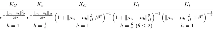
K :X×X → L(Y) as the reproducing kernel (we will present some concrete examples of K in Section 3; see Table 1);Kµx ∈L(Y,H) is defined as
K(µx, µt)(y) = (Kµty)(µx), (∀µx, µt∈X), orK(·, µt)(y) =Kµty. (3)
Further,f(µx) =Kµ∗xf (∀µx ∈X, f ∈H).
• Regression function: Let ρ be the µ-induced probability measure on the Z =X×Y
product space, and letρ(µx, y) =ρ(y|µx)ρX(µx) be the factorization ofρ into conditional and marginal distributions.7 The regression function ofρ with respect to the (µx, y) pair is denoted by
fρ(µa) = Z
Y
ydρ(y|µa) (µa∈X) (4)
and for f ∈ L2ρX let kfkρ = qhf, fiρ := kfkL2
ρX =
hR
Xkf(µa)k
2
Y dρX(µa) i12
. Let us
assume that the operator-valued kernel K :X×X → L(Y) is a Mercer kernel (that is
H =H(K) ⊆C(X, Y) ={X → Y continuous functions}), is bounded (∃BK <∞ such that kK(x, x)kL(Y) ≤BK), and is a compact operator for allx∈X. These requirements will be guaranteed by our assumptions, see Section 7.2.6. In this case, the inclusion SK∗:
H ,→L2
ρX is bounded, and its adjoint SK:L 2
ρX →H is given by
(SKg)(µu) = Z
X
K(µu, µt)g(µt)dρX(µt). (5)
We further define ˜T as
˜
T =SK∗SK :L2ρX →L 2
ρX; (6)
in other words, the result of operation (5) belongs to H, which is embedded inL2ρX. ˜T is a compact, positive, self-adjoint operator (Carmeli et al., 2010, Proposition 3), thus by the spectral theorem ˜Ts exists, wheres≥0.
6. Thex7→µxmapping is defined forallx∈M+1(X) ifkis bounded, i.e., supu∈Xk(u, u)<∞.
2.2 Distribution Regression
We now formally define the distribution regression task. Let us assume that M+1(X) is endowed with S1 = B(τw), the weak-topology generated σ-algebra; thus (M+1(X),S1) is
a measurable space. In the distribution regression problem, we are given samples ˆz =
{({xi,n}Nn=1i , yi)}li=1 with xi,1, . . . , xi,Ni
i.i.d.
∼ xi where z = {(xi, yi)}li=1 with xi ∈ M+1 (X) and yi ∈ Y drawn i.i.d. from a joint meta distribution M defined on the measurable space (M+1(X)×Y,S1 ⊗ B(Y)), the product space enriched with the product σ-algebra. Unlike in classical supervised learning problems, the problem at hand involves two levels of randomness, wherein first z is drawn from M, and then ˆz is generated by sampling points fromxifor alli= 1, . . . , l. The goal is to learn the relation between the random distribution
x and response y based on the observed ˆz. For notational simplicity, we will assume that
N =Ni (∀i).
As in the classical regression problem (Rd→R), distribution regression can be tackled
via kernel ridge regression (using a squared loss as the discrepancy criterion). The kernel (say KG) is defined on M+1(X), and the regressor is then modelled by an element in the RKHS G = G(KG) of functions mapping from M+1(X) to Y. In this paper, we choose
KG(x, x0) =K(µx, µx0) wherex, x0 ∈M+
1(X) and so that the function (inG) to describe the
(x, y) random relation is constructed as a compositionf ◦µx, i.e.
M+ 1 (X)
µ
−→X(⊆H =H(k))−−−−−−−→f∈H=H(K) Y. (7) In other words, the distribution x ∈ M+
1 (X) is first mapped to X ⊆ H by the mean
embedding µ, and the result is composed withf, an element of the RKHSH. Let the expected risk for a ˜f :X→Y (measurable) function be defined as
R˜
f=E(x,y)∼M
f˜(µx)−y
2
Y,
which is minimized by thefρ regression function. The classical regularization approach is to optimize
fzλ = arg min f∈H
1
l
l X
i=1
kf(µxi)−yik 2
Y +λkfk
2
H (8)
instead ofR, based on samplesz. Sincezis not available, we consider the objective function defined by the observable quantity ˆz,
fˆzλ = arg min f∈H
1
l
l X
i=1
kf(µxˆi)−yik 2
Y +λkfk
2
H, (9)
where ˆxi = N1 PNn=1δxi,n is the empirical distribution determined by{xi,n}
N
i=1. The ridge
regression objective function has an analytical solution: given training samples ˆz, the pre-diction for a new ttest distribution is
(fzˆλ◦µ)(t) =k(K+lλI)−1[y1;. . .;yl], (10)
where k = [K(µxˆ1, µt), . . . , K(µxˆl, µt)] ∈ L(Y)
1×l, K = [K(µ
ˆ
xi, µxˆj)] ∈ L(Y)
l×l,
Remark 1
• It is important to note that the algorithm has access to the sample points only via
their mean embeddings {µxˆi}
l
i=1 in Eq. (9).
• There is a two-stage sampling difficulty to tackle: The transition from fρ to fzλ
rep-resents the fact that we have only l distribution samples (z); the transition from fzλ
to fˆzλ means that the xi distributions can be accessed only via samples (ˆz).
• While ridge regression can be performed using the kernel KG, the two-stage sam-pling makes it difficult to work with arbitrary KG. By contrast, our choice of
KG(x, x0) = K(µx, µx0) enables us to handle the two-stage sampling by estimating
µx with an empirical estimator, and using it in the algorithm as shown above.
• In case of scalar output (Y = R), L(Y) = L(R) = R and (10) is a standard linear
equation with K∈Rl×l, k∈R1×l. More generally, if Y =Rd, then L(Y) =L(Rd) = Rd×d and (10) is still a finite-dimensional linear equation with K ∈ R(dl)×(dl) and k∈Rd×(dl).
• One could also formulate the problem (and get guarantees) for more abstract X ⊆
H→Y regression tasks [see Eq. (7)] on a convex set X with H and Y being general, separable Hilbert spaces. Since distribution regression is probably the most accessi-ble example where two-stage sampling appears, and in order to keep the presentation simple, we do not consider such extended formulations in this work.
Our main goals in this paper are as follows: first, to analyse the excess risk
E fˆzλ, fρ
:=R[fˆzλ]− R[fρ],
both whenfρ∈H(the well-specified case) andfρ∈L2ρX\H(the misspecified case); second,
to establish consistency (E fˆzλ, fρ
→ 0, or in the misspecified case E fˆzλ, fρ
−D2H → 0, whereD2
H:= infq∈Hkfρ−S∗Kqk
2
ρis the approximation error offρ by a function inH); and third, to derive an exact computational-statistical efficiency trade-off as a function of the (l, N, λ) triplet, and of the difficulty of the problem.
3. Assumptions
In this section, we detail our assumptions on the (X, Y, k, K) quartet. Our analysis for the well-specified case uses existing ridge regression results (Caponnetto and De Vito, 2007) focusing on problem (8) where only a single-stage sampling is present, hence we have to verify the associated conditions. Though we make use of these results, the analysis still remains challenging; the available bounds can moderately shorten our proof. We must take particular care in verifying that Caponnetto and De Vito (2007)’s conditions are met, since they need to hold for the space of mean embeddings of the distributions (X=µ M+1(X)
), whose properties as a function of Xand H must themselves be established.
Our assumptions are as follows:
2. Y is a separable Hilbert space.
3. kis bounded, in other words∃Bk<∞such that supu∈Xk(u, u)≤Bk, and continuous. 4. The {Kµa}µa∈X operator family is uniformly bounded in Hilbert-Schmidt norm and
H¨older continuous in operator norm. Formally,∃BK <∞ such that
kKµak 2
L2(Y,H) =T r K
∗ µaKµa
≤BK, (∀µa∈X), (11)
and∃L >0,h∈(0,1] such that the mappingK(·):X→L(Y,H) is H¨older continuous: kKµa−KµbkL(Y,H) ≤Lkµa−µbk
h
H, ∀(µa, µb)∈X×X. (12)
5. y is bounded: ∃C <∞ such that kykY ≤C almost surely.
These requirements hold under mild conditions: in Section 8, we provide insight into the consequences of our assumptions, with several concrete illustrations (e.g. regression with set- and RBF-type kernels).
4. Error Bounds, Consistency & Computational-Statistical Efficiency Trade-off
In this section, we present our analysis of the consistency of the mean embedding based ridge regression (MERR) method.
Given the estimator (fˆzλ) in Eq. (9), we derive finite-sample high probability upper bounds (see Theorems 2 and 7) for the excess riskE fˆzλ, fρ
, and in the misspecified setting, for the excess risk compared to the best attainable value fromH, i.e.,E fˆzλ, fρ
−DH2. We illustrate the bounds for particular classes of prior distributions, and work through special cases to obtain consistency conditions and computational-statistical efficiency trade-offs (see Theorems 4, 9 and the 3rd bullet of Remark 8). The main challenge is how to turn the convergence rates of the mean embeddings into those for an error E of the predictor. Although the main ideas of the proofs can be summarized relatively briefly, the full details are more demanding. High-level ideas with the sketches of the proofs and the obtained results are presented in Section 4.1 (well-specified case) and Section 4.2 (misspecified case). The derivations of some technical details of Theorems 2 and 7 are available in Section 7.
4.1 Results for the Well-specified Case
We first focus on the well-specified case (fρ ∈ H) and present our first main result. We derive a high probability upper bound for the excess risk E fˆzλ, fρ
of the MERR method (Theorem 2). The upper bound is instantiated for a general class of prior distributions (Theorem 4), which leads to a simple computational-statistical efficiency description (The-orem 5); this shows (among others) conditions when the MERR technique is able to achieve theone-stage sampled minimax optimal rate. We first give a high-level sketch of our con-vergence analysis and an intuitive interpretation of the results. An outline of the main proof ideas is given below, with technical details in Section 7.
Let us definex={xi}li=1and ˆx={{xi,n}Nn=1}li=1as the ‘x-part’ ofzand ˆz, respectively.
as
fzλ= (Tx+λ)−1gz, Tx= 1
l
l X
i=1
Tµxi, gz=
1
l
l X
i=1
Kµxiyi, (13)
fˆzλ= (Txˆ +λ)−1gˆz, Tˆx=
1
l
l X
i=1
Tµxiˆ , gˆz=
1
l
l X
i=1
Kµxiˆ yi, (14)
whereTµa =KµaK
∗
µa ∈L(H) (µa∈X),Tx, Txˆ :H→H,gz, gˆz∈H. By these explicit
ex-pressions, one can decompose the excess risk into 5 terms (Szab´o et al., 2015, Section A.1.8):
E fˆzλ, fρ
=R fˆzλ
− R[fρ]≤5 [S−1+S0+A(λ) +S1+S2],
where
S−1 =S−1(λ,z,ˆz) =k √
T(Txˆ+λI)−1(gˆz−gz)k2H, (15) S0 =S0(λ,z,ˆz) =k
√
T(Txˆ +λI)−1(Tx−Txˆ)fzλk2H, (16)
A(λ) =k√T(fλ−fρ)k2H, S1 =S1(λ,z) =k √
T(Tx+λI)−1(gz−Txfρ)k2H,
S2 =S2(λ,z) =k √
T(Tx+λI)−1(T−Tx)(fλ−fρ)k2H,
fλ = arg min f∈H
(R[f] +λkfk2H), T = Z
X
TµadρX(µa) =SKS
∗
K :H→H. (17)
Three of the terms (S1, S2, A(λ)) are identical to the terms in Caponnetto and De Vito
(2007), hence the earlier bounds can be applied. The two new terms (S−1, S0) resulting
from two-stage sampling will be upper bounded by making use of the convergence of the empirical mean embeddings. These bounds will lead to the following results:
Theorem 2 (Finite-sample excess risk bounds; well-specified case) Let
K(·) : X → L(Y,H) be H¨older continuous with constants L, h. Let l ∈ Z+, N ∈ Z+,
0< λ, 0 < η <1, 0 < δ, Cη = 32 log2(6/η), kykY ≤C (a.s.) and A(λ) be the residual as
defined above. Define M = 2(C+kfρkH
√
BK), Σ = M2 , T as in (17), B(λ) =kfλ−fρk2H
as the reconstruction error, andN(λ) =T r[(T+λI)−1T]as the effective dimension. Then with probability at least 1−η−e−δ, the excess risk can be upper bounded as
Efˆzλ, fρ
≤5
(4L21 +plog(l) +δ2h(2B k)h
λNh
C2+ 4BK×
× log2 6 η 64 λ
M2B
K
l2λ +
Σ2N(λ)
l
+24
λ2
4BK2B(λ)
l2 +
BKA(λ)
l
+B(λ) +kfρk2H
+A(λ) +Cη
B2
KB(λ)
l2λ +
BKA(λ) 4lλ +
BKM2
l2λ +
Σ2N(λ)
l
)
if l≥2CηBKN(λ)/λ, λ≤ kTkL(H) and N ≥ 1 +
p
log(l) +δ22h+6h Bk(BK)
Below we specialize our excess risk bound for a general prior class, which captures the diffi-culty of the regression problem as defined in Caponnetto and De Vito (2007). ThisP(b, c) class is described by two parametersband c: largerbmeans faster decay of the eigenvalues of the covariance operator T [in Eq. (17)], hence smaller effective input dimension; largerc
corresponds to a smoother regression function. Formally:
Definition of the P(b, c) class: Let us fix the positive constants R, α, β. Then given 1 < b, c ∈ (1,2], the P(b, c) class is the set of probability distributions ρ on Z = X×Y
such that
1. a range space assumption is satisfied: ∃g∈H s.t.fρ=T
c−1
2 gwith kgk2
H≤R, 2. in the spectral decomposition of T =P∞
n=1λnh·, eniHen, where (en)
∞
n=1 is a basis of
Ker(T)⊥, the eigenvalues ofT satisfyα ≤nbλn≤β (∀n≥1).
Remark 3 We make few remarks about the P(b, c) class:
• Range space assumption on fρ: The smoothness of fρ is expressed as a range space
assumption, which is slightly different from the standard smoothness conditions ap-pearing in non-parametric function estimation. By the spectral decomposition of T
given above [λ1 ≥λ2≥. . . >0,limn→∞λn = 0], Tru=P∞n=1(λn)rhu, eniHen (r= c−1
2 ≥0, u∈H) and
Im(Tr) =n X∞
n=1cnen:
X∞
n=1c 2
nλ −2r n <∞
o
. (18)
Specifically, in the limit as r → 0, we obtain fρ ∈ Im(T0) = Im(I) = H (no
con-straint); larger values of r give rise to faster decay of the(cn)∞n=1 Fourier coefficients. This is the concrete meaning of fρ∈Im(Tr).
• Spectral decay condition: We can provide a simple illustration of when the spectral decay conditions hold, in the event that the distributions are normal with means mi
and identical variance (xi =N(mi, σ2I)). When Gaussian kernels (k) are used with
linear K, then K(µxi, µxj) = e
−ckmi−mjk2 (Muandet et al., 2012, Table 1, line 2)
(Gaussian, with arguments equal to the difference in means). Thus, this Gram matrix will correspond to the Gram matrix using a Gaussian kernel between points mi. The
spectral decay of the Gram matrix will correspond to that of the Gaussian kernel, with points drawn from the meta-distribution over themi. Thus, the source conditions are
analysed in the same manner as for Gaussian Gram matrices: see e.g. Steinwart and Christmann (2008) for a discussion of these spectral decay properties.
In theP(b, c) family, the behaviour ofA(λ),B(λ) andN(λ) is known: A(λ)≤Rλc,B(λ)≤
Rλc−1,N(λ)≤βb−b1λ−1b. Specializing Theorem 2 and retaining its assumptions, we get: Theorem 4 (Finite-sample excess risk bound for ρ∈ P(b, c))
Then
Efˆzλ, fρ
≤5 (
4L2
1 +plog(l) +δ 2h
(2Bk)h
λNh
"
C2+ 4BK×
× Cη (
2
λ "
M2BK
l2λ +
Σ2βb
(b−1)lλ1b
# + 3
4λ2
4BK2Rλc−1
l2 +
BKRλc
l
)
+Rλc−1+kfρk2H !#
+Rλc+Cη "
BK2 Rλc−2
l2 +
BKRλc−1 4l +
BKM2
l2λ +
Σ2βb
(b−1)lλ1b
# ) .
Discarding the constants in Theorem 4, the study of convergence of the excess riskE(fλ
ˆ
z, fρ)
to 0 boils down to findingN and λ(as a function of l) whereN → ∞,λ→0 and
r(l, N, λ) = log h(l)
Nhλ
1
λ2l2 + 1 +
1
lλ1+1b
+λc+ 1
l2λ+
1
lλ1b
→0, s.t. lλb+1b ≥1,log(l)
λ2h ≤N
(19)
asl→ ∞. Let us chooseN =lahlog(l); in this case Eq. (19) reduces to
r(l, λ) = 1
l2+aλ3 +
1
laλ+ 1
la+1λ2+1b +λ
c+ 1
l2λ+
1
lλ1b
→0, s.t. lλb+1b ≥1, laλ2≥1. (20)
One can assume that a >0, otherwise r(l, λ) → 0 fails to hold; in other words, N should grow faster than log(l). Matching the ‘bias’ (λs) and ‘variance’ (other) terms in r(l, λ) to choose λ, and guaranteeing that the matched terms dominate and the constraints in Eq. (20) hold, one gets the following simple description for the computational-statistical efficiency trade-off:8
Theorem 5 (Computational-statistical efficiency trade-off; well-specified case;
ρ ∈ P(b, c)) Suppose the conditions in Theorem 2 hold. Let ρ∈ P(b, c) and N =lahlog(l), where 0< a, 1< b, c∈(1,2]. If
• a≤ bbc(c+1+1), then E fˆzλ, fρ
=Opl−cac+1
with λ=l−c+1a ,
• a≥ bbc(c+1+1) thenE fˆzλ, fρ
=Opl−bcbc+1
withλ=l−bcb+1.
Remark 6 Theorem 5 formulates an exact computational-statistical efficiency trade-off for the choice of the bag size (N) as a function of the number of distributions (l) and problem difficulty (b, c).
• a-dependence: A smaller bag size (smaller a; N = lhalog(l)) means computational savings, but reduced statistical efficiency. It is not worth increasing a above bbc(c+1)+1 since from that point the rate becomesr(l) =l−bcbc+1; remarkably, this rate is minimax
in the one-stage sampled setup (Caponnetto and De Vito, 2007). The sensible choice
a= bbc(c+1)+1 <2 means that the one-stage sampled minimax rate can be achieved in the two-stage sampled setting with bag size N sub-quadratic in l.
• h-dependence: In accord with our ‘smoothness’ assumptions it is rewarding to use smoother K kernels (largerh∈(0,1]) since this reduces the bag size [N =lahlog(l)].
• c-dependence: The strictly decreasing property of c 7→ b(bcc+1)+1 implies that for ‘smoother’ problems (larger c) fewer samples (N) are sufficient.
Below we elaborate on the sketched high-level idea and prove Theorem 2.
Proof of Theorem 2(detailed derivations of each step can be found in Section 7.1)
1. Decomposition of the excess risk: We have the following upper bound for the excess risk
E fˆzλ, fρ
=R fzˆλ
− R[fρ]≤5 [S−1+S0+A(λ) +S1+S2]. (21)
2. It is sufficient to upper bound S−1 and S0: Caponnetto and De Vito (2007) have
shown that for ∀η > 0 if l ≥ 2CηBKN(λ)/λ, λ ≤ kTkL(H), then P(Θ(λ,z) ≤ 1/2) ≥
1−η/3, where
Θ(λ,z) =(T −Tx)(T+λI)−1
L(H), (22)
using which upper bounds on S1 and S2 that hold with probability 1−η are obtained.
It is known thatA(λ)≤Rλc.
3. Probabilistic bounds on kgˆz−gzk2H, kTx−Tˆxk2L(H), k √
T(Tˆx+λI)−1kL2(H), kfzλk2H:
One can boundS−1 and S0 as
S−1 ≤
√
T(Tˆx+λI)−1
2
L(H)kgˆz−gzk 2
H
and
S0 ≤
√
T(Tˆx+λI)−1
2
L(H)kTx−Txˆk 2
L(H)
fzλ
2
H.
For the terms on the r.h.s., we derive upper bounds [for the definition ofα, see Eq. (24)]
kgˆz−gzk2H≤L2C2
(1 +√α)2h(2Bk)h
Nh ,
√
T(Txˆ+λI)−1
L(H) ≤ √2
λ,
kTx−Txˆk2L(H)≤
(1 +√α)2h2h+2(Bk)hBKL2
Nh ,
and
f
λ
z
2
H≤6
16
λ log
2
6
η
M2B
K
l2λ +
Σ2N(λ)
l
(23)
+ 4
λ2 log 2
6
η
4BK2B(λ)
l2 +
BKA(λ)
l
+B(λ) +kfρk2H
.
• kgˆz−gzk2H (see Section 7.1.1): if the empirical mean embeddings are close to their
population counterparts, i.e.,
kµxi−µxˆikH ≤
(1 +√√α)√2Bk
N , (∀i= 1, . . . , l). (24)
This event has probability 1−le−α over all i = 1, . . . , l samples; see (Altun and Smola, 2006) and (Szab´o et al., 2015, Section A.1.10).
• kTx−Tˆxk2L(H) (see Section 7.1.2): (24) is assumed.
• k√T(Txˆ +λI)−1kL2(H) (Szab´o et al., 2015, Section A.1.11): (24),Θ(λ,z)≤ 12, and
(1 +√α)22h+6h Bk(BK)
1
hL
2
h
λh2
≤N. (25)
• kfzλk2
H: The bound is guaranteed to hold under the conditions of the bounds ofS1
and S2.8
4. Union bound: By applying an α = log(l) +δ reparameterization, and combining the received upper bounds with Caponnetto and De Vito (2007)’s results for S1 and S2,
Theorem 2 follows (Section 7.1.3) with a union bound.
Finally, we note that existing results/ideas were used at two points to simplify our anal-ysis: boundingS1,S2, Θ(λ,z),
fzλ
2
H (Caponnetto and De Vito, 2007) and kµxi−µxˆikH (Altun and Smola, 2006).9
4.2 Results for the Misspecified Case
In this section, we focus on the misspecified case (fρ∈L2ρX\H) and present our second main
result, which was inspired by the proof technique of Sriperumbudur et al. (2014, Theorem 12). We derive a high probability upper bound for E fˆzλ, fρ
, i.e., the excess risk of the MERR method (Theorem 7) which gives rise to consistency results (3rd bullet of Remark 8) and precise computational-statistical efficiency trade-off (Theorem 9). Theorem 7 consists of two finite-sample bounds:
1. The first, more general bound [Eq. (27)] will be used to show consistency in the misspecified case (see the 3rd bullet of Remark 8), in other words thatE fˆzλ, fρ
can be driven to its smallest possible value determined by the “richness” of H:
DH2 := inf
q∈Hkfρ−S ∗ Kqk
2
ρ. (26)
The value ofDHequals the approximation error offρ by a function fromH. Specifi-cally, if H [preciselySK∗ (H) ={SK∗q :q∈H} ⊆L2ρX] is dense inL2ρX, thenDH= 0.
2. The second, specialized result [Eq. (28)] under additional smoothness assumptions on
fρ will give rise to a precise computational-statistical efficiency trade-off in terms of the problem difficulty (s) and sample numbers (l, N); this result can be seen as the misspecified analogue of Theorem 5.
After stating our results, the main ideas of the proof follow; further technical details are available in Section 7.2. Our main theorem for bounding the excess risk is as follows:
Theorem 7 (Finite-sample excess risk bounds; misspecified case) Let l ∈ Z+,
N ∈ Z+, 0 < λ, 0 < η < 1, 0 < δ and C
η = log
6
η
. Assume that
12BK
λ Cη 2
≤ l
and 1 +plog(l) +δ22h+6h Bk(BK)
1
hL
2
h/λ
2
h ≤N.
1. Then for arbitrary q ∈H with probability at least 1−η−e−δ
q
E fˆzλ, fρ
≤
2LC1 +plog(l) +δh(2Bk)
h
2
√
λNh2
1 +2
√ BK √ λ + (27)
2√Cη
λ (
2C√BK
l +
C√√BK
l !
+
2BK
l + σ √ l 1 λ q
λkfρkρDa(λ, q) )
+Da(λ, q),
where Da(λ, q) =kfρ−SK∗qkρ+ max(1,kTkL(H))λ
1 2kqkH.
2. In addition, suppose fρ∈Im( ˜Ts)for somes >0, whereT˜is defined in Eq.(6). Then
with probability at least 1−η−e−δ, we have
q
E fλ
ˆ
z, fρ
≤
2LC1 +plog(l) +δh(2Bk)
h
2
√
λNh2
1 +2
√ BK √ λ +
2√Cη
λ (
2C√BK
l +
C√√BK
l !
+
2BK
l + σ √ l 1 λ× s max 1, T˜ s
L(L2
ρX) λ T˜
−sf ρ
ρDb(λ, s) )
+Db(λ, s), (28)
where Db(λ, s) = max(1,kT˜ksL−(L12
ρX))λ
min(1,s)kT˜−sf ρkρ.
Remark 8 We give a short insight into the assumptions of Theorem 7, followed by conse-quences of the theorem.
• Range space assumption on fρ: The range space assumption for the compact, posi-tive, self-adjoint operator, T˜ = ˜T(K) : L2ρX → L2ρX in the 2nd part of Theorem 7 can be interpreted similarly to that on T; see Eq. (18). One can also prove alterna-tive descriptions for Im( ˜Ts) in terms of interpolation spaces (Steinwart and Scovel, 2012, Theorem 4.6, page 387), or the decay of the 2-approximation error function,
A2(λ) = inff∈H(K)
λkfk2H(K)+R[f]− R[fρ]
• qE fλ
ˆ
z, fρ
: Notice that in the bounds [(27),(28)], instead of the excess risk, its square root appears; this has technical reasons, as it is easier to have the Da(λ, q) quantity (without multiplicative constants) appear on the r.h.s. of Eq. (27) with this form.
• Consistency in the misspecified case: The consequence of Theorem 7(1) is as follows. Discarding the constants in Eq. (27), we obtain the upper bound (notice that the constant multiplier of kfρ−SK∗qkρ in the last term was one):
p
r(l, N, λ, q) = log
h
2(l)
Nh2λ
+√1
lλ+
q
fρ−SK∗q
ρ+
√
λkqkH
λ√l +kfρ−S
∗ Kqkρ+
√
λkqkH.
By choosing N =l1/hlogl, pr(l, λ) is bounded by
inf q∈H
kfρ−SK∗ qkρ+ q
fρ−SK∗ q ρ
λ√l +
p
kqkH
λ34
√
l +
√
λkqkH
+Op
1 √ λl .
Our goal is to investigate the behavior of the bound as l → ∞, λ → 0 and λ√l → ∞. Define K(α, β, γ) := infq∈H
n
kfρ−SK∗qkρ+α q
fρ−SK∗q
ρ+β p
kqkH+γkqkH
o
.
K(α, β, γ) is the pointwise infimum of affine functions, therefore it is upper semi-continuous and concave on R3 (Aliprantis and Border, 2006, Lemmas 2.41 and 5.40
); it is continuous on ×3
i=1R>0 (Rockafellar and Wets, 2008, Theorem 2.35). More-over, by applying (Rockafellar and Wets, 2008, Corollary 2.37) it extends continuously to ×3
i=1R≥0; specifically it is continuous at (α, β, γ) =0. In other words, as l→ ∞, λ→0 and λ√l → ∞, K
1
λ√l,
1
λ34
√ l,
√
λ
→ DH and we get consistency in the misspecified
case,10
p
r(N, l, λ)→DH.
Discarding the constants in Eq. (28) we get10 p
r(l, N, λ) = log
h
2(l)
Nh2λ
+√1
lλ+
√
λmin(1,s)
λ√l +λ
min(1,s), subject to 1
λ2 ≤l. (29)
Our goal is to drive r(l, N, λ) to zero with a suitable choice of the (l, N, λ) triplet under the stronger range space assumption. Since in Eq. (29) min(1, s) appears, one can assume without loss of generality that s∈(0,1]; consequently 1− s2 ∈1
2,1
and 1 l12λ12
≤ 1
λ1−s2l12.
Let us choose N = l2a/hlog(l); in this case using the previous dominance note, Eq. (29) reduces to the study of
p
r(l, λ) = 1
laλ+ 1
λ1−s2l 1 2
+λs→0, s.t. lλ2≥1. (30) One can assume that a >0, otherwise r(l, λ) → 0 fails to hold: in other words, N should grow faster than log(l). Matching the ‘bias’ (λs) and ‘variance’ (other) terms in r(l, λ) to choose λ, guaranteeing that the matched terms dominate and the constraint in Eq. (30) hold, one can arrive at the following computational-statistical efficiency trade-off:8
Theorem 9 (Computational-statistical efficiency trade-off; misspecified case,
fρ ∈ Im( ˜Ts)) Suppose that fρ ∈ Im( ˜Ts) and N = l
2a
h log(l), where s ∈ (0,1], a > 0. If
• a≤ ss+1+2, then E fˆzλ, fρ
=Op
l−s2+1sa
withλ=l−s+1a ,
• a≥ ss+1+2, then E fλ
ˆ
z, fρ
=Op
l−s2+2s
withλ=l−s+21 .
Remark 10 Theorem 9 provides a complete computational-statistical efficiency trade-off description for the choice of the bag size (N) as a number of the distributions (l).
• a-dependence: A smaller value of ‘a’ (smaller bagsN =l2a/hlog(l)) leads to a compu-tational advantage, but one looses in statistical efficiency. As ‘a’ reaches ss+1+2, the rate becomesr(l) =l−s2+2s and one does not gain from further increasing the value of a. The
sensible choice of a= ss+1+2 ≤ 2
3 means thatN can again be sub-quadratic(2a < 4 3 <2) in l.
• h-dependence: By using smoother K kernels (larger h∈(0,1]) one can reduce the size of the bags: h 7→ 2a/h is decreasing in h. This is compatible with our smoothness requirement on fρ.
• s-dependence: “Easier” tasks (largers) give rise to faster convergence. Indeed, in the
r(l) =l−s2+2s rate the s7→ 2s
s+2 exponent is strictly increasing function of the problem difficulty (s). For example, for extremely non-smooth regression problems (s ≈ 0) the convergence can be arbitrary slow (lims→0 s2+2s = 0). In the smooth case (s = 1)
lims→1s2+2s = 23 and one can achieve the r(l) =l−
2 3 rate.
• We may compare our r(l) =l−s2+2s result with the r
o(l) =l−
2s
2s+1 (one-stage sampled)
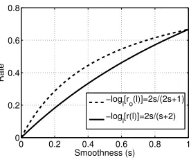
rate (Steinwart et al., 2009, β/2 := s, q := 2, p := 1 in Corollary 6), which was shown to be asymptotically optimal on Y = R for continuous k on compact metric X. Steinwart et al.’s result is more general in terms of q (kfkqH based regularization) and p (kfk∞ ≤ CkfkpHkfk1ρ−p, ∀f ∈ H; in our case p = 1), although it imposes an additional eigenvalue constraint [(Steinwart et al., 2009, Eq. (6))] as well as fρ∈
Im( ˜Ts). Moreover, one can observe that ro(l) ≤ r(l) with a small gap, and that for s→ 0 and s= 1, ro(l) = r(l); see Fig. 1. We further remind the reader that our
MERR analysis also holds for separable Hilbertoutput spacesY,separable topological
domains X enriched with a bounded, continuous kernelk, and that we handle the two-stage sampled setting.
The main steps of the proof of Theorem 7 are as follows:
Proof of Theorem 7(the details of the derivation are available in Section 7.2) Steps 1-7 will be identical in both proofs,11 and we present them jointly.
1. Decomposition of the excess risk: By the triangle inequality, we have q
E fzˆλ, fρ
=SK∗ fˆzλ−fρ
ρ≤
SK∗ fˆzλ−fzλ
ρ+
SK∗fzλ−fρ
ρ. (31)
0 0.2 0.4 0.6 0.8 1 0 0.2 0.4 0.6 0.8 Smoothness (s) Rate −log
l[ro(l)]=2s/(2s+1) −logl[r(l)]=2s/(s+2)
Figure 1: Comparison of thero(l) =l−
2s
2s+1 andr(l) =l− 2s
s+2 rates as function of the problem
difficulty/smoothness (s).
2. Bound on SK∗ fˆzλ−fzλ
ρ: Using
12 the fact that kSK∗ hk2ρ=
√
T h
2
H (∀h∈H), (32)
and the definitions of S−1 and S0 [see Eqs. (15)-(16)], we obtain
SK∗ fˆzλ−fzλ ρ= √
T fˆzλ−fzλ H≤
p S−1+
p
S0, (33)
through an application of triangle inequality. One can derive without a P(b, c) prior assumption (Section 7.2.1) the upper bound13
p S−1+
p S0 ≤
2LC(1 +√α)h(2Bk)
h
2
√
λNh2
1 +2
√
BK
√
λ
for the r.h.s. of Eq. (33) under the conditions that Θ(λ,z) ≤ 1
2 (which holds with
probability 1−η if [12BKlog(2/η)/λ]2≤l), and that Eqs. (24)-(25) hold. 3. Decomposition of SK∗fzλ−fρ
ρ: By the triangle inequality and Eq. (32), we have
SK∗ fzλ−fρ
ρ=
SK∗ fzλ−fλ
+SK∗ fλ−fρ
ρ≤
SK∗ fzλ−fλ
ρ+
SK∗fλ−fρ ρ
=
√
T fzλ−fλ H+
SK∗fλ−fρ
ρ. (34)
4. Decomposition of
√
T fzλ−fλ H: Making use of the analytical expressions forfzλ andfλ[see Eq. (13) and Eq. (17)], and the operator Woodbury formula (Ding and Zhou, 2008, Theorem 2.1, page 724) we arrive at the decomposition (see Section 7.2.2)
√
T fzλ−fλ H≤
√
T(Tx+λI)−1 L(H)
kgz−gρkH+
kT−TxkL(H)λ−1SK
fρ−( ˜T+λI)−1SK∗SKfρ
H
,
wheregρ=SKfρ. As it is known (Caponnetto and De Vito, 2007, page 348)k
√
T(Tx+ λI)−1kL(H)≤1/√λprovided that Θ(λ,z)≤ 12.
12. See for example de Vito et al. (2006) on page 88 with the (H,G, A, T) := (H, L2ρX, S ∗
5. Bound on kgz−gρkH, kT −TxkL(H): By concentration arguments the bounds
kgz−gρkH≤
4C√BK
l +
2C√BK
√ l ! log 2 η
, kT−TxkL(H)≤
4BK
l + 4σ √ l log 2 η
hold with probability at least 1−η, each (see Section 7.2.3, 7.2.4).
6. Decomposition of SK
fρ−( ˜T+λI)−1SK∗ SKfρ
2
H: Exploiting the analytical formula forfλ, one can construct (Section 7.2.5) the upper bound
SK
fρ−( ˜T+λI)−1SK∗SKfρ 2 H≤ T˜
fρ−( ˜T +λI)−1SK∗SKfρ
ρ
SK∗fλ−fρ ρ.
7. Bound on T˜
fρ−( ˜T +λI)−1SK∗SKfρ
ρ: Using our assumptions thatfρ ∈ Im( ˜T s)
(s ≥ 0)14 and exploiting the separability of L2ρX, by Lemma 7.3.2 (K = L2ρX, f = fρ,
M = ˜T,a= 1) and ˜T =SK∗SK we obtain the upper bound
T˜
fρ−( ˜T +λI)−1SK∗ SKfρ
ρ=
T˜
fρ−( ˜T+λI)−1T f˜ ρ
ρ
≤max1,kT˜ks L(L2
ρX)
λmin(1,s+1) T˜−sfρ
ρ= max
1,kT˜ks L(L2
ρX)
λT˜−sfρ
ρ,
where we used at the last step that min(1, s+ 1) = 1; this follows from s≥0.
8. Bound on SK∗fλ−fρ ρ:
(a) No range space assumption: One can construct (Section 7.2.6) the bound
SK∗fλ−fρ
ρ≤ kfρ−S ∗
Kqkρ+ max 1,kTkL(H)
λ12 kqk
H,
which holds for arbitraryq ∈H. (b) Range space assumption in L2
ρX: Using the S
∗
Kfλ = ( ˜T +λI)−1T f˜ ρ identity [see Eq. (43)], and Lemma 7.3.2 (M = ˜T,K=L2
ρX,a= 0), we get
SK∗fλ−fρ
ρ=
( ˜T+λI)−1T f˜ ρ−fρ
ρ≤max
1,T˜
s−1
L(L2
ρX)
λmin(1,s)T˜−sfρ
ρ.
9. Union bound: Applying an α = log(l) +δ reparameterization, changing η to η3 and combining the derived results (in case of the first statement with s= 0) with a union bound, Theorem 7 follows.
Remark 11 To contrast the derivation of the well- and the misspecified cases, we note that previous results [Section 4.1, or Caponnetto and De Vito (2007)’s bound] were used at two points:
(a) In Step 2 by using Eq. (32) and transforming the L2ρ
X error
SK∗ fˆzλ−fzλ
ρ to H,
we could rely on our previous bounds for S−1 and S0. However, we were required to use a different concentration argument to guarantee Θ(λ,z) ≤ 1
2 since we no longer assume theP(b, c) prior class.
(b) In Step 4 the first term could be bounded by Caponnetto and De Vito (2007). Its Θ(λ,z)≤ 12 condition was guaranteed by Step 2; and see Section 7.2.1.
We note that our misspecified proof method was inspired by Sriperumbudur et al. (2014, Theorem 12), where the authors focused on the consistency of an infinite-dimensional ex-ponential family estimator.
5. Related Work
In this section we discuss existing approaches and heuristic techniques to tackle learning problems on distributions.
Methods based on parametric assumptions: A number of methods have been proposed to compute the similarity of distributions or bags of samples. As a first approach, one could fit a parametric model to the bags, and estimate the similarity of the bags based on the obtained parameters. It is then possible to define learning algorithms on the basis of these similarities, which often take analytical form. Typical examples with explicit formulas include Gaussians, finite mixtures of Gaussians, and distributions from the exponential family (with known log-normalizer function and zero carrier measure, see Kondor and Jebara, 2003; Jebara et al., 2004; Wang et al., 2009; Nielsen and Nock, 2012). A major limitation of these methods, however, is that they apply quite simple parametric assumptions, which may not be sufficient or verifiable in practise.
Methods based on parametric assumption in a RKHS: A heuristic related to the parametric approach is to assume that the training distributions are Gaussians in a reproducing kernel Hilbert space (see for example Jebara et al., 2004; Zhou and Chellappa, 2006, and references therein). This assumption is algorithmically appealing, as many diver-gence measures for Gaussians can be computed in closed form using only inner products, making them straightforward to kernelize. A fundamental shortfall of kernelized Gaussian divergences is the lack of their consistency analysis in specific learning algorithms.
Kernels based techniques: A more theoretically grounded approach to learning on distributions has been to define positive definite kernels on the basis of statistical diver-gence measures on distributions, or by metrics on non-negative numbers; these can then be used in kernel algorithms. This category includes work on semigroup kernels (Cuturi et al., 2005), non-extensive information theoretical kernel constructions (Martins et al., 2009), and kernels based on Hilbertian metrics (Hein and Bousquet, 2005). For example, the intuition of semigroup kernels (Cuturi et al., 2005) is as follows: if two measures or sets of points overlap, then their sum is expected to be more concentrated. The value of dispersion can be measured by entropy or inverse generalized variance. In the second type of approach (Hein and Bousquet, 2005), homogeneous Hilbert metrics on the non-negative real line are used to define the similarity of probability distributions. While these techniques guaran-tee to provide valid kernels on certain restricted domains of measures, the performance of learning algorithms based on finite-sample estimates of these kernels remains a challenging open question. One might also plug into learning algorithms (based on similarities of dis-tributions) consistent R´enyi and Tsallis divergence estimates (P´oczos et al., 2011, 2012), but these similarity indices are not kernels, and their consistency in specificlearning tasks
Multi-instance learning: An alternative paradigm in learning when the inputs are “bags of objects” is to simply treat each input as afinite set: this leads to the multi-instance learning task (MIL, see Dietterich et al., 1997; Ray and Page, 2001; Dooly et al., 2002). In MIL one is given a set of labelled bags, and the task of the learner is to find the mapping from the bags to the labels. Many important examples fit into the MIL framework: for example, different configurations of a given molecule can be handled as a bag of shapes, images can be considered as a set of patches or regions of interest, a video can be seen as a collection of images, a document might be described as a bag of words or paragraphs, a web page can be identified by its links, a group of people on a social network can be captured by their friendship graphs, in a biological experiment a subject can be identified by his/her time series trials, or a customer might be characterized by his/her shopping records. The MIL approach has been applied in several domains; see the reviews from Babenko (2004); Zhou (2004); Foulds and Frank (2010); Amores (2013).
“Bag-of-objects” methods (MIL, classification): Despite the large number of MIL applications and the spate of heuristic solution techniques, there exist few theoretical results in the area (Auer, 1998; Long and Tan, 1998; Blum and Kalai, 1998; Babenko et al., 2011; Zhang et al., 2013; Sabato and Tishby, 2012) and they focus on the multi-instance
classification (MIC) task. In particular, let us first consider the standard MIC assumption (Dietterich et al., 1997), where a bag is declared to be positive (labelled with “1”) if at least one of its instances is positive (“1”); otherwise, the bag is negative (“0”).15 In other words, if the instances (xi,n) in theithbag {xi,1, . . . , xi,N}have hidden labelL(xi,n)∈ {0,1}, then the observed label of the bag is yi =h(xi,1, . . . , xi,N) = max(L(xi,1), . . . , L(xi,N))∈ {0,1}. In case of the original APR (axis-aligned rectangles; Dietterich et al., 1997) hypothesis class, functionLis equal to the indicator of an unknown rectangleR(L=IR). In other words, a bag is declared to be positive if there exists at least one instance in the bag, which belongs to R.16 The goal is to learn R with high probability given the bags ({xi,1, . . . , xi,N} -s) and their labels (yi-s). Long and Tan (1998) proved the PAC learnability (probably approximately correct; Valiant, 1984) of the APR hypothesis class, if all instances in each bag are i.i.d. and follow the same product distribution over the instance coordinates. On the other hand, for arbitrary distributions over bags, when the instances within a bag might be statistically dependent, APR learning under MIC is NP-hard (Auer, 1998); the same authors also showed that the product property (Long and Tan, 1998) on the coordinates is not required to obtain PAC results. Blum and Kalai (1998) extended PAC learnability of APR-s to hypothesis classes learnable from one-sided classification noise. In contrast to the previous approaches (Long and Tan, 1998; Auer, 1998; Blum and Kalai, 1998), Babenko et al. (2011) modelled the bags as low-dimensional manifolds, and proved PAC bounds. By relaxing the standard MIC assumption, Sabato and Tishby (2012) showed PAC-learnability for general MIC hypothesis classes with extended “max” functions. Zhang et al. (2013) derived high-probability generalization bounds in the MIC setting, when local and global representations are combined. Our work falls outside this setting since the label and bag generation mechanisms we consider are different: we do not assume an exact form of the
15. The motivation of this assumption comes from drug discovery: if a molecule has at least one well-binding configuration, then it is considered to bind well.