AD
3: Alternating Directions Dual Decomposition
for MAP Inference in Graphical Models
∗Andr´e F. T. Martins [email protected]
Priberam Labs,
Alameda D. Afonso Henriques 41, 2.◦, 1000–123 Lisboa, Portugal and
Instituto de Telecomunica¸c˜oes,
Av. Rovisco Pais 1, 1049–001 Lisboa, Portugal
M´ario A. T. Figueiredo [email protected]
Instituto de Telecomunica¸c˜oes, and Instituto Superior T´ecnico, Universidade de Lisboa Av. Rovisco Pais 1, 1049–001 Lisboa, Portugal
Pedro M. Q. Aguiar [email protected]
Instituto de Sistemas e Rob´otica, and Instituto Superior T´ecnico, Universidade de Lisboa Av. Rovisco Pais 1, 1049–001 Lisboa, Portugal
Noah A. Smith [email protected]
Eric P. Xing [email protected]
School of Computer Science, Carnegie Mellon University, 5000 Forbes Ave, Pittsburgh PA 15213–3891, USA
Editor:Tommi Jaakkola
Abstract
We present AD3, a new algorithm for approximatemaximum a posteriori(MAP) inference
on factor graphs, based on the alternating directions method of multipliers. Like other dual decomposition algorithms, AD3 has a modular architecture, where local subproblems are solved independently, and their solutions are gathered to compute a global update. The key characteristic of AD3is that each local subproblem has a quadratic regularizer, leading to faster convergence, both theoretically and in practice. We provide closed-form solutions for these AD3 subproblems for binary pairwise factors and factors imposing first-order logic constraints. For arbitrary factors (large or combinatorial), we introduce an active set method which requires only an oracle for computing a local MAP configuration, making AD3 applicable to a wide range of problems. Experiments on synthetic and real-world
problems show that AD3 compares favorably with the state-of-the-art.
Keywords: MAP inference, graphical models, dual decomposition, alternating directions method of multipliers.
1. Introduction
Graphical models enable compact representations of probability distributions, being widely used in natural language processing (NLP), computer vision, signal processing, and com-putational biology (Pearl, 1988; Lauritzen, 1996; Koller and Friedman, 2009). When using
these models, a central problem is that of inferring the most probable (a.k.a. maximum a posteriori – MAP) configuration. Unfortunately, exact MAP inference is an intractable problem for many graphical models of interest in applications, such as those involving non-local features and/or structural constraints. This fact has motivated a significant research effort on approximate techniques.
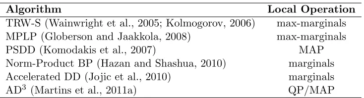
A class of methods that proved effective for approximate inference is based on linear pro-gramming relaxations of the MAP problem (LP-MAP; Schlesinger 1976). Several message-passing and dual decomposition algorithms have been proposed to address the resulting LP problems, taking advantage of the underlying graph structure (Wainwright et al., 2005; Kolmogorov, 2006; Werner, 2007; Komodakis et al., 2007; Globerson and Jaakkola, 2008; Jojic et al., 2010). All these algorithms have a similar consensus-based architecture: they repeatedly perform certain “local” operations in the graph (as outlined in Table 1), until some form of local agreement is achieved. The simplest example is theprojected subgradient dual decomposition (PSDD) algorithm of Komodakis et al. (2007), which has recently en-joyed great success in NLP applications (see Rush and Collins 2012 and references therein). The major drawback of PSDD is that it is too slow to achieve consensus in large problems, requiring O(1/2) iterations for an -accurate solution. While block coordinate descent schemes are usually faster to make progress (Globerson and Jaakkola, 2008), they may get stuck in suboptimal solutions, due to the non-smoothness of the dual objective function. Smoothing-based approaches (Jojic et al., 2010; Hazan and Shashua, 2010) do not have these drawbacks, but in turn they typically involve adjusting a “temperature” parameter for trading off the desired precision level and the speed of convergence, and may suffer from numerical instabilities in the near-zero temperature regime.
In this paper, we present a new LP-MAP algorithm called AD3 (alternating directions dual decomposition), which allies the modularity of dual decomposition with the effective-ness of augmented Lagrangian optimization, via the alternating directions method of mul-tipliers (Glowinski and Marroco, 1975; Gabay and Mercier, 1976). AD3 has an iteration bound ofO(1/), an order of magnitude better than the PSDD algorithm. Like PSDD, AD3
alternates between a broadcast operation, where subproblems are assigned to local
work-ers, and a gather operation, where the local solutions are assembled by a controller, which produces an estimate of the global solution. The key difference is that AD3 regularizes their local subproblems toward these global estimate, which has the effect of speeding up consensus. In many cases of interest, there are closed-form solutions or efficient procedures for solving the AD3 local subproblems (which are quadratic). For factors lacking such a solution, we introduce anactive set method which requires only a local MAP decoder (the same requirement as in PSDD). This paves the way for using AD3 with dense or structured factors.
Our main contributions are:
• We derive AD3 and establish its convergence properties, blending classical and newer results about ADMM (Eckstein and Bertsekas, 1992; Boyd et al., 2011; Wang and Banerjee, 2012). We show that the algorithm has the same form as the PSDD method of Komodakis et al. (2007), with the local MAP subproblems replaced by quadratic
programs. We also show that AD3can be wrapped into a branch-and-bound procedure
Algorithm Local Operation
TRW-S (Wainwright et al., 2005; Kolmogorov, 2006) max-marginals
MPLP (Globerson and Jaakkola, 2008) max-marginals
PSDD (Komodakis et al., 2007) MAP
Norm-Product BP (Hazan and Shashua, 2010) marginals
Accelerated DD (Jojic et al., 2010) marginals
AD3 (Martins et al., 2011a) QP/MAP
Table 1: Several LP-MAP inference algorithms and the kind of the local operations they need to perform at the factors to pass messages and compute beliefs. Some of these operations are the same as the classic loopy BP algorithm, which needs marginals (sum-product variant) or max-marginals (max-product variant). In Section 6, we
will see that the quadratic problems (QP) required by AD3 can be solved as a
sequence of local MAP problems.
• We show that these AD3 subproblems can be solved exactly and efficiently in many
cases of interest, including Ising models and a wide range of hard factors representing arbitrary constraints in first-order logic. Up to a logarithmic term, the asymptotic cost in these cases is the same as that of passing messages or doing local MAP inference.
• For factors lacking a closed-form solution of the AD3 subproblems, we introduce a new
active set method. All is required is a black box that returns local MAP configurations for each factor (the same requirement of the PSDD algorithm). This paves the way for using AD3 with large dense or structured factors, based on off-the-shelf combinatorial algorithms (e.g., Viterbi or Chu-Liu-Edmonds).
AD3 was originally introduced by Martins et al. (2010, 2011a) (then called DD-ADMM). In addition to a considerably more detailed presentation, this paper contains contributions that substantially extend that preliminary work in several directions: the O(1/) rate of convergence, the active set method for general factors, and the branch-and-bound procedure for exact MAP inference. It also reports a wider set of experiments and the release of
open-source code (available athttp://www.ark.cs.cmu.edu/AD3), which may be useful to other
researchers in the field.
2. Background
We start by providing some background on inference in graphical models.
2.1 Factor Graphs
Let Y1, . . . , YM be random variables describing a structured output, with each Yi taking
values in a finite set Yi. We follow the common assumption in structured prediction that
some of these variables have strong statistical dependencies. In this article, we use factor graphs (Tanner, 1981; Kschischang et al., 2001), a convenient way of representing such dependencies that captures directly the factorization assumptions in a model.
Definition 1 (Factor graph) A factor graph is a bipartite graph G := (V, F, E), com-prised of:
• a set of variable nodes V :={1, . . . , M}, corresponding to the variables Y1, . . . , YM; • a set of factor nodes F (disjoint from V);
• a set of edges E ⊆V ×F linking variable nodes to factor nodes.
For notational convenience, we use Latin letters (i, j, ...) and Greek letters (α, β, ...) to refer to variable and factor nodes, respectively. We denote by ∂(·) the neighborhood set of its node argument, whose cardinality is called the degree of the node. Formally, ∂(i) :={α ∈ F |(i, α) ∈E}, for variable nodes, and ∂(α) := {i∈V |(i, α) ∈E} for factor nodes. We use the short notation Yα to refer to tuples of random variables, which take values on the
product set Yα:=Qi∈∂(α)Yi.
We say that the joint probability distribution of Y1, . . . , YM factors according to the
factor graphG= (V, F, E) if it can be written as
P(Y1=y1, . . . , YM =yM) ∝ exp
X
i∈V
θi(yi) +
X
α∈F
θα(yα)
!
, (1)
where θi(·) and θα(·) are called, respectively, the unary and higher-order log-potential
functions.1 To accommodate hard constraints, we allow these functions to take values in ¯
R:=R∪ {−∞}, but we require them to beproper (i.e., they cannot take the value −∞in
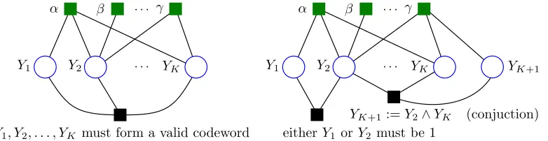
their whole domain). Figure 1 shows examples of factor graphs with hard constraint factors (to be studied in detail in Section 5.2).
2.2 MAP Inference
Given a probability distribution specified as in (1), we are interested in finding an assignment with maximal probability (the so-called MAP assignment/configuration):
b
y1, . . . ,ybM ∈ arg max
y1,...,yM
X
i∈V
θi(yi) +
X
α∈F
θα(yα). (2)
Figure 1: Constrained factor graphs, with soft factors shown as green squares above the variable nodes (circles) and hard constraint factors as black squares below the variable nodes. Left: a global factor that constrains the set of admissible outputs to a given codebook. Right: examples of declarative constraints; one of them is a factor connecting existing variables to an extra variable, allows scores depending on a logical functions of the former.
In fact, this problem is not specific to probabilistic models: other models, e.g., trained to maximize margin, also lead to maximizations of the form above. Unfortunately, for a general factor graphG, this combinatorial problem is NP-hard (Koller and Friedman, 2009), so one must resort to approximations. In this paper, we address a class of approximations based on linear programming relaxations, described formally in the next section.
Throughout the paper, we will make the following assumption:
Assumption 2 The MAP problem (2) is feasible, i.e., there is at least one assignment
y1, . . . , yM such thatPi∈V θi(yi) +
P
α∈Fθα(yα)>−∞.
Note that Assumption 2 is substantially weaker than other assumptions made in the lit-erature on graphical models, which sometimes require the solution of to be unique, or the log-potentials to be all finite. We will see in Section 4 that this is all we need for AD3 to
be globally convergent.
2.3 LP-MAP Inference
Schlesinger’s linear relaxation (Schlesinger, 1976; Werner, 2007) is the building block for many popular approximate MAP inference algorithms. Let us start by representing the log-potential functions in vector notation,θi := (θi(yi))yi∈Yi ∈R¯
|Yi|andθ
α:= (θα(yα))yα∈Yα ∈
¯
R|Yα|. We introduce “local” probability distributions over the variables and factors,
repre-sented as vectors of the same size:
pi ∈∆|Yi|, ∀i∈V and q
α ∈∆|Yα|, ∀α∈F,
where ∆K := {u ∈ RK |u ≥ 0, 1>u = 1} denotes the K-dimensional probability
sim-plex. We stack these distributions into vectors p and q, with dimensions P := P
i∈V |Yi|
and Q := P
α∈F|Yα|, respectively. If these local probability distributions are “valid”
P(Y1, . . . , YM)), then a necessary (but not sufficient) condition is that they arelocally
con-sistent. In other words, they must satisfy the followingcalibration equations: X
yα∼yi
qα(yα) =pi(yi), ∀yi∈Yi, ∀(i, α)∈E, (3)
where the notation ∼ means that the summation is over all configurations yα whose ith
element equalsyi. Equation (3) can be written in vector notation asMiαqα=pi, ∀(i, α)∈ E, where we define consistency matrices
Miα(yi,yα) =
1, ifyα∼yi
0, otherwise.
The set of locally consistent distributions forms the local polytope:
L(G) = (
(p,q)∈RP+Q
qα ∈∆|Yα|, ∀α∈F
Miαqα =pi, ∀(i, α)∈E
)
. (4)
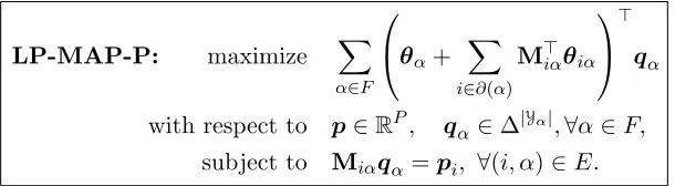
We consider the following linear program (the LP-MAP inference problem):
LP-MAP: maximize X
α∈F
θα>qα+
X
i∈V
θi>pi
with respect to (p,q)∈L(G).
(5)
If the solution (p∗,q∗) of problem (5) happens to be integral, then eachp∗i and q∗α will be at corners of the simplex, i.e., they will be indicator vectors of local configurations yi∗ and y∗α, in which case the output (yi∗)i∈V is guaranteed to be a solution of the MAP decoding
problem (2). Under certain conditions—for example, when the factor graph G does not
have cycles—problem (5) is guaranteed to have integral solutions. In general, however, the LP-MAP decoding problem (5) is a relaxation of (2). Geometrically, L(G) is an outer approximation of the marginal polytope, defined as the set of valid marginals (Wainwright and Jordan, 2008). This is illustrated in Figure 2.
2.4 LP-MAP Inference Algorithms
While any off-the-shelf LP solver can be used for solving problem (5), specialized algorithms have been designed to exploit the graph structure, achieving superior performance on several benchmarks (Yanover et al., 2006). Some of these algorithms are listed in Table 1. Most of these specialized algorithms belong to two classes: block (dual) coordinate descent, which take the form ofmessage-passing algorithms, and projected subgradient algorithms, based on dual decomposition.
Figure 2: Marginal polytope (in green) and its outer approximation, the local polytope (in blue). Each element of the marginal polytope corresponds to a joint distribution of Y1, . . . , YM, and each vertex corresponds to a configuration y ∈ Y, having
coordinates in{0,1}. The local polytope may have additional fractional vertices, with coordinates in [0,1].
the relaxation is tight. A disadvantage of coordinate descent algorithms is that they may get stuck at suboptimal solutions (Bertsekas et al. 1999, Section 6.3.4), since the dual ob-jective is non-smooth (cf. equation (8) below). An alternative is to optimize the dual with the projected subgradient method, which is globally convergent (Komodakis et al., 2007),
and requires computinglocal MAP configurations as its subproblems. Finally,
smoothing-based approaches, such as the accelerated dual decomposition method of Jojic et al. (2010) and the norm-product algorithm of Hazan and Shashua (2010), smooth the dual objective with an en tropic regularization term, leading to subproblems that involve computinglocal marginals.
In Section 8, we discuss advantages and disadvantages of these and other LP-MAP inference methods with respect to AD3.
3. Dual Decomposition with the Projected Subgradient Algorithm
We now describe theprojected subgradient dual decomposition (PSDD) algorithm proposed
by Komodakis et al. (2007). As we will see in Section 4, there is a strong affinity between PSDD and the main focus of this paper, AD3.
Let us first reparameterize (5) to express it as a consensus problem. For each edge (i, α)∈ E, we define a potential functionθiα := (θiα(yi))yi∈Yi that satisfies
P
α∈∂(i)θiα =
θi; a trivial choice isθiα =|∂(i)|−1θi, which spreads the unary potentials evenly across the
factors. Since we have a equality constraint pi =Miαqα, problem (5) is equivalent to the
followingprimal formulation:
LP-MAP-P: maximize X
α∈F
θα+
X
i∈∂(α)
M>iαθiα
>
qα
with respect to p∈RP, qα ∈∆|Yα|,∀α∈F,
subject to Miαqα=pi, ∀(i, α)∈E.
(6)
that the marginals encoded in theq-variables are consistent on their overlaps. Indeed, it is this set of constraints that complicate the optimization problem, which would otherwise be separable into independent subproblems, one per factor. Introducing Lagrange multipliers λiα := (λiα(yi))yi∈Yi for each of these equality constraints leads to the Lagrangian function
L(q,p,λ) = X
α∈F
θα+ X
i∈∂(α)
M>iα(θiα+λiα)
>
qα− X
(i,α)∈E
λiα>pi, (7)
the maximization of which w.r.t. qand pwill yield the (Lagrangian) dual objective. Since thep-variables are unconstrained, we have
max
q,p L(q,p,λ) =
g(λ) ifλ∈Λ,
+∞ otherwise,
and we arrive at the following dual formulation:
LP-MAP-D: minimize g(λ) := X
α∈F gα(λ)
with respect to λ∈Λ,
(8)
where Λ := n
λ | P
α∈∂(i)λiα =0, ∀i∈V
o
is a linear subspace, and each gα(λ) is the
solution of alocal subproblem:
gα(λ) := max
qα∈∆|Yα|
θα+ X
i∈∂(α)
M>iα(θiα+λiα)
>
qα
= max
yα∈Yα
θα(yα) + X
i∈∂(α)
(θiα(yi) +λiα(yi))
; (9)
the last equality is justified by the fact that maximizing a linear objective over the prob-ability simplex gives the largest component of the score vector. Note that the local
sub-problem (9) can be solved by aComputeMAPprocedure, which receives unary potentials
ξiα(yi) :=θiα(yi)+λiα(yi) and factor potentialsθα(yα) (eventually structured) and returns
the MAPybα.
Problem (8) is often referred to as themaster orcontroller, and each local subproblem (9) as aslave orworker. The master problem (8) can be solved with aprojected subgradient algorithm.2 By Danskin’s rule (Bertsekas et al., 1999, p. 717), a subgradient ofgαis readily
given by
∂gα(λ) ∂λiα
=Miαbqα, ∀(i, α)∈E;
and the projection onto Λ amounts to a centering operation. Putting these pieces together yields Algorithm 1. At each iteration, the algorithm broadcasts the current Lagrange mul-tipliers to all the factors. Each factor adjusts its internal unary log-potentials (line 6) and
Algorithm 1 PSDD Algorithm (Komodakis et al., 2007)
1: input: graph G, parametersθ, maximum number of iterationsT, step sizes (ηt)Tt=1 2: for each (i, α)∈E, choose θiα such that Pα∈∂(i)θiα =θi
3: initializeλ=0 4: fort= 1 toT do
5: for each factorα∈F do
6: set unary log-potentialsξiα:=θiα+λiα, fori∈∂(α)
7: setbqα:=ComputeMap(θα+Pi∈∂(α)M>iαξiα)
8: setbqiα:=Miαqbα, fori∈∂(α)
9: end for
10: compute averagepi :=|∂(i)|−1P
α∈∂(i)bqiα for each i∈V
11: updateλiα :=λiα−ηt(bqiα−pi) for each (i, α)∈E
12: end for
13: output: dual variable λand upper boundg(λ)
invokes the ComputeMap procedure (line 7).3 The solutions achieved by each factor are
then gathered and averaged (line 10), and the Lagrange multipliers are updated with step size ηt (line 11). The two following propositions establish the convergence properties of
Algorithm 1.
Proposition 3 (Convergence rate) If the non-negative step size sequence(ηt)t∈N is di-minishing and nonsummable (limηt = 0 and
P∞
t=1ηt = ∞), then Algorithm 1 converges
to the solution λ∗ of LP-MAP-D (8). Furthermore, after T =O(1/2) iterations, we have
g(λ(T))−g(λ∗)≤.
Proof: This is a property of projected subgradient algorithms (see, e.g., Bertsekas et al. 1999).
Proposition 4 (Certificate of optimality) If, at some iteration of Algorithm 1, all the local subproblems are in agreement (i.e., ifbqiα =pi after line 10, for alli∈V), then: (i)λ
is a solution of LP-MAP-D (8); (ii) p is binary-valued and a solution of both LP-MAP-P and MAP.
Proof: If all local subproblems are in agreement, then a vacuous update will occur in line 11, and no further changes will occur. Since the algorithm is guaranteed to converge, the current λ is optimal. Also, if all local subproblems are in agreement, the averaging in line 10 necessarily yields a binary vector p. Since any binary solution of LP-MAP is also a solution of MAP, the result follows.
Propositions 3–4 imply that, if the LP-MAP relaxation is tight, then Algorithm 1 will eventually yield the exact MAP configuration along with a certificate of optimality. Ac-cording to Proposition 3, even if the relaxation is not tight, Algorithm 1 still converges to
3. Note that, if the factor log-potentialsθαhave special structure (e.g., if the factor is itself combinatorial,
such as a sequence or a tree model), then this structure is preserved since only the internal unary log-potentials are changed. Therefore, if evaluating ComputeMap(θα) is tractable, so is evaluating
a solution of LP-MAP. Unfortunately, in large graphs with many overlapping factors, it has been observed that convergence can be quite slow in practice (Martins et al., 2011b). This is not surprising, given that it attempts to reach a consensus among all overlapping components; the larger this number, the harder it is to achieve consensus. We describe in the next section another LP-MAP decoder (AD3) with a faster convergence rate.
4. Alternating Directions Dual Decomposition (AD3)
AD3 avoids some of the weaknesses of PSDD by replacing the subgradient method with the
alternating directions method of multipliers(ADMM). Before going into a formal derivation, let us go back to the PSDD algorithm to pinpoint the crux of its weaknesses. It resides in two aspects:
1. The dual objective function g(λ) is non-smooth, this being why “subgradients” are used instead of “gradients.” It is well-known that non-smooth optimization lacks some of the good properties of its smooth counterpart. Namely, there is no guarantee of monotonic improvement in the objective (see Bertsekas et al. 1999, p. 611). Ensuring convergence requires using a diminishing step size sequence, which leads to slow con-vergence rates. In fact, as stated in Proposition 3,O(1/2) iterations are required to
guarantee-accuracy.
2. A close look at Algorithm 1 reveals that the consensus is promoted solely by the Lagrange multipliers (line 6). These can be regarded as “price adjustments” that are made at each iteration and lead to a reallocation of resources. However, no “memory” exists about past allocations or adjustments, so the workers never know how far they are from consensus. One may suspect that a smarter use of these quantities may accelerate convergence.
The first of these aspects has been addressed by the accelerated dual decomposition method of Jojic et al. (2010), which improves the iteration bound toO(1/); we discuss that work further in Section 8. We will see that AD3 also yields a O(1/) iteration bound with some additional advantages. The second aspect is addressed by AD3 by broadcastingthe current global solution in addition to the Lagrange multipliers, allowing the workers to regularize their subproblems toward that solution.
4.1 Augmented Lagrangians and the Alternating Directions Method of Multipliers
Let us start with a brief overview of augmented Lagrangian methods. Consider the following general convex optimization problem with equality constraints:
maximize f1(q) +f2(p)
with respect to q∈Q,p∈P
subject to Aq+Bp=c,
(10)
where Q ⊆RP and P ⊆ RQ are convex sets and f1 :Q → R¯ and f2 :P → R¯ are concave
consider the problem
maximize f1(q) +f2(p)−η2kAq+Bp−ck2
with respect to q∈Q,p∈P
subject to Aq+Bp=c,
(11)
which differs from (10) in the extra term penalizing violations of the equality constraints; since this term vanishes at feasibility, the two problems have the same solution. The La-grangian of (11),
Lη(q,p,λ) =f1(q) +f2(p) +λ>(Aq+Bp−c)−
η
2kAq+Bp−ck
2,
is called theη-augmented Lagrangianof (10). The so-calledaugmented Lagrangianmethods (Bertsekas et al., 1999, Section 4.2) address problem (10) by seeking a saddle point ofLηt,
for some sequence (ηt)t∈N. The earliest instance is the method of multipliers (Hestenes,
1969; Powell, 1969), which alternates between a joint update ofq and pthrough
(qt+1,pt+1) := arg max
q,p {Lηt(q,p,λ
t) |q∈Q,p∈P} (12)
and a gradient update of the Lagrange multiplier,
λt+1 := λt−ηt(Aqt+1+Bpt+1−c).
Under some conditions, this method is convergent, and even superlinear, if the sequence (ηt)t∈N is increasing (Bertsekas et al. 1999, Section 4.2). A shortcoming of this method is
that problem (12) may be difficult, since the penalty term of the augmented Lagrangian
couples the variables p and q. The alternating directions method of multipliers (ADMM)
avoids this shortcoming, by replacing the joint optimization (12) by a single block Gauss-Seidel-type step:
qt+1:= arg max
q∈Q Lηt(q,p
t,λt) = arg max
q∈Q f1(q) + (A
>λt)>q−ηt
2kAq+Bp
t−ck2, (13)
pt+1:= arg max p∈P Lηt(q
t+1,p,λt) = arg max
p∈P f2(p) + (B
>λt)>p−ηt
2kAq
t+1+Bp−ck2. (14)
In general, problems (13)–(14) are simpler than the joint maximization in (12). ADMM was proposed by Glowinski and Marroco (1975) and Gabay and Mercier (1976) and is related to other optimization methods, such as Douglas-Rachford splitting (Eckstein and Bertsekas, 1992) and proximal point methods (see Boyd et al. 2011 for an historical overview).
4.2 Derivation of AD3
Our LP-MAP-P problem (6) can be cast into the form (10) by proceeding as follows:
• let Qin (10) be the Cartesian product of simplices, Q:=Q
α∈F∆
|Yα|, andP:=
RP;
• let f1(q) :=Pα∈F
θα+Pi∈∂(α)M>iαθiα
>
• let A in (10) be a R×Q block-diagonal matrix, where R =P
(i,α)∈E|Yi|, with one
block per factor, which is a vertical concatenation of the matrices{Miα}i∈∂(α);
• let −B be a R×P matrix of grid-structured blocks, where the block in the (i, α)th row and the ith column is a negative identity matrix of size |Yi|, and all the other blocks are zero;
• let c:= 0.
The η-augmented Lagrangian associated with (6) is
Lη(q,p,λ) =
X
α∈F
θα+
X
i∈∂(α)
M>iα(θiα+λiα)
>
qα− X
(i,α)∈E
λiα>pi− η 2
X
(i,α)∈E
kMiαqα−pik2.
This is the standard Lagrangian (7) plus the Euclidean penalty term. The ADMM updates are
Broadcast: q(t):= arg max
q∈Q Lηt(q,p
(t−1),λ(t−1)), (15) Gather: p(t) := arg max
p∈RP
Lηt(q
(t),p,λ(t−1)), (16) Multiplier update: λ(iαt) :=λ(iαt−1)−ηt
Miαq(αt)−p
(t)
i
,∀(i, α)∈E. (17)
We next analyze the broadcast and gather steps, and prove a proposition about the multi-plier update.
4.2.1 Broadcast Step
The maximization (15) can be carried out in parallel at the factors, as in PSDD. The only difference is that, instead of a local MAP computation, each worker now needs to solve a
quadratic program of the form:
max qα∈∆|Yα|
θα+ X
i∈∂(α)
M>iα(θiα+λiα)
>
qα−η 2
X
i∈∂(α)
kMiαqα−pik2. (18)
4.2.2 Gather Step
The solution of problem (16) has a closed form. Indeed, this problem is separable into independent optimizations, one for eachi∈V; defining qiα :=Miαqα,
p(it) := arg min pi∈R|Yi|
X
α∈∂(i)
pi− qiα−ηt−1λiα
2
= |∂(i)|−1 X α∈∂(i)
qiα−η−t1λiα
= 1
|∂(i)| X
α∈∂(i)
qiα.
The equality in the last line is due to the following proposition:
Proposition 5 The sequence λ(1),λ(2), . . . produced by the updates (15)–(17) is dual fea-sible, i.e., we have λ(t)∈Λ for everyt, withΛ as in (8).
Proof: We have:
X
α∈∂(i)
λ(iαt)= X
α∈∂(i)
λ(iαt−1)−ηt
X
α∈∂(i)
q(iαt)− |∂(i)|p(it)
= X
α∈∂(i)
λ(iαt−1)−ηt
X
α∈∂(i)
q(iαt)− X α∈∂(i)
qiα(t)−ηt−1λ(iαt−1)
=0.
Assembling all these pieces together leads to AD3 (Algorithm 2), where we use a fixed step sizeη. Notice that AD3retains the modular structure of PSDD (Algorithm 1). The key difference is that AD3 also broadcasts the current global solution to the workers, allowing them to regularize their subproblems toward that solution, thus speeding up the consensus.
This is embodied in the procedure SolveQP (line 7), which replaces ComputeMAP of
Algorithm 1.
4.3 Convergence Analysis
Before proving the convergence of AD3, we start with a basic result.
Proposition 6 (Existence of a Saddle Point) Under Assumption 2, we have the fol-lowing properties (regardless of the choice of log-potentials):
1. LP-MAP-P (6)is primal-feasible;
2. LP-MAP-D (8)is dual-feasible;
3. The Lagrangian functionL(q,p,λ)has a saddle point(q∗,p∗,λ∗)∈Q×P×Λ, where
Algorithm 2 Alternating Directions Dual Decomposition (AD3)
1: input: graph G, parametersθ, penalty constant η
2: initializepuniformly (i.e., pi(yi) = 1/|Yi|,∀i∈V, yi ∈Yi)
3: initializeλ=0
4: repeat
5: for each factor α∈F do
6: set unary log-potentialsξiα:=θiα+λiα, fori∈∂(α)
7: setbqα:=SolveQP
θα+Pi∈∂(α)M >
iαξiα, (pi)i∈∂(α)
8: setbqiα:=Miαqbα, fori∈∂(α)
9: end for
10: compute averagepi :=|∂(i)|−1P
α∈∂(i)bqiα for each i∈V
11: updateλiα :=λiα−η(bqiα−pi) for each (i, α)∈E
12: untilconvergence
13: output: primal variablesp and q, dual variable λ, upper boundg(λ)
Proof: Property 1 follows directly from Assumption 2 and the fact that LP-MAP is a relaxation of MAP. To prove properties 2–3, define first the set of structural constraints ¯Q:= Q
α∈FQ¯α, where ¯Qα := {qα ∈ ∆|Yα| |qα(yα) = 0,∀yα s.t. θα(yα) = −∞} are truncated
probability simplices (hence convex). Since all log-potential functions are proper (due to Assumption 2), we have that each ¯Qα is non-empty, and therefore ¯Qhas non-empty relative
interior. As a consequence, the refined Slater’s condition (Boyd and Vandenberghe, 2004, §5.2.3) holds; let (q∗, p∗) ∈Q¯×Pbe a primal feasible solution of LP-MAP-P, which exists by virtue of property 1. Then, the KKT optimality conditions imply the existence of a λ∗ such that (q∗,p∗,λ∗) is a saddle point of the Lagrangian function L, i.e., L(q,p,λ∗)≤ L(q∗,p∗,λ∗)≤L(q∗,p∗,λ) holds for allq,p,λ. Naturally, we must haveλ∗∈Λ, otherwise L(., .,λ∗) would be unbounded with respect to p.
We are now ready to show the convergence of AD3, which follows directly from the
general convergence properties of ADMM. Remarkably, unlike in PSDD, convergence is ensured with a fixed step size, therefore no annealing is required.
Proposition 7 (Convergence of AD3) Let (q(t),p(t),λ(t))t be the sequence of iterates
produced by Algorithm 2 with a fixedηt=η. Then the following holds:
1. primal feasibility of LP-MAP-P (6)is achieved in the limit, i.e.,
kMiαq(αt)−p
(t)
i k →0, ∀(i, α)∈E;
2. the primal objective sequenceP
i∈V θi>p(it)+
P
α∈Fθα>q(αt)
t∈Nconverges to the so-lution of LP-MAP-P (6);
3. the dual sequence (λ(t))t∈N converges to a solution of the dual LP-MAP-D (8); more-over, this sequence is dual feasible, i.e., it is contained in Λ. Thus, g(λ(t)) in (8)
Proof: See Boyd et al. (2011, Appendix A) for a simple proof of the convergence of ADMM in the form (10), from which 1, 2, and the first part of 3 follow immediately. The two assumptions stated in Boyd et al. (2011, p.16) are met: denoting by ιQ the indicator
function of the set Q, which evaluates to zero in Q and to −∞ outside Q, we have that
functions f1 +ιQ and f2 are closed proper convex (since the log-potential functions are
proper and f1 is closed proper convex), and the unaugmented Lagrangian has a saddle
point (see property 3 in Proposition 6). Finally, the last part of statement 3 follows from Proposition 5.
The next proposition, proved in Appendix A, states theO(1/) iteration bound of AD3, which is better than theO(1/2) bound of PSDD.
Proposition 8 (Convergence rate of AD3) Assume the conditions of Proposition 7. Let λ∗ be a solution of the dual problem (8), λ¯T := T1 PTt=1λ(t) be the “averaged” La-grange multipliers after T iterations of AD3, and g(¯λT) the corresponding estimate of the
dual objective (an upper bound). Then, g(¯λT)−g(λ∗)≤ after T ≤C/ iterations, where C is a constant satisfying
C ≤ 5η
2 X
i∈V
|∂(i)| ×(1− |Yi|−1) + 5
2ηkλ
∗k2
≤ 5η
2 |E|+
5 2ηkλ
∗k2. (19)
As expected, the bound (19) increases with the number of overlapping variables, quan-tified by the number of edges |E|, and the magnitude of the optimal dual vectorλ∗. Note that if there is a good estimate of kλ∗k, then (19) can be used to choose a step size η that minimizes the bound—the optimal step size is η = kλ∗k × |E|−1/2, which would lead to
T ≤5−1|E|1/2kλ∗k. In fact, although Proposition 7 guarantees convergence for any choice
of η, we observed in practice that this parameter has a strong impact on the behavior of the algorithm. In our experiments, we dynamically adjust η in earlier iterations using the heuristic described in Boyd et al. (2011, Section 3.4.1), and freeze it afterwards, not to compromise convergence.
4.4 Stopping Conditions and Implementation Details
We next establish stopping conditions for AD3 and discuss some implementation details
that can provide significant speed-ups.
4.4.1 Primal and Dual Residuals
terminate when a near optimal relaxed primal solution has been found.4 This is an impor-tant advantage over PSDD, which is unable to provide similar stopping conditions, and is usually stopped rather arbitrarily after a given number of iterations.
The primal residual rP(t) is the amount by which the agreement constraints are violated,
r(Pt)= P
(i,α)∈EkMiαqα(t)−p(it)k2
P
(i,α)∈E|Yi|
∈[0,1],
where the constant in the denominator ensures thatr(Pt)∈[0,1]. Thedual residual r(Dt),
rD(t)= P
(i,α)∈Ekp
(t)
i −p
(t−1)
i k2
P
(i,α)∈E|Yi|
∈[0,1],
is the amount by which a dual optimality condition is violated (see Boyd et al. 2011, §3.3 for details). We adopt as stopping criterion that these two residuals fall below a threshold, e.g., 10−6.
4.4.2 Approximate Solutions of the Local Subproblems
The next proposition states that convergence may still hold if the local subproblems are only solved approximately. The importance of this result will be clear in Section 6, where we describe a general iterative algorithm for solving the local quadratic subproblems. Essen-tially, Proposition 9 allows these subproblems to be solved numerically up to some accuracy without compromising global convergence, as long as the accuracy of the solutions improves sufficiently fast over AD3 iterations.
Proposition 9 (Eckstein and Bertsekas, 1992) Let ηt = η, and for each iteration t,
let bq(t) contain the exact solutions of (18), and q˜(t) those produced by an approximate algorithm. Then Proposition 7 still holds, provided that the sequence of errors is summable, i.e.,P∞
t=1kbq
(t)−˜
q(t)k<∞.
4.4.3 Runtime and Caching Strategies
In practice, considerable speed-ups can be achieved by caching the subproblems, a strategy which has also been proposed for the PSDD algorithm by Koo et al. (2010). After a few iterations, many variables pi reach a consensus (i.e., p(it) = qiα(t+1),∀α ∈ ∂(i)) and enter an idle state: they are left unchanged by the p-update (line 10), and so do the Lagrange variables λ(iαt+1) (line 11). If at iteration t all variables in a subproblem at factor α are idle, then q(αt+1) = q(αt), hence the corresponding subproblem does not need to be solved.
Typically, many variables and subproblems enter this idle state after the first few rounds. We will show the practical benefits of caching in the experimental section (Section 7.4, Figure 9).
4. This is particularly useful if inference is embedded in learning, where it is more important to obtain a
fractional solution of the relaxed primal than an approximate integer one (Kulesza and Pereira, 2007;
4.5 Exact Inference with Branch-and-Bound
Recall that AD3, as just described, solves the LP-MAP relaxation of the actual problem. In some problems, this relaxation is tight (in which case a certificate of optimality will be obtained), but this is not always the case. When a fractional solution is obtained, it is desirable to have a strategy to recover the exact MAP solution.
Two observations are noteworthy. First, as we saw in Section 2.3, the optimal value of the relaxed problem LP-MAP provides an upper bound to the original problem MAP. In particular, any feasible dual point provides an upper bound to the original problem’s optimal value. Second, during execution of the AD3 algorithm, we always keep track of a sequence of feasible dual points (as guaranteed by Proposition 7, item 3. Therefore, each iteration constructs tighter and tighter upper bounds. In recent work (Das et al., 2012), we proposed abranch-and-bound search procedure that finds the exact solution of the ILP. The procedure works recursively as follows:
1. Initialize L=−∞(our best value so far).
2. Run Algorithm 2. If the solution p∗ is integer, return p∗ and set L to the objective value. If along the execution we obtain an upper bound less thanL, then Algorithm 2 can be safely stopped and return “infeasible”—this is the bound part. Otherwise (if p∗ is fractional) go to step 3.
3. Find the “most fractional” component of p∗ (call it p∗j(.)) and branch: for every yj ∈ Yj, create a branch where pj(yj) = 1 and pj(yj0) = 0 for yj0 6= yj, and go
to step 2, eventually obtaining an integer solution p∗|yj or infeasibility. Return the
p∗∈ {p∗|yj}yj∈Yj that yields the largest objective value.
Although this procedure has worst-case exponential runtime, in many problems for which the relaxations are near-exact it is found empirically very effective. We will see one example in Section 7.3.
5. Local Subproblems in AD3
This section shows how to solve the AD3 local subproblems (18) exactly and efficiently, in several cases, including Ising models and logic constraint factors. These results will be
complemented in Section 6, where a new procedure to handle arbitrary factors widens the
applicability of AD3. By subtracting a constant, re-scaling, and flipping signs, problem (18) can be written more compactly as
minimize 1
2kMqα−ak
2−b>q
α (20)
with respect to qα∈R|Yα|
subject to 1>qα= 1, qα≥0,
where a:= (ai)i∈∂(α), with ai :=pi+η−1(θiα +λiα); b:= η−1θα; and M:= (Miα)i∈∂(α)
denotes a matrix withP
i|Yi|rows and|Yα|columns.
(FOL) constraints, and for Potts models (after binarization). In these cases, AD3 and the PSDD algorithm have (asymptotically) the same computational cost per iteration, up to a logarithmic factor.
5.1 Ising Models
Ising models are factor graphs containing only binary pairwise factors. A binary pairwise factor (say,α) is one connecting two binary variables (say,Y1andY2); thusY1 =Y2 ={0,1}
and Yα = {00,01,10,11}. Given that q1α,q2α ∈ ∆2, we can write q1α = (1 −z1, z1),
q2α= (1−z2, z2). Furthermore, sinceqα ∈∆4 and marginalization requires thatqα(1,1) + qα(1,0) = z1 and qα(0,1) +qα(1,1) = z2, we can also writeqα = (1−z1 −z2+z12, z1−
z12, z2−z12, z12). Using this parameterization, problem (20) reduces to:
minimize 1
2(z1−c1)
2+ 1
2(z2−c2)
2−c 12z12
with respect to z1, z2, z12∈[0,1]3
subject to z12≤z1, z12≤z2, z12≥z1+z2−1, (21)
where
c1 =
a1α(1) + 1−a1α(0)−bα(0,0) +bα(1,0)
2
c2 =
a2α(1) + 1−a2α(0)−bα(0,0) +bα(0,1)
2
c12 =
bα(0,0)−bα(1,0)−bα(0,1) +bα(1,1)
2 .
The next proposition (proved in Appendix B.1) establishes a closed form solution for this
problem, which immediately translates into a procedure for SolveQP for binary pairwise
factors.
Proposition 10 Let [x]U := min{max{x,0},1} denote projection (clipping) onto the unit interval U:= [0,1]. The solution (z1∗, z2∗, z12∗ ) of problem (21) is the following. If c12≥0,
(z∗1, z2∗) =
([c1]U, [c2+c12]U), if c1> c2+c12
([c1+c12]U, [c2]U), if c2> c1+c12
([(c1+c2+c12)/2]U, [(c1+c2+c12)/2]U), otherwise,
z12∗ = min{z1∗, z2∗}; (22)
otherwise ,
(z1∗, z2∗) =
([c1+c12]U, [c2+c12]U), if c1+c2+ 2c12>1
([c1]U, [c2]U), if c1+c2 <1
([(c1+ 1−c2)/2]U, [(c2+ 1−c1)/2]U), otherwise,
5.2 Factor Graphs with First-Order Logic Constraints
Hard constraint factors allow specifying “forbidden” configurations, and have been used in error-correcting decoders (Richardson and Urbanke, 2008), bipartite graph matching (Duchi et al., 2007), computer vision (Nowozin and Lampert, 2009), and natural language processing (Smith and Eisner, 2008). In many applications,declarative constraints are useful for injecting domain knowledge, and first-order logic (FOL) provides a natural language to express such constraints. This is particularly useful in learning from scarce annotated data (Roth and Yih, 2004; Punyakanok et al., 2005; Richardson and Domingos, 2006; Chang et al., 2008; Poon and Domingos, 2009).
In this section, we consider hard constraint factors linked to binary variables, with log-potential functions of the form
θα(yα) =
0, ifyα∈Sα
−∞, otherwise,
where Sα ⊆ {0,1}|∂(α)| is an acceptance set. These factors can be used for imposing FOL
constraints, as we describe next. We define the marginal polytope Zα of a hard constraint
factor α as the convex hull of its acceptance set,
Zα= convSα. (24)
As shown in Appendix B.2, the AD3 subproblem (20) associated with a hard constraint factor is equivalent to that of computing an Euclidean projection onto its marginal polytope:
minimize kz−z0k2
with respect to z∈Zα, (25)
wherez0i := (ai(1)+1−ai(0))/2, fori∈∂(α). We now show how to compute this projection
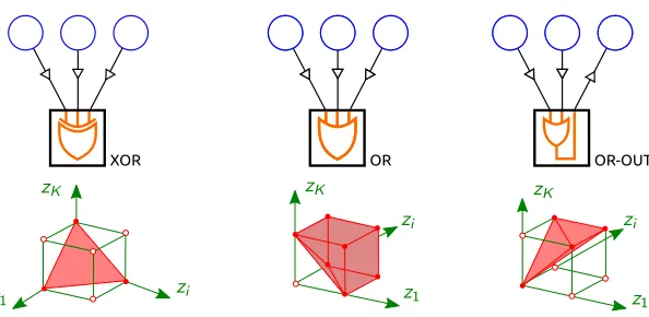
for several hard constraint factors that are building blocks for writing FOL constraints. Each of these factors performs a logical function, and hence we represent them graphically aslogic gates (Figure 3).
5.2.1 One-Hot XOR (Uniqueness Quantification)
The “one-hot XOR” factor linked toK≥1 binary variables is defined through the following potential function:
θXOR(y1, . . . , yK) :=
0 if∃!k∈ {1, . . . , K}s.t. yk = 1
−∞ otherwise,
where ∃! denotes “there is one and only one.” The name “one-hot XOR” stems from the
following fact: forK = 2, exp(θXOR(.)) is the logic eXclusive-OR function; the prefix
XOR OR OR-OUT
Figure 3: Logic factors and their marginal polytopes; the AD3 subproblems (25) are projec-tions onto these polytopes. Left: the one-hot XOR factor (its marginal polytope is the probability simplex). Middle: the OR factor. Right: the OR-with-output factor.
From (24), the marginal polytope associated with the one-hot XOR factor is
ZXOR = conv
y∈ {0,1}K | ∃!k∈ {1, . . . , K}s.t. yk= 1 = ∆K
as illustrated in Figure 3. Therefore, the AD3 subproblem for the XOR factor consists in projecting onto the probability simplex, a problem well studied in the literature (Brucker, 1984; Michelot, 1986; Duchi et al., 2008). In Appendix B.3, we describe a simpleO(KlogK) algorithm. Note that there are O(K) algorithms for this problem which are slightly more involved.
5.2.2 OR (Existential Quantification)
This factor represents a disjunction of K≥1 binary variables,
θOR(y1, . . . , yK) :=
0 if∃k∈ {1, . . . , K}s.t. yk= 1
−∞ otherwise,
The OR factor can be used to represent a statement in FOL of the form ∃x:R(x). From Proposition 16, the marginal polytope associated with the OR factor is:
ZOR = conv
y∈ {0,1}K | ∃k∈ {1, . . . , K}s.t. yk= 1
= (
z∈[0,1]K
K
X
k=1
zk≥1
)
;
geometrically, it is a “truncated” hypercube, as depicted in Figure 3. We derive aO(KlogK) algorithm for projecting onto ZOR, using a sifting technique and a sort operation (see
5.2.3 Logical Variable Assignments: OR-With-Output
The two factors above define a constraint on a group of existing variables. Alternatively, we may want to define a new variable (say,yK+1) which is the result of an operation involving
other variables (say, y1, . . . , yK). Among other things, this will allow dealing with “soft
constraints,” i.e., constraints that can be violated but whose violation will decrease the score by some penalty. An example is the OR-with-output factor:
θOR−out(y1, . . . , yK, yK+1) :=
1 ifyK+1=y1∨ · · · ∨yK
0 otherwise.
This factor constrains the variable yK+1 to indicate the existence of one or more active
variables among y1, . . . , yK. It can be used to express the following statement in FOL: T(x) :=∃z:R(x, z).
The marginal polytope associated with the OR-with-output factor (also depicted in Figure 3):
ZOR−out = conv
y∈ {0,1}K+1
yK+1 =y1∨ · · · ∨yK
= (
z∈[0,1]K+1
K
X
k=1
zk≥zK+1, zk≤zK+1,∀k∈ {1, . . . , K}
)
.
Although projecting onto ZOR−out is slightly more complicated than the previous cases, in
Appendix B.5, we propose (and prove correctness of) anO(KlogK) algorithm for this task.
5.2.4 Negations, De Morgan’s Laws, and AND-With-Output
The three factors just presented can be extended to accommodate negated inputs, thus
adding flexibility. Solving the corresponding AD3subproblems can be easily done by reusing the methods that solve the original problems. For example, it is straightforward to handle negated conjunctions (NAND),
θNAND(y1, . . . , yK) :=
−∞ ifyk= 1,∀k∈ {1, . . . , K}
0 otherwise,
= θOR(¬y1, . . . ,¬yK),
as well as implications (IMPLY),
θIMPLY(y1, . . . , yK, yK+1) :=
0 if (y1∧ · · · ∧yK)⇒yK+1
−∞ otherwise
= θOR(¬y1, . . . ,¬yK, yK+1).
In fact, from De Morgan’s laws, ¬(Q1(x)∧ · · · ∧QK(x)) is equivalent to ¬Q1(x)∨ · · · ∨
¬QK(x), and (Q1(x)∧ · · · ∧QK(x)) ⇒ R(x) is equivalent to (¬Q1(x)∨ · · · ∨ ¬QK(x))∨ R(x). Another example is the AND-with-output factor,
θAND−out(y1, . . . , yK, yK+1) :=
0 ifyK+1=y1∧ · · · ∧yK
−∞ otherwise
which can be used to impose FOL statements of the formT(x) :=∀z:R(x, z).
Letα be a binary constraint factor with marginal polytopeZα, andβ a factor obtained
fromαby negating thekth variable. For notational convenience, let symk: [0,1]K →[0,1]K be defined as (symk(z))k = 1−zk and (symk(z))i = zi, for i 6= k. Then, the marginal
polytope Zβ is a symmetric transformation of Zα,
Zβ =
n
z∈[0,1]K symk(z)∈Zα o
,
and, if projZα denotes the projection operator ontoZα,
projZβ(z) = symk projZα(symk(z)).
Naturally, projZβ can be computed as efficiently as projZα and, by induction, this procedure can be generalized to an arbitrary number of negated variables.
5.3 Potts Models and Graph Binarization
Although general factors lack closed-form solutions of the corresponding AD3 subproblem (20), it is possible tobinarize the graph, i.e., to convert it into an equivalent one that only contains binary variables and XOR factors. The procedure is as follows:
• For each variable node i ∈ V, define binary variables Ui,yi ∈ {0,1}, for each state
yi ∈Yi; link these variables to a XOR factor, imposing Pyi∈Yipi(yi) = 1.
• For each factor α ∈F, define binary variables Uα,yα ∈ {0,1} for everyyα ∈Yα. For
each edge (i, α) ∈E and eachyi ∈Yi, link variables {Uα,yα |yα ∼yi} and ¬Ui,yi to
a XOR factor; this imposes the constraint pi(yi) =Py
α∼yiqα(yα).
The resulting binary graph is one for which we already presented the machinery needed for
solving efficiently the corresponding AD3 subproblems. As an example, for Potts models
(graphs with only pairwise factors and variables that have more than two states), the computational cost per AD3 iteration on the binarized graph is asymptotically the same as that of the PSDD and other message-passing algorithms; for details, see Martins (2012).
6. An Active Set Method For Solving the AD3 Subproblems
In this section, we complement the results of Section 5 with a general active-set procedure
for solving the AD3 subproblems forarbitrary factors, the only requirement being a
black-box MAP solver—the same as the PSDD algorithm. This makes AD3 applicable to a wide
range of problems. In particular, it makes possible to handlestructured factors, by invoking
specialized MAP decoders (functions ComputeMAP in Algorithm 1). In practice, as we
will see in Section 7, the active set method we next present largely outperforms the graph binarization strategy outlined in Section 5.3.
Proposition 11 Problem (20) admits a solution q∗α ∈ R|Yα| with at most P
i∈∂(α)|Yi| − |∂(α)|+ 1non-zero components.
The fact that the solution lies in a low dimensional subspace makes active set methods appealing, since they only keep track of an active set of variables, that is, the non-zero components ofqα. Proposition 11 tells us that such an algorithm only needs to maintain at
most O(P
i|Yi|) elements in the active set—note the additive, rather than multiplicative,
dependency on the number of values of the variables. Our active set method seeks to identify the low-dimensional support of the solution q∗α, by generating sparse iterates q(1)α ,q(2)α , . . .,
while it maintains a working set W ⊆ Yα with the inequality constraints of (20) that are
inactive along the way (i.e., those yα for which qα(yα) >0 holds strictly). Each iteration
adds or removes elements from the working set while it monotonically decreases the objective of (20).5
Lagrangian and KKT conditions. Let τ and µ be dual variables associated with the equality and inequality constraints of (20), respectively. The Lagrangian function is
L(qα, τ,µ) = 1
2kMqα−ak
2−b>q
α−τ(1−1>qα)−µ>qα.
This gives rise to the following Karush-Kuhn-Tucker (KKT) conditions:
M>(a−Mqα) +b=τ1−µ (∇qαL=0) (26)
1>qα= 1, qα ≥0, µ≥0 (Primal/dual feasibility) (27)
µ>qα=0 (Complementary slackness). (28)
The method works at follows. At each iterations, it first checks if the current iterate q(αs)
is a subspace minimizer, i.e., if it optimizes the objective of (20) in the sparse subspace defined by the working set W, {qα ∈ ∆|Yα| |q
α(yα) = 0,∀yα ∈/ W}. This check can be
made by first solving a relaxation where the inequality constraints are ignored. Since in this subspace the components ofqα not inW will be zeros, one can simply delete those entries
from qα and b and the corresponding columns in M; we use a horizontal bar to denote
these truncated R|W|-vectors. The problem can be written as:
minimize 1
2kM¯q¯α−ak
2−¯b>q¯
α
with respect to q¯α∈R|W|
subject to 1>q¯α= 1. (29)
The solution of this equality-constrained QP can be found by solving a system of KKT equations:6
¯
M>M¯ 1 1> 0
¯ qα
τ
= ¯
M>a+ ¯b 1
. (30)
5. Our description differs from Nocedal and Wright (1999) in which their working set contains active
constraints rather than the inactive ones. In our case, most constraints are active for the optimalq∗α,
therefore it is appealing to store the ones that are not.
6. Note that this is a low-dimensional problem, since we are working in a sparse working set. By caching the inverse of the matrix in the left-hand side, this system can be solved in timeO(|W|2
The solution of (30) will give (bqα,bτ), where qbα ∈ R|Yα| is padded back with zeros. If
it happens that bqα = q
(s)
α , then this means that the current iterate q(αs) is a subspace
minimizer; otherwise a new iterate q(αs+1) will be computed. We next discuss these two
events.
• Case 1: q(αs) is a subspace minimizer. If this happens, then it may be the case that
q(αs) is the optimal solution of (20). By looking at the KKT conditions (26)–(28), we
have that this will happen iff M>(a−Mq(αs)) +b≤ τ(s)1. Define w := a−Mqα.
The condition above is equivalent to
max yα∈Yα
b(yα) + X
i∈∂(α)
wi(yi)
≤τ(s).
It turns out that this maximization is precisely alocal MAP inference problem, given a vector of unary potentials w and factor potentials b. Thus, the maximizer byα
can be computed via the ComputeMAP procedure, which we assume available. If
b(ybα) + P
i∈∂(α)wi(ybi)≤τ
(s), then the KKT conditions are satisfied and we are done.
Otherwise,ybα indicates the most violated condition; we will add it to the active set W, and proceed.
• Case 2: q(αs) is not a subspace minimizer. If this happens, then we compute a new
iterate q(αs+1) by keeping searching in the same subspace. We have already solved a
relaxation in (29). If we haveqbα(yα)≥0 for all yα ∈W, then the relaxation is tight,
so we just setq(αs+1) :=bqα and proceed. Otherwise, we move as much as possible in the direction ofbqαwhile keeping feasibility, by definingq
(s+1)
α := (1−β)q(αs)+βbqα—as described in Nocedal and Wright (1999), the value of β ∈ [0,1] can be computed in closed form:
β= min
(
1, min
yα∈W :q (s)
α (yα)>bqα(yα)
qα(s)(yα) qα(s)(yα)−qbα(yα)
)
. (31)
If β < 1, this update will have the effect of making one of the constraints active,
by zeroing out qα(s+1)(yα) for the minimizing yα above. This so-called “blocking
constraint” is thus be removed from the working setW.
Algorithm 3 describes the complete procedure. The active setW is initialized arbitrarily: a strategy that works well in practice is, in the first AD3 iteration, initialize W := {ybα}, where ybα is the MAP configuration given log-potentials a and b; and in subsequent AD
3
iterations, warm-startW with the support of the solution obtained in the previous iteration. Each iteration of Algorithm 3 improves the objective of (20), and, with a suitable strategy to prevent cycles and stalling, the algorithm is guaranteed to stop after a finite
Note also that adding a new configurationyα to the active set, corresponds to inserting a new column in ¯M, thus the matrix inversion requires updating ¯M>M¯. From the definition ofMand simple algebra, the (yα,y0α) entry inM>Mis simply thenumber of common values between the configurationsyα and
y0α. Hence, when a new configurationyα is added to the active setW, that configuration needs to be
Algorithm 3 Active Set Algorithm for Solving a General AD3 Subproblem
1: input: Parameters a,b,M, starting point q(0)α
2: initializeW(0) as the support of q(0)
α
3: fors= 0,1,2, . . . do
4: solve the KKT system and obtainbqα and bτ (30)
5: if qbα=q(αs) then
6: computew:=a−Mbqα
7: obtain the tighter constraintbyα via eybα =ComputeMAP(b+M
>w)
8: if b(ybα) +P
i∈∂(α)wi(byi)≤bτ then
9: return solutionbqα
10: else
11: add the most violated constraint to the active set: W(s+1) :=W(s)∪ {ybα}
12: end if
13: else
14: compute the interpolation constantβ as in (31)
15: setq(αs+1) := (1−β)q(αs)+βbqα
16: if ifβ <1then
17: pick the blocking constraint byα in (31)
18: remove byα from the active set: W(s+1) :=W(s)\ {ybα}
19: end if 20: end if 21: end for
22: output: bqα
number of steps (Nocedal and Wright, 1999, Theorem 16.5). In practice, since it is run as a subroutine of AD3, Algorithm 3 does not need to be run to optimality, which is convenient in early iterations of AD3 (this is supported by Proposition 9). The ability to warm-start with the solution from the previous round is very useful in practice: we have observed that, thanks to this warm-starting strategy, very few inner iterations are typically necessary for the correct active set to be identified. We will see some empirical evidence in Section 7.4.
7. Experiments
In this section, we provide an empirical comparison between AD3 (Algorithm 2) and four
other algorithms: generalized MPLP (Globerson and Jaakkola, 2008); norm-product BP (Hazan and Shashua, 2010);7 the PSDD algorithm of Komodakis et al. (2007) (Algorithm 1) and its accelerated version introduced by Jojic et al. (2010). All these algorithms address the LP-MAP problem; the first are message-passing methods performing block coordinate de-scent in the dual, whereas the last two are based on dual decomposition. The norm-product BP and accelerated dual decomposition algorithms introduce a temperature parameter to smooth their dual objectives. All the baselines have the same algorithmic complexity per
7. For norm-product BP, we adapted the code provided by the authors, using the “trivial” counting numbers
iteration, which is asymptotically the same as that of the AD3 applied to a binarized graph, but different from that of AD3 with the active set method.
We compare the performance of the algorithms above in several data sets, including synthetic Ising and Potts models, protein design problems, and two problems in natural language processing: frame-semantic parsing and non-projective dependency parsing. The graphical models associated with these problems are quite diverse, containing pairwise bi-nary factors (AD3 subproblems solved as described in Section 5.1), first-order logic factors (addressed using the tools of Section 5.2), dense factors, and structured factors (tackled with the active set method of Section 6).
7.1 Synthetic Ising and Potts Models
We start by comparing AD3 with their competitors on synthetic Ising and Potts models. 7.1.1 Ising Models
Figure 4 reports experiments with random Ising models, with single-node log-potentials chosen as θi(1)−θi(0) ∼ U[−1,1] and random edge couplings in U[−ρ, ρ], where ρ ∈ {0.1,0.2,0.5,1.0}. Decompositions are edge-based for all methods. For MPLP and norm-product BP, primal feasible solutions (ybi)i∈V are obtained by decoding the single node
messages (Globerson and Jaakkola, 2008); for the dual decomposition methods, ybi =
argmaxyipi(yi).
We observe that PSDD is the slowest algorithm, taking a long time to find a “good” primal feasible solution, arguably due to the large number of components. The accelerated dual decomposition method (Jojic et al., 2010) is also not competitive in this setting, as it
takes many iterations to reach a near-optimal region. MPLP, norm-product, and AD3 all
perform very similarly regarding convergence to the dual objective, with a slight advantage of the latter two. Regarding their ability to find a “good” feasible primal solution, AD3 and norm-product BP seem to outperform their competitors. In a batch of 100 experiments
using a coupling ρ = 0.5, AD3 found a best dual than MPLP in 18 runs and it lost 11
times (the remaining 71 runs were ties); it won over norm-product BP 73 times and never lost. In terms of primal solutions, AD3 won over MPLP in 47 runs and it lost 12 times (41 ties); and it won over norm-product in 49 runs and it lost 33 times (in all cases, relative differences lower than 1×10⁻⁶ were considered as ties).
7.1.2 Potts Models
The effectiveness of AD3 in the non-binary case is assessed using random Potts models,
with single-node log-potentials chosen as θi(yi) ∼ U[−1,1] and pairwise log-potentials as θij(yi, yj) ∼ U[−10,10] if yi = yj and 0 otherwise. All the baselines use the same edge
decomposition as before, since they handle multi-valued variables; for AD3, we tried two variants: one where the graph is binarized (see Section 5.3); and one which works in the original graph through the active set method, as described in Section 6.
Figure 4: Evolution of the dual objective and the best primal feasible one in the experiments with 30×30 random Ising models, generated as described in the main text. For the subgradient method, the step sizes areηt=η0/k(t), where k(t) is the number of
times the dual decreased up to thetth iteration, andη0was chosen with hindsight
in {0.001,0.01,0.1,10} to yield the best dual objective. For accelerated dual decomposition, the most favorable parameter∈ {0.1,1,10,100}was chosen. For norm-product BP, the temperature was set asτ = 0.001, and the dual objective
is computed with zero temperature (which led to better upper bounds). AD3
usesη= 0.1 for all runs.
and are almost as fast as MPLP and norm-product in early iterations, getting the best of both worlds. Comparing the two variants of AD3, we observe that the active set variant
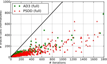
clearly outperforms the binarization variant. Notice that since AD3 with the active set method involves more computation per iteration, we plot the objective values with respect to the normalized number of oracle calls (which matches the number of iterations for the other methods).
7.2 Protein Design
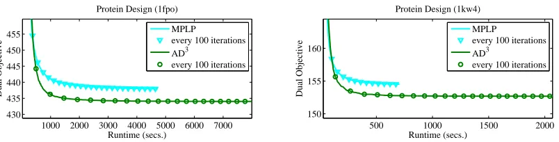
We compare AD3with the MPLP implementation8of Sontag et al. (2008) in the benchmark
protein design problems9 of Yanover et al. (2006). In these problems, the input is a three-dimensional shape, and the goal is to find the most stable sequence of amino acids in that shape. The problems can be represented as pairwise factor graphs, whose variables correspond to the identity of amino acids and rotamer configurations, thus having hundreds of possible states. Figure 6 plots the evolution of the dual objective over runtime, for two of the largest problem instances, i.e., those with 3167 (1fbo) and 1163 (1kw4) factors. These plots are representative of the typical performance obtained in other instances. In both cases, MPLP steeply decreases the objective at early iterations, but then reaches a plateau
8. Available at http://cs.nyu.edu/~dsontag/code; that code includes a “tightening” procedure for re-trieving the exact MAP, which we don’t use, since we are interested in the LP-MAP relaxation (which is what AD3 addresses).
Figure 5: Evolution of the dual objective in the experiments with random 20×20 Potts models with 8-valued nodes, generated as described in the main text. For PSDD and the accelerated dual decomposition algorithm, we chose η0 and as before.
For AD3, we set η = 1.0 in both settings (active set and binarization). In the active set method, no caching was used and the plotted number of iterations is corrected to make it comparable with the remaining algorithms, since each outer iteration of AD3 requires several calls to a MAP oracle (we plot the normalized number of oracle calls instead). Yet, due to warm-starting, the average number of inner iterations is only 1.04, making the active set method extremely efficient. For all methods, the markers represent every 100 iterations.
with no further significant improvement. AD3rapidly surpasses MPLP in obtaining a better dual objective. Finally, observe that although earlier iterations of AD3 take longer than those of MPLP, this cost is amortized in later iterations, by warm-starting the active set method.
1000 2000 3000 4000 5000 6000 7000 430
435 440 445 450 455
Runtime (secs.)
Dual Objective
Protein Design (1fpo)
MPLP
every 100 iterations AD3
every 100 iterations
500 1000 1500 2000 150
155 160
Protein Design (1kw4)
Runtime (secs.)
Dual Objective
MPLP
every 100 iterations AD3
every 100 iterations
200 400 600 800 1000 25.8
25.9 26 26.1
Number of Iterations
Dual
Objective
Frame−Semantic Parsing
0 200 400 600 800
42.12 42.14 42.16 42.18
100 200 300 400 500 20.1
20.2 20.3 20.4
200 400 600 800 1000 60.6
60.8 61 61.2 61.4
200 400 600 800 1000 63
64 65
66 MPLP
Subgrad.
AD3
Figure 7: Experiments in five frame-semantic parsing problems (Das, 2012, Section 5.5). The projected subgradient uses ηt = η0/t, with η0 = 1.0 (found to be the best
choice for all examples). In AD3,ηis adjusted as proposed by Boyd et al. (2011), initialized atη= 1.0.
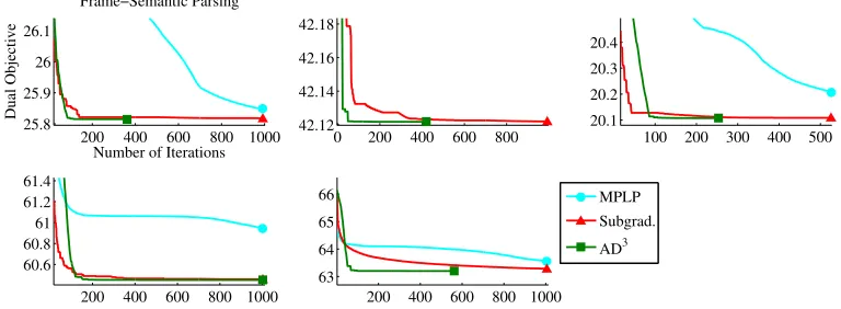
7.3 Frame-Semantic Parsing
We now report experiments on a natural language processing task involving logic con-straints: frame-semantic parsing, using the FrameNet lexicon (Fillmore, 1976). The goal is to predict the set of arguments and roles for a predicate word in a sentence, while re-specting several constraints about the frames that can be evoked. The resulting graphical models are binary constrained factor graphs with FOL constraints (see Das et al. 2012 for details about this task). Figure 7 shows the results of AD3, MPLP, and PSDD on the five most difficult problems (which have between 321 and 884 variables, and between 32 and 59 factors), the ones in which the LP relaxation is not tight. Unlike MPLP and PSDD, which did not converge after 1000 iterations, AD3 achieves convergence in a few hundreds of iter-ations for all but one example. Since these examples have a fractional LP-MAP solution, we applied the branch-and-bound procedure described in Section 4.5 to obtain the exact MAP for these examples. The whole data set contains 4,462 instances, which were parsed by this exact variant of the AD3 algorithm in only 4.78 seconds, against 43.12 seconds of CPLEX, a state-of-the-art commercial ILP solver.
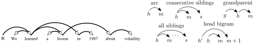
7.4 Dependency Parsing