A Reduced-Order Extrapolating Finite Difference Iterative Scheme for 2D Generalized Nonlinear Sine-Gordon Equation

http://www.sciencepublishinggroup.com/j/acm doi: 10.11648/j.acm.20180701.13

ISSN: 2328-5605 (Print); ISSN: 2328-5613 (Online)

A Reduced-Order Extrapolating Finite Difference Iterative

Scheme for 2D Generalized Nonlinear Sine-Gordon

Equation

Hong Xia

1

, Fei Teng

1

, Zhendong Luo

2, *

1_{School of Control and Computer Engineering, North China Electric Power University, Beijing, China} 2

School of Mathematics and Physics, North China Electric Power University, Beijing, China

Email address:

*

Corresponding author

To cite this article:

Hong Xia, Fei Teng, Zhendong Luo. A Reduced-Order Extrapolating Finite Difference Iterative Scheme for 2D Generalized Nonlinear Sine-Gordon Equation. Applied and Computational Mathematics. Vol. 7, No. 1, 2018, pp. 19-25. doi: 10.11648/j.acm.20180701.13

Received: December 17, 2017; Accepted: January 2, 2018; Published: January 18, 2018

Abstract:

In this study, a reduced-order extrapolating finite difference iterative (ROEFDI) scheme holding sufficiently high accuracy but containing very few degrees of freedom for the two-dimensional (2D) generalized nonlinear Sine-Gordon equation is built via the proper orthogonal decomposition. The stability and convergence of the ROEFDI solutions are analyzed. And the feasibility and effectiveness of the ROEFDI scheme are verified by numerical simulations. This means that the ROEFDI scheme is effective and feasible for finding the numerical solutions of the 2D generalized nonlinear Sine-Gordon equation.

Keywords:

Reduced-Order Finite Difference Scheme, Degree of Freedom, Generalized Nonlinear Sine-Gordon Equation, Proper Orthogonal Decomposition

1. Introduction

The Sine-Gordon equation is a nonlinear hyperbolic partial differential equation due to it including the d'Alembert operator and the sine of the unknown function. It was first presented by Bour in the research of surfaces of constant negative curvature in 1862 such as the Gauss

-Codazzi equation for surfaces of curvature (see [1]) and redeveloped by Frenkel and Kontorova in the research of crystal dislocations in 1939 (see [2]). This equation has attracted a lot of attention since 1970 because of the presence of soliton solutions. In addition, the nonlinear Sine-Gordon equation has also extremely vital applications in the field of nonlinear physics and is broadly used to depict lots of physical rules such as the telegraph line voltage variation and the collision of solitary wave (see, e.g., [3-6]).

Because the Sine-Gordon equation includes a nonlinear term about the sine of the unknown function and its known data and computational domain are usually very complex, it has generally no analytical solution. One has to rely on

numerical solutions. The finite difference (FD) scheme (see [6]) is one of the most valid numerical methods to solve the tow-dimensional (2D) nonlinear Sine-Gordon equation. However, the classical FD scheme for the 2D nonlinear Sine-Gordon equation is a macroscale system of equations including lots of unknowns so as to undertake very large calculating load in the real-life applications. Therefore, a vital problem is to lessen the unknowns (i.e., degrees of freedom) of the classical FD scheme so that it can save the computing time but its numerical solutions keeps sufficiently high accuracy.

reduced-order numerical methods (such as the POD-based reduced-order FD schemes and finite element and finite volume element methods as well as Galerkin spectral methods) have been widely applied in the numerical computations for PDEs (see, e.g., [12-21]). But, most existing reduced-order models as mentioned above were established via the POD basis of the classical numerical solutions at all time nodes, before recalculating the reduced-order numerical solutions at the same time nodes, which are some worthless repeated computations. Since 2013, some reduced-order extrapolating approaches based on POD technique for PDEs have been proposed successively in Luo's articles [22-25] in order to avoid the meaningless repeated computations.

As far as we know, there exists not any report that the POD method is utilized to simplify the classical FD scheme for the 2D generalized nonlinear Sine-Gordon equation. Therefore, in this work, we extend the approaches in [22-25] to the 2D generalized nonlinear Sine-Gordon equation, employing the POD technique to build a reduced-order extrapolating finite difference iterative (ROEFDI) scheme containing very few unknowns but having high enough accuracy. Especially, we are going to analyze the stability and convergence of the ROEFDI solutions by theoretical analysis and verify the feasibility and effectiveness of the ROEFDI scheme via numerical simulations.

The major difference between the ROEFDI scheme and the POD-based existing reduced-order extrapolating approaches (see, e.g., [22-25]) consists in that the ROEFDI scheme here is implicit and unconditionally stable so that its theoretical analysis and numerical simulations need more technique than the existing those as mentioned above, which are conditionally stable explicit schemes. Especially, the ROEFDI scheme here only uses the classical FD solutions on the first very short time span to constitute the POD basis and build the ROEFDI scheme. Therefore, it not only holds the unconditionally stable merit of the implicit FD scheme, but also includes not repeated computation as References [22-25]. Hence, it is the development and improvement over the existing those as mentioned above.

The remainder of the article is arranged as follows. The classical FD scheme for the 2D generalized nonlinear Sine-Gordon equation is built in Section 2. The POD basis is constituted in Section 3. The ROEFDI scheme for the 2D Sine-Gordon equation is built via the POD basis and the stability and convergence of the ROEFDI solutions is analyzed in Section 4. Some numerical simulations are displayed to verify the feasibility and effectiveness of the ROEFDI scheme in Section 5. Finally, some main conclusions are summarized in Section 6.

2. Classical FD Scheme for 2D Nonlinear

Sine-Gordon Equation

As a matter of convenience and without loss of

universality, consider the following 2D nonlinear Sine-Gordon equation.

+ − ∆ + sin

= , , , ∈ Ω × 0, , , , = 0, , , ∈ !Ω × 0, ,

, , 0 = " , , , ∈ Ω, #,$," ₌

% , , , ∈ Ω,

(1)

whereΩ = *, + × *, + ⊂ -._{is the bounded open set with}

the boundary !Ω, , , is an unknown function, and d

as well as are three known positive parameters, and

, , and _" , as well as _% , are three given functions.

The existence and uniqueness of the solution of the equation (1) have been provided in [6].

In order to make a rectangular net cutting Ω/ × 00, 1 =

0*, +1._{× 00, 1, let N and M be two positive integers, h=(b} -a)/N denote the spatial step and 2=T/M be the time step. Thus, we can get ₃= * + 4ℎ, ₆= * + 7ℎ 4, 7 =

1, 2, … , ; − 1 , and _<= =2 = = 1, 2, … , > . Define

36

< _̅= 3,6<A%− 2 3,6< + 3,6<B%

2. ,

36

< _C= 3,6<A%− 3,6<B%

22 ,

36 <

##̅= 3A%,6 < _{− 2}

36 < ₊

3B%,6 <

ℎ. ,

36 <

$$D= 3,6A% < _{− 2}

36 < ₊

3,6B% <

ℎ. .

The implicit FD scheme of the equation (1) is as follows.

36 < _̅+

36< C− 0 36<A% ##̅+ E 36<A%1$$DF

+ sinE 36<G = 3,6<, (2)

3,6" = "E 3, 6G, 3,6% − 3,6B%= 22 %E 3, 6G. (3)

Thus, by simplifying (2) and (3), we obtain

− H._E 3B%,6 <A% ₊

3A%,6 <A% ₊

3,6B%<A% + 3,6A%<A%G + 1 + 0.5 2 + 4 H.

3,6<A%

= 0.5 2 − 1 3,6<B%+ 2 3,6< − 2. sinE 3,6<G + 2. 3,6<, (4)

36 " ₌

",3,6, 3,6B%= 3,6% − 22 %,3,6, (5)

where _",3,6= _"E ₃, ₆G, _%,3,6= _%E ₃, ₆G, H = 2/ℎ is net ratio. By taking = = 0 in (4) and using (5), we obtain

− H._E 3B%,6

% ₊

3A%,6

% ₊

3,6B%

% ₊

3,6A%

% _{G + 2 + 4 H}. 3,6

% ₌

22 1 − 0.5 2 %,3,6+ 2 ",3,6− 2. sinE ",3,6G + 2. 3,6". (6)

L<₌ %,% < _,

.,% < _{, … ,}

MB%,% < _,

%,. < _,

.,. < _{, …,}

MB%,. < _{, … ,}

%,MB%< , .,MB%< , … , MB%,MB%< N O<₌

%,%<, .,%<, … , MB%,%< , %,.<, .,.<, … , MB%,.< , …,

%,MB%< , .,MB%< , … , MB%,MB%< N, P L< _{= sin %,%}< _{, sin}

.,%

< _{, … , sin} MB%,% < _,

sin %,.< , sin .,.< , … , sin MB%,.< , sin %,MB%< , sin .,MB%< , … , sin MB%,MB%< N,

L%= % %, % , % ., % , … , % MB%, % , % %, . ,

% ., . , … , % MB%, . , … , % %, MB% ,

% ., MB% , … , % MB%, MB% N,

L"= " %, % , " ., % , … , " MB%, % , " %, . ,

" ., . , … , " MB%, . , … , " %, MB% ,

" ., MB% , … , " MB%, MB% N,

Q =

R S S T

−2 1 0

1 −2 1

0 1 −2

⋯ 0 0 ⋯ 0 0 ⋱ 0 0 ⋮ ⋮ ⋱

0 0 0 0 0 0

⋱ ⋱ ⋮

⋱ −2 1 ⋯ 1 −2X

Y Y Z ,

[ =

R S S S

T−2 ⋯\

M ]^_`a 1

⋮ −2 ⋱

1 ⋱ −2

0 ⋯ 0 ⋱ ⋱ ⋮ ⋱ ⋱ 0 0 ⋱ ⋱

⋮ 0 ⋱ 0 0 0

⋱ ⋱ 1

⋱ −2 ⋮

1 ⋯b

M ]^_`a −2X Y Y Y Z .

Then, the matrix forms of (4) and (6) are as follows.

cL<A%

= 0.5 2 − 1 L<B%_{+ 2L}<_{− 2}. _{P L}< _{+ 2}._O<_{, (7)} c%d%= L%+ 2L"− 2. P L" + 2.O", (8) where = = 1,2, … , ; − 1, c = 1 + 0.5 2 e + H. Q + [ ,

c%= 2e + H. Q + [ , and I is the unit matrix.

Define the norm of matrix cf by g cfg_.,.= sup_#j"g cfkg_./

‖ k‖., where ‖ k‖_. denotes the norm of vector x. The classical FD scheme (7) and (8) has the following results.

Theorem 1. If ∈ mn 0, 1; p_"% Ω ∩ p. Ω is the exact solution for the 2D nonlinear Sine-Gordon equation, then the classical FD scheme (7) and (8) has a unique set of solutions

rL<_s<t%u _{, which is conditionally stable and has the following}

error estimates

gLf<_{− L}<_g

.= v ℎ., 2. , = = 1,2, … , >, (9)

where Lf<= _%, _%, _< , _., _%, _< , … , _MB%, _%, _< ,

E %, .,, <G, ., ., < , … , MB%, ., < , … , %, MB%, < , ., MB%, < , … , MB%, MB%, < N are formed by

the exact solution

Proof. It is easily known that the matrices w and w_% both are positive definite. Therefore, the classical FD scheme (7) and (8) has a unique set of solutions rd<s_<t%u .

By the properties of the matrix norm (see, e.g., [26]), we have ‖ cB%‖_.,.≤ 1 + 0.5 2 B% and ‖ c_%B%‖_.,.≤ 1/2. Because ‖ P L< ‖_.≤ ‖ L<‖_., when 2 is sufficiently small, from (8) and (7), we have

‖L%_‖.≤%

.0‖L%‖.+ 2 + 2. ‖L"‖.+ 2.‖O"‖.1, (10) ‖L<A%_‖

.≤1 − 0.5 2_{1 + 0.5 2 ‖L}<B%‖.+_{1 + 0.5 2 ‖L}2 <‖.

+_{1 + 0.5 2 ‖P L}2. < _‖

.+ 2

.

1 + 0.5 2 ‖O<‖.

≤ ‖L<_‖

.+1 − 0.5 2_{1 + 0.5 2 ‖L}<B%‖.+ ‖L<‖.

+_%A".{|yy z ‖L<_‖.+ y uf}

%A".{|y, (11)

where = = 1,2, … , > − 1, and >f_€= max_%ƒ<ƒu‖O<‖_.. By summing (11) from 1 to = − 1, we have

‖L<_{‖.≤ >"+} >2.>f€

1 + 0.5 2 +2 − 2 + 2 .

1 + 0.5 2 „gL3g. <B%

3t" ,

= = 1,2, … , >, (12) where >_"= 0‖L_%‖_.+ 2 + 2. ‖L"‖_.+ 2.‖O"‖_.1/2.

By using Gronwall’s inequality (see, e.g., [7, 26]), from (12), we have

‖d<_‖

.≤ …>"+_%A".{|yuy uf}† exp ….B|yAy z_%A".{|y †, (13) where = = 1,2, … , >. Thus, when 00, T1 is the finite time span, > = /2 is a finite integer so that the set of FD solutions rL<s_<t%u are bounded. Therefore, by Lax’s stability theorem (see, e.g., [7, 26]), we easily deduce that the FD solutions rL<s_<t%u are unconditionally stable. By Taylor’s formulas or the procedure of (2), we easily deduce the error estimates (9), which completes the proof of Theorem 1.

If , , , _" , , _% , , 2, ℎ, and parameters

and as well as d are given, then we can get a set of FD solutionsrd<s_<t"u by solving (7) and (8). A subset rL<s_<t"ˆ (usually ‰ ≪ >), called as the snapshots, is extracted from the first ‰ solution vectors ofrL<s_<t"u .

Remark 1. In this work, we adopt a simpler linearizing implicit FD scheme to discrete the 2D nonlinear Sine-Gordon equation, but the ideas and approaches here can be easily extended other FD schemes, for example, staggered direction FD scheme.

3. Constitution of POD Basis

c = L …‹_{Œ Œ† •}Œ N_,

where L = EŽ_%, Ž_., … , Ž_MB% G ∈ -MB% × MB% , and

• = •%, •., … , •ˆA% ∈ -ˆA% × ˆA% are, separately, two orthogonal matrices consisting of the orthonormal eigenvectors of the c cN and cNc ,

‹ = diag ‘%, ‘., … , ‘’ ∈ -’×’ is the diagonal matrix

associated with c , and ‘₆> 0 (7 = 1,2, … , H =rank(c ) are the positive singular values arranged decreasingly. The relationship between the positive singular values of the matric c with the positive eigenvalues of the matric c cN is ”₆= ‘₆ (7 = 1,2, … , H).

Because the number of mesh nodes ; − 1 . is much greater than the number of the snapshots ‰ + 1 , so the order ; − 1 . of matrix c_•cN is much greater than the order ‰ + 1 of matrix cNc , but their nonzero eigenvalues are identical. Thus, we firstly find out the eigenvectors

•– 4 = 1,2, … , H of cNc , then we immediately obtain

H H ≤ ‰ + 1 eigenvectors associated with the nonzero eigenvalues for matrix c cN via the formula Ž₃= c •₃/

”3 4 = 1,2, … , H .

Let c_u— = ∑ ‘u_6t%— ₆Ž₆•₆N, where ‘₆ (7 = 1,2, … , > ) are the first > singular values of matrix ™ , Ž₆ and •₆ (7 =

1,2, … , > ) are the first > eigenvectors of matrices d and

š , separately. If > < H =rank (c , by means of the relationship between the spectral radius with the matrix norm, we obtain the next formula (see, e.g., [17])

min_{_œ•ž Ÿ ƒu}

—gc − Qfg.，.= gc − cu—g.,.

= ‖c − ¡¡N_{c ‖}

.,.= ‘u—A%, (14)

where ¡ = Ž_%, Ž_., … , Ž_u— . Write

L¢<= ¢,%,%< , ¢,.,%< , … , ¢,MB%,%< , ¢,%,.< , ¢,.,.< , … , ¢.MB%,.< , … , %,MB%< , .,MB%< , … , MB%,MB%< N = = 1,2, … , ‰ + 1

as the ‰ + 1 column vectors of matrix c_u— and £_< = =

1,2, … , ‰ + 1 as the unit vectors with n-th component being 1. Then, by means of the norm properties for vectors and matrices, we obtain

‖L<_{− L} ¢ <_‖

.= ‖L<− ¡¡NL<‖.= g c − cu— £<g_.

≤ gc − cu—g_.,.‖ £<‖.= ‘u—A%, (15)

where = = 1,2, … , ‰ + 1. The formula (15) implies that

L¢<= ¡¡NL< is the optimum approximation to L<. We

deduce from (14) and (15) that ¡ = Ž_%, Ž_., … , Ž_u— is a set of optimal basis, which is called as a series of POD basis.

4. ROEFDI Scheme for 2D Sine-Gordon

Equation

If the ROEFDI solutions are still denoted byL_¢< =

¢,%,% < _,

¢,.,% < _{, … ,}

¢,MB%,% < _,

¢,%,. < _,

¢,.,. < _{, … ,}

¢.MB%,. < _{, … ,}

%,MB%< , .,MB%

< _{, … ,}

MB%,MB%

< N _{= = 1,2, … , ‰ + 1, … , > and put} ¤< _{= E}

%<, .<, . . , u<—G

N

= = 1,2, … , ‰ + 1, … , > , from the Section 3, we have gained the first ‰ ‰ ≤ > ROEFDI solutions L_¢<= ¡¡NL<=: ¡¤< = = 1,2, … , ‰ . Thus, if the solution vectors L< = = ‰ + 1, ‰ + 2, … , > for the classical FD scheme (7) are approximated by L_¢<=

¡¤< _{= = ‰ + 1, ‰ + 2, … , > , i.e., L}< _{are replaced with} L¢<= ¡¤< = = ‰ + 1, ‰ + 2, … , > , we can obtain the

ROEFDI scheme based on the POD basis as follows.

¡¤<_{= ¡¡}N_L<_{, 1 ≤ = ≤ ‰;} c¡¤<A%_{= 0.5 2 − 1 ¡¤}<B%_{+ 2¡¤}<

−2. _{P ¡¤}< _{+ 2}._O<_{, ‰ ≤ = ≤ > − 1,} L¢<= ¡¤<, 1 ≤ = ≤ >,

(16)

where L< 1 ≤ = ≤ ‰ are the known classical FD solution vectors of (7). The ROEFDI scheme (16) is simplified as

follows.

¤<_{= ¡}N_L<_{, 1 ≤ = ≤ ‰;} ¡N_c¡¤<A%_{= 0.5 2 − 1 ¤}<B%_{+ 2¤}< −2. _¡N_{P ¡¤}< _{+ 2}._¡N_O<_{, ‰ ≤ = ≤ > − 1,}

L¢<= ¡¤<, 1 ≤ = ≤ >.

(17)

The system of equations (16) or (17) is called as the ROEFDI scheme. Because the FD scheme (7) includes

; − 1 . _{unknowns at each time node, whereas the ROEFDI}

scheme (17) at the same node only includes > unknowns and > ≪ ; − 1 2. Therefore, we can clearly realize the advantage of the ROEFDI scheme (17).

There are the following main results of the existence, stability, and convergence of the ROEFDI solutions for the ROEFDI scheme (17).

Theorem 2. Under the conditions of Theorem 1, the ROEFDI scheme (17) has a unique set of solutions rL_¢<s_<t%u , which is unconditionally stable and has the following error estimates:

‖L<_{− L} ¢ <_‖

.≤ ¦_{¨ = §”}§”u—A%, 1 ≤ = ≤ ‰, u—A%, ‰ + 1 ≤ = ≤ >,

(18)

where L< 1 ≤ = ≤ ; are the classical FD solution vectors of (7) and ¨ = =_%A".{|y. exp © = − ‰ ….B|yAy z_%A".{|y †ª. Further, the ROEFDI solutions rL=s₌₌₁> have the following error estimates:

gLf<_{− L} ¢ <_g

. =

= ´ vEℎ., 2., §”u—A%G, 1 ≤ = ≤ ‰，

vEℎ._{, 2}._{, ¨ = §”u}

—A%G, ‰ + 1 ≤ = ≤ >,

(19)

exact solution.

Proof. By using L_¢<= ¡¤= = = 1, 2, … , > , the ROEFDI scheme (16) is reverted into the following form

L¢<= ¡¡Nd<, 1 ≤ = ≤ ‰; (20) cL¢<A%= 0.5 2 − 1 L¢<B%+ 2L¢<

−2. _{P L} ¢

< _{+ 2}._O<_{, ‰ ≤ = ≤ > − 1. (21)}

Because the classical FD solutions L< = = 1, 2, … , > are known and bounded, when = = 1, 2, … , ‰, from (20), we obtain unique solutions L_¢<= ¡¡NL< = = 1, 2, … , ‰ . Moreover, when = = ‰ + 1, ‰ + 2, … , >, by using the same approaches as proving Theorem 1, we easily prove that the ROEFDI scheme (21) has a unique set of solutions rL_¢<s_<tˆA%u and the ROEFDI solutions

rL¢<s<tˆA%u are unconditionally bounded. Therefore, the

ROEFDI scheme (17) has a unique set of solutions

rL¢<s<t%u and, by Lax’s stability theorem (see, e.g.,

[7,26]), it is concluded that the ROEFDI solutions

rL¢<s<t%u are unconditionally stable.

When = = 1,2, … , ‰, from (15), we immediately obtain the following error estimates

‖L<_{− L} ¢ <_‖

.= ‖L<− ¡¡NL<‖.≤ §”u—A%, (22)

where = = 1,2, … , ‰.

Let µ<= L<− L_¢<. By Lagrange’s mean value theorem, we have ‖P L< − P L_¢< ‖_.≤ ‖L<− L_¢<‖_.≤ ‖µ<‖_.. Because ‖ wB%‖_.,.≤ 1 + 0.5 2 B%, when = = ‰ + 1, ‰ +

2, … , >, from (7) and (21), we have

‖µ<A%_{‖.≤ ‖ 0.5 2 − 1 c}B%_µ<B%_{+ 2c}B%_µ<_‖. + ‖2. _{0P L}< _{− ¶ L}

¢ < _1‖

.

≤ ‖µ<_‖.+1 − 0.5 2

1 + 0.5 2 ‖µ<B%‖.+ ‖µ<‖.

+_%A".{|yy z ‖µ<_{‖.. (23)}

By summing (23) from ‰ to = − 1 and using (22) and the Gronwall inequality (see, e.g., [7, 26]), we have

‖µ<_‖.≤ 2

1 + 0.5 2 ·”u—A%+

2 − 2 + 2.

1 + 0.5 2 „gµ3g. <B%

3tˆ

≤ ¨ = §”u—A%, ‰ + 1 ≤ = ≤ >. (24)

Combining (22) with (24) yields (18). Combining Theorem 1 with (18) yields (19). Thus, we accomplish the proof of Theorem 2.

Remark 2. The error factors §”_u—A% and ¨ = =

.

%A".{|yexp © = − ‰ …

.B|yAy z

%A".{|y †ª in Theorem 2 are caused for

reducing order of the classical FD scheme and for the extrapolating iteration, respectively. They can be used as the suggestions that one chooses the number > of POD bases and renew the POD bases in actual computing such that the ROEFDI solutions achieve the desirable accuracy.

5. Numerical Experiments

In the equation (1), we take

" , = 1 − cos ¹ 1 − cos ¹ ,

% , = cos ¹ − 1 1 − cos ¹ ,

, , = −¹. _{cos ¹ + cos ¹}

−2 cos ¹ cos ¹ exp −

+2 sin0 1 − cos ¹ 1 − cos ¹ exp − 1.

Thus, an analytical solution , , = 1 −

cos ¹ 1 − cos ¹ exp − for equation (1) can been obtained.

Consider the numerical simulations in Ω/ = 00, 21 × 00, 21. Denote the analytical solution matrix by

•º = Lf%_{, Lf}._{, … , Lf}u _{, the classical FD solution matrix by} •%= L%, L., … , Lu , and the ROEFDI solution matrix with the POD basis generating by the first ‰ rows in _% by

•.= L¢%, L¢., … , L¢u . Write » •º, •¼ = ‖•º − •¼‖.,. ½ = 1,2 . Denote the operating time of the classical FD and the ROEFDI scheme by _% ¾ and _. ¾ , respectively. When

2 = 0.05 and ℎ = 1/20, Table 1 exhibits the errors between the analytical solution •º and the ROEFDI solutions •_. with varying number > of the POD basis.

Table 1. The errors between the accurate solution with the ROEFDI solutions at T=10.

¿• 1 3 5 7

» •º, •. 8.6406 × 10B 6.6028 × 10B 6.6823 × 10B 6.5968 × 10BÂ

By reckoning, we have obtained that the error between the analytical solution and the classical FD solution at = 10 is

» •º, •% = 6.6034 × 10BÂ. Thus, Table 1 reveals that the error between the errors between the analytical solution and the

ROEFDI solutions with varying numbers > of POD basis closes very to the analytical solution and the FD solution at =

10.

Table 2. The errors between classical FD solutions and ROEFDI solutions as well as operating time at T=10.

¿• 1 3 5 7

» •%, •. 4.1559 × 10BÂ 5.6413 × 10B{ 2.1558 × 10B{ 1.6365 × 10B{

. ¾ 19.69l 21.41 23.14 24.41

Table 2 exhibits the errors between the classical FD solution matrix •_% and the ROEFDI solution matrix •_. as well as their implementing time with varying numbers > of

POD basis.

that the implementing time _. ¾ ≤24.41s seeking the ROEFDI solution is far fewer than that finding the classical FD solution % ¾ =107.18s).

Tables 1 and 2 reveal also that the numerical errors correspond with the theoretical errors because the errors between the analytical solution and the classical FD one and between the analytical solution and the ROEFDI one have been very small, but the errors between the classical FD solution and the ROEFDI one is smaller and the implementing time of the ROEFDID solution is fewer than that of the classical one. Therefore, the ROEFDI scheme is high-efficiency and reliable for the 2D nonlinear Sine-Gordon equation and alleviates greatly computing load.

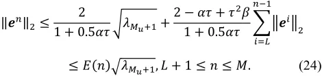
Figure 1. The classical FD solution at t=10.

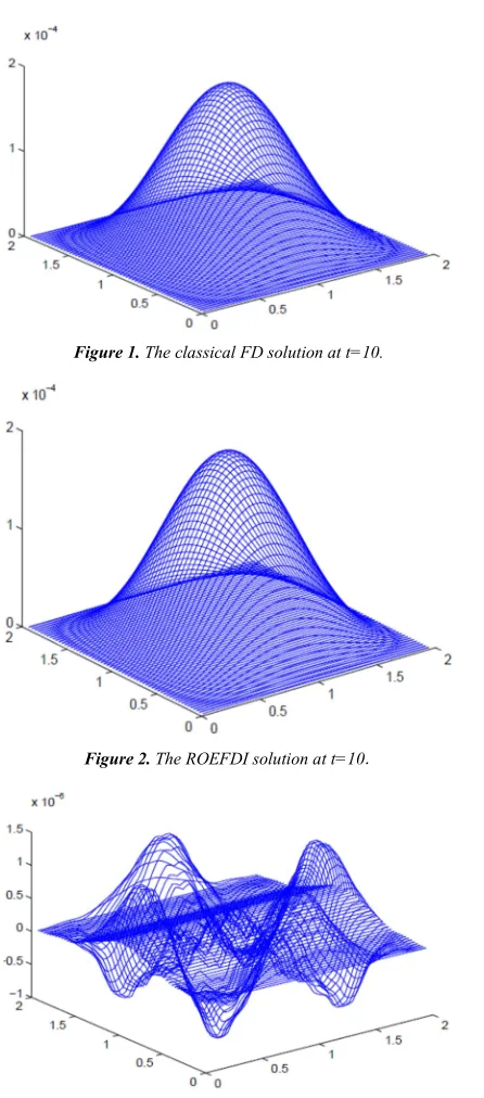
Figure 2. The ROEFDI solution at t=10.

Figure 3. The error between the classical FD solution and the ROEFDI solution at t=10.

When 2 0.05, 5 1/20, 10, > 3, the classical FD solution and the ROEFDI one as well as the error between them are depicted graphically in Figures 1 and 2 as well as 3 at 10, respectively. Figures 1 and 2 exhibit quasi-identical similarity. However, the ROEFDI solution is better than the classical FD one due to using more initial data, i.e., three POD bases and containing very unknowns as well as lessening the truncated error accumulation. Figure 3 shows that the error between the classical FD solution with the ROEFDI solution is very small, but the implementing time seeking the ROEFDI solution has been greatly lessened.

6. Conclusions

In this article, the ROEFDI scheme for the 2D generalized nonlinear Sine-Gordon equation has been built by means of the POD technique. First, the ensemble of date is extracted from the first few FD solutions for the 2D nonlinear Sine-Gordon equation. And then, the POD basis of the ensemble is formulated by means of the POD technique and the ROEFDI scheme having sufficiently high accuracy but containing very few unknowns is built by replacing the unknowns of FD scheme with the linear-combination of the POD bases. Finally, the stability and convergence of the ROEFDI solutions are analyzed. The numerical simulations have expressed that the numerical errors between the classical FD solutions and the ROEFDI ones correspond with the theoretical results. This implies that the ROEFDI scheme is high-efficiency and reliable for solving the 2D nonlinear Sine-Gordon equation.

Although we restrict our technique to the 2D nonlinear Sine-Gordon equation on the domain Ω/=[a, b] [a, b], our approach can extend to the more general domains, even extend to the more complicated engineering problems. Therefore, our technique has important applied prospect.

Acknowledgements

This work is jointly supported by the National Science Foundation of China (11671106) and the Fundamental Research Funds for the Central Universities (2017XS067).

References

[1] E. Bour, “Théorie de la déformation des surfaces,” J. Ecole Imperiale Polytechnique, 1862, 19, 1–48.

[2] J. Frenkel and T. Kontorova, “On the theory of plastic deformation and twinning,” Izvestiya Akademii Nauk SSSR, Seriya Fizicheskaya, 1939, 1 (3), 1607–1614.

[3] A. E. Koshelev, “Stability of dynamic coherent states in intrinsic Josephson-junction stacks near internal cavity resonance,” Phys. Rev., 2010, 82, 174512–174526.

[5] H. Jafari, R. Soltani and C. M. Khalique, “Exact solutions of two nonlinear partial differential equations by using the first integral method,” Boundary Value Problems, 2013, 2013 (1), 1–9.

[6] S. F. Zhou, “Dimension of the global attractor for the damped Sine-Gordon equation,” Acta Mathematica sinica, 1996, 39 (5), 597–601.

[7] T. Chung, “Computational Fluid Dynamics”, Cambridge University Press, Cambridge, 2002.

[8] L. Sirovich, “Turbulence, the dynamics of coherent structures: part I-III,” Quart. Appl. Math., 1987, 45, 561–590.

[9] J. S. Hesthaven, G. Rozza and B. Stamm, “Certified Reduced Basis Methods for Parametrized Partial Differential Equations,” Springer International Publishing, 2016.

[10] H. Xia and Z. D. Luo, “A stabilized MFE reduced-order extrapolation model based on POD for the 2D unsteady conduction-convection problem,” Journal of Inequalities and Applications, 2017, 2017 (124), 1–17.

[11] P. Benner， A. Cohen, M. Ohlberger and A. K. Willcox, “Model Reduction and Approximation: Theory and Algorithm,” Computational Science & Engineering, SIAM, 2017.

[12] A. Quarteroni, A. Manzoni and F. Negri, “Reduced Basis Methods for Partial Differential Equations,” Springer International Publishing, 2016.

[13] Z. D. Luo and S. J. Jin, “A reduced-order extrapolation spectral-collocation scheme based on POD method for 2D second-order hyperbolic equations,” Mathematical Modelling and Analysis，2017, 22 (5), 569–586.

[14] Z. D. Luo, F. Teng and J. Chen, “A POD-based reduced-order Crank-Nicolson finite volume element extrapolating algorithm for 2D Sobolev equations,” Mathematics and Computers in Simulation, 2018，146, 118–133.

[15] Z. D. Luo and F. Teng, “An optimized SPDMFE extrapolation approach based on the POD technique for 2D viscoelastic wave equation,” Boundary Value Problems, 2017, 2017 (6), 1–20.

[16] Z. D. Luo and F. Teng, “Reduced-order proper orthogonal decomposition extrapolating finite volume element format for

two-dimensional hyperbolic equations,” Applied Mathematics and Mechanics, 2017, 38 (2), 289–310.

[17] Z. D. Luo, “A POD-based reduced-order TSCFE extrapolation iterative format for two-dimensional heat equations,” Boundary Value Problems, 2015, 2015 (59), 1–15.

[18] Z. D. Luo, “A reduced–order SMFVE extrapolation algorithm based on POD technique and CN method for the non– stationary Navier–Stokes equations,” Discrete and Continuous Dynamical Systems Series B, 2015, 20 (4), 1189–1212. [19] Z. D. Luo, “Proper orthogonal decomposition-based

reduced-order stabilized mixed finite volume element extrapolating model for the nonstationary incompressible Boussinesq equations,” Journal of Mathematical Analysis and Applications, 2015, 425 (1), 259–280.

[20] R. Stefanescu, A. Sandu and I. M. Navon, “Comparison of POD reduced order strategies for the nonlinear 2D shallow water equations,” International Journal for Numerical Methods in Fluids, 2014, 76 (8), 497–521.

[21] G. Dimitriu, R. Stefanescu and I. M. Navon, “POD-DEIM approach on dimension reduction of a multi-specices host-parasition system,” Ann. Acad. Rom. Sci. Ser. Math. Appl., 2015, 7 (1), 173–188.

[22] Z. D. Luo, “A POD-based reduced-order finite difference extrapolating model for the non-stationary incompressible Boussinesq equations,” Adv. Difference Eq., 2014, 2014 (272), 1–18.

[23] Z. D. Luo, S. J. Jin and J. Chen, “A reduced-order extrapolation central difference scheme based on POD for two dimensional fourth-order hyperbolic equations,” Appl. Math. Comput., 2016, 289, 396–408.

[24] Z. D. Luo, “A POD-based reduced-order TSCFE extrapolation iterative format for two-dimensional heat equations,” Bound. Value Probl., 2015, 59 (1), 1–15.

[25] J. An, Z. D. Luo, H. Li and P. Sun, “Reduced-order extrapolation spectral-finite difference scheme based on POD method and error estimation for three-dimensional parabolic equation,” Front. Math. China, 2015, 10 (5), 1025–1040. [26] W. S. Zhang, “Finite Difference Methods for Partial