Extensions to Metric Based Model Selection

Extensions to Metric-Based Model Selection

Yoshua Bengio [email protected]

Nicolas Chapados [email protected]

Dept. IRO, Université de Montréal

C.P. 6128, Montreal, Québec, H3C 3J7, Canada

Editors: Isabelle Guyon and André Elisseeff

Abstract

Metric-based methods have recently been introduced for model selection and regularization, often yielding very significant improvements over the alternatives tried (including cross-validation). All these methods require unlabeled data over which to compare functions and detect gross differences in behavior away from the training points. We introduce three new extensions of the metric model selection methods and apply them to feature selection. The first extension takes advantage of the particular case of time-series data in which the task involves prediction with a horizon h. The idea is to use at t the h unlabeled examples that precede t for model selection. The second extension takes advantage of the different error distributions of validation and the metric methods: cross-validation tends to have a larger variance and is unbiased. A hybrid combining the two model selection methods is rarely beaten by any of the two methods. The third extension deals with the case when unlabeled data is not available at all, using an estimated input density. Experiments are described to study these extensions in the context of capacity control and feature subset selection.

Keywords: Metric-based Methods, Model Selection

1. Model Selection and Regularization

Supervised learning algorithms take a finite set of input/output training pairs {(x1,y1), ...,

(xm,ym)}, sampled (usually independently) from an unknown joint distribution P(X,Y), and at-tempt to infer a function g∈

G

the generalization error). In many cases one faces the dilemma that if

G

occurs if the dimension of X is too large, then the average training set loss (training error) will

be low but the expected loss may be large (overfitting), and vice-versa if

G

(underfitting).

In many cases one can define a collection of increasingly complex function classes

G0

G1

··· ⊂

G

selection methods attempt to choose one of these function classes to avoid both overfitting and

underfitting. Variable subset selection is a form of model selection in which one has to select both the number of input variables and the particular choice of these variables (but note that the two decisions may be profitably decoupled). One approach to model selection is based on complexity

penalization (Vapnik, 1982, 1998, Rissanen, 1986, Foster and George, 1994): one first applies the

learning algorithm to each of the function classes (on the whole training set), yielding a sequence of hypothesis functions g0,g1,.... Then one of them is chosen based on a criterion that combines

class

G

data: one estimates the generalization error by repeatedly training on a subset of the data and

testing on the rest (e.g. using the bootstrap, leave-one-out or K-fold cross-validation). One uses this generalization error estimator in order to choose the function class that appears to yield the lowest generalization error. Cross-validation estimators have been found to be very robust and difficult to beat (they estimate generalization error almost unbiasedly, but possibly with large variance). The

metric-based methods introduced by Schuurmans (1997) and Schuurmans and Southey (2002) are

somewhat in-between in that they take advantage of data not used for training in order to introduce a complexity penalty or a regularization term. These methods take advantage of unlabeled data: the behavior of functions corresponding to different choices of complexity are compared on the training data and on the unlabeled data, and differences in behavior that would indicate overfitting are exploited to perform model selection, regularization, or feature selection.

Regularization methods are a generalization of complexity penalization methods in which one

looks for a function in the larger class

G

the average training loss and a penalization for complexity, e.g., minimizing curvature (Poggio and Girosi, 1990). These approaches are not restricted to a discrete set of complexity classes and may potentially strike a better compromise between fitting the training data and avoiding overfitting.

An overview of advances in model selection and feature selection methods can be found in a recent Machine Learning special issue (Bengio and Schuurmans, 2002), and of course in the other papers of this special issue. This paper proposes new model selection methods and applies them to feature selection. The application to feature selection is based on forward stepwise selection to select the feature subsets (among features subsets of a given size) prior to applying the model selection (to select the number of features, i.e., the size of the subsets), as explained in Section 3.3.1 and in Algorithm 1. Model selection is represented by a functional S that takes a set of learning algorithms(A0,A1,...,An)along with a data set D as arguments, and returns an integer index i∗∈ {0,...,n}representing the selected model. In this setting, a “learning algorithm” is represented by a functional A that takes a data set D and returns a learned function. For example A could correspond to minimizing an empirical error over a fixed class of functions, while S could be one of the metric model selection methods.

This paper proposes extensions of previously-proposed metric-based model selection methods and applies them to feature selection problems. In Section 3 we present a first extension that takes advantage of the particular case of time-series data in which the task involves prediction over a given horizon. The idea is to use at t the unlabeled data that just precedes t but cannot be used for training. Experimental results on feature selection for auto-regressive data are reported in Section 3.3. For time-series data, a common feature selection problem is that of choosing the appropriate lags of the input time-series. Even though the series is one-dimensional, time-series prediction is a high-dimensional learning problem when there are long-term dependencies and one considers all the past values as potential inputs.

Algorithm 1 Stepwise Feature Subset Selection by Model Selection

Input: data set D, learning algorithm A, model selection algorithm S, loss functional L, and set of

input features F. Write V(A,FN) for the restriction of A that uses only the inputs features in the subset of N input features FN. Write Remp(A,D)for the training error when applying A on D, and

write i∗=S((A0,A1,...,An),D)the output of a model selection algorithm, which returns the index of one of the algorithms in(A0,A1,...,An)based on data D.

•Letn=|F|the number of input variables. •LetF0={}an initially empty set of features.

•LetA0=V(A,F0)the algorithm that does not use any input.

•ForN=1 to n

•Let f∗=argmin_f∈F\FN−1Remp(V(A,FN−1∪ {f}),D), the next best feature.

•LetFN=FN−1∪ {f∗}, the larger feature subset.

•LetAN=V(A,FN), the corresponding restricted algorithm. •Leti∗=S((A0,A1,...,An),D), the selected model index.

Output: the selected subset Fi∗ and the selected model Ai∗.

unlabeled data, one simply samples from an estimated input density (trained on the input part of the training data). Model selection experiments are performed on both artificial and real data sets using a Parzen windows to estimate the input density, and showing results often as good as when unlabeled data is available.

2. Metric-Based Model Selection and Regularization

Metric-based methods for model selection and regularization are based on the idea that solutions that overfit are likely to behave very differently on the training points and on other points sampled from the input density PX(x). This occurs because the learning algorithm tries to reduce the loss at the training points (but not necessarily elsewhere since no data is available there), whereas we want the solution to work well not only on the training points but in general where PX(x)is not small. These metric-based methods are all based on the definition of a metric (or pseudo-metric) on the space of functions, which allows to judge how far two functions are from each other:

d(f,g)def=ψ(E[L(f(X),g(X))])

where the expectation E[·]is over PX(x) andψis a normalization function. For example with the quadratic loss L(u,v) = (u−v)2, the proper normalization function isψ(z) =z1/2. Although PX(x) is unknown, Schuurmans (1997) proposed to estimate d(f,g)using an average dU(f,g)computed on an unlabeled set U (i.e., points xi sampled from PX(x)but for which no associated yi is given). In what follows we shall use dU(f,g)to denote the distance estimated on the unlabeled set U :

dU(f,g)

def

=ψ 1

|U|_i

∑

!

(1)

set T :

dT(f,g)def=ψ 1

|T|_i

∑

!

In addition, the following notation is introduced to compare a function to the “truth” (the conditional distribution PY|X):

d(g,PY|X)

def

=ψ(E[L(g(X),Y)])

and on a data set S:

dS(g,PY|X)

def

=ψ 1

|S|

∑

!

.

Schuurmans (1997) first introduced the idea of a metric-based model selection by taking advantage of possible violations of the triangle inequality, with the TRI model selection algorithm, which chooses the last hypothesis function gl (in a sequence g0,g1,...of increasingly complex functions)

that satisfies the triangle inequality dU(gk,gl)≤dT(gk,PY|X) +dT(gl,PY|X)with every preceding hypothesis gk, 0≤k<l. Improved results were described by Schuurmans and Southey (2002) with a new penalization model selection method, based on similar ideas, called ADJ, which chooses the

hypothesis function gl which minimizes the adjusted loss

ˆ

d(gl,PY|X)

def

=dT(gl,PY|X)max k<l

dU(gk,gl)

dT(gk,gl).

See Schuurmans and Southey (2002) for more detailed justification and for experiments showing that these two methods outperform classical model selection procedures (including cross-validation) on some small artificial data sets (with between 10 and 30 training examples) on which overfitting can be severe.

This idea of a metric-based method to control overfitting was extended to the regularization paradigm with the ADA algorithm, which in the case of regression is defined by the following regularized training criterion:

min

g∈GdT(g,PY|X)max

dU(g,φ)

dT(g,φ),

dT(g,φ)

dU(g,φ)

whereφis a kind of prior function which can be chosen for example as the constant average of the

yi’s. Even better results were obtained with this method, and comparisons were performed

(Schu-urmans and Southey, 2002) that show ADA not only to beat in most cases a wide array of model selection and regularization techniques, but also to often beat the oracle model selection method (that picks githat minimizes dU(gi,PY|X)out of a finite set). This may occur because ADA is a reg-ularization technique that can thus make a finer trade-off between overfitting and underfitting. Note however that our experiments suggest that ADA involves an optimization problem which can some-times be tricky and requires significantly more computation than the other metric model selection methods.

It is interesting to point out here that the metric model selection methods have something very important in common with Vicinal Risk Minimization (VRM) (Chapelle et al., 2001). Both seem to work by penalizing changes in behavior of g(x)in the vicinity of x, using an estimation of P(x)

around x. VRM can be framed as the minimization of a convolved loss, i.e. expecting that L(x,y)

3. Extension to Time-Series Forecasting

The first extension we consider in this paper is for time-series data, such as economic or financial

data, that may be non-stationary. At time t, it is possible to obtain an information set

I

includes all measurable observations at time t and prior to time t. It is desired to forecast some aspect

yt+h=y(

I

I

Pt(yt+h|xt)), estimating generalization error is often done with the sequential validation technique, rather than with leave-one-out or K-fold cross-validation. Sequential validation is based on the analysis of the sequence of losses obtained by sliding a learning algorithm A over the time sequence, as shown in Algorithm 2.

Algorithm 2 Sequential Validation

Input: data sequences {xt},{yt}(t ranging from 1 to T ), learning algorithm A, loss functional L, forecast horizon h, step∆t, training window size wt (often fixed to a constant), and first test point t0. For t ranging from t0 to T−h by steps ∆t

Training set:

D

Solution at t is: gt =A(

D

Test set:

T

Forecast at s: gt(xs)

Loss at s: ls=L(gt,(xs,ys+h))

Output: the sequence of losses{lt}, for t∈[t0,T−h]

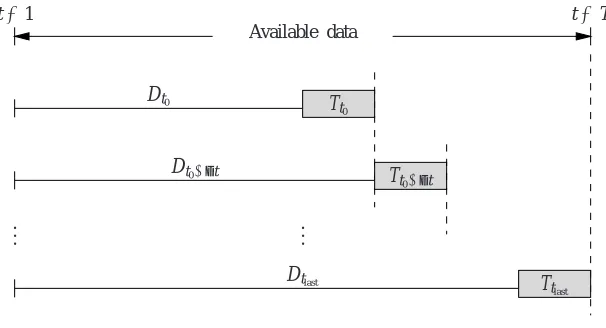
An illustration of the sliding training and test sets is shown in Figure 1.

The most important result of the sequential validation algorithm is the average loss, which can be compared across several algorithms. The individual losses are useful to estimate confidence intervals around the average loss or around differences in average loss (see Section 3.3.2).

In the sequential validation algorithm we would in general prefer to choose∆t=1 but larger

values allow to save computations (in proportion to the value of ∆t). The choice of the training

window size wtdepends on the degree of non-stationarity expected (or estimated) from the particular data sequences. The most common choices are wt=min(w0,t)(a fixed value) and wt=t (use all the available data). Using sequences shorter than t may be justified when the conditional distribution of the data changes so much with t that old training pairs to hurt generalization to new cases. Note that unless wt is constant the amount of training data may change as t increases, thus usually requiring an adaptive model selection algorithm.

3.1 Sequential Validation for Model Selection

.. .

Dt0

Dt0+∆t

t=1 t=T

Dtlast .. . Available data

Tt0

Tt0+∆t

Ttlast

Figure 1: Sliding training and test sets that arise in the sequential validation procedure, where_Dtdenotes a training

set (up to time t),Tt denotes a test set (starting from t), t0is the time of the first test point, and∆tis the

increment between iterations. We assume here a training window size wtof “infinite length”, i.e., which

uses all available past data.

Forecast Horizon

Target to forecast

End of training set Available unlabeled observations

Input value

t

Figure 2: A natural source of unlabeled data for time series forecasting with an horizon arises at the end of the training set.

perform a data-driven model selection. Sequential validation can also be used as a model selec-tion procedure: the funcselec-tion class associated with the lowest validaselec-tion error up to t is chosen for the forecast at t. However, in our experiments we generally found that cross-validation (within the training set) yielded better results for choosing the number of input variables.

3.2 Natural Source of Unlabeled Data

It is also interesting to note that this unlabeled set includes in particular the input for the next test point, xt. This suggests that a method that uses xt for model selection is actually doing a form of transduction. Vapnik introduced in 1982 (see also Vapnik, 1998) the principle of transductive

inference, which differs from the usual inductive inference principle in that the learner chooses a

solution based not only the training set but also on the input values of the test point(s). Here, this is particularly true when the sequential validation step∆t is chosen equal to 1 (which is however more

computationally costly); otherwise, only one out of∆t of the test points would be in U .

Why would it be useful to use the metric model selection methods with the future test points as unlabeled data? The intuition is simply that these are the data points that we care about: this is where we most want to reject functions that “misbehave”.

3.3 Time-Series Transduction Experiments

3.3.1 EXPERIMENTAL SETUP

To verify the potential of metric model selection methods in time-series forecasting applications, we performed feature-selection experiments using artificially-generated data in a controlled setting. Our goal is to compare model selection algorithms (in this case the metric method ADJ against cross-validation) on the set of progressively more complex models that arise in forward (stepwise) feature selection.

Data Generation The artificial data series are generated from the class of linear autoregressive

AR(K) models, where given a fixed coefficients vector α≡(α0,...,αK)0 and initial conditions

y₋1,y−2,...,y−K, we have the process

yt =α0+

K

∑

αkyt−k+εt, t≥0

withεt ∼

N

To simplify matters and ease analysis, we restrict the generating models to the specific form

yt=α+αyt−K+εt, where in our experiments K=1,2,3.

Task Description We seek to forecast the series{yt}at horizon h, given the realizations of the past ˜K series values (we do not impose that ˜K be equal to the order K of the generating process).

One typically considers a point forecast, or in other words, at a given time t and given the values of{yt,yt−1,...,yt−K˜+1}, one seeks an estimator of E[yt+h|

I

yt+1+yt+2+···+yt+h. We shall then seek an estimator of

E[yt+1+yt+2+···+yt+h|

I

In many applications this type of forecast can be interpreted more naturally in terms of the underly-ing problem variables; for instance, given a financial series of (log) returns, the integrated forecast corresponds to the estimated total portfolio (log) return over the horizon. Obviously, at horizon

h=1, the integrated forecast is equivalent to the point forecast.

1. We also performed experiments withεt∼t(5), to evaluate the performance in the presence of an “uglier” fat-tailed

We shall consider the class of AR(K˜) models to make this forecast. This is equivalent to esti-mating the coefficients ˆβ≡(βˆ0,...,βˆK˜)0corresponding to the model

h

∑

yt+j=β0+ ˜

K

∑

βkyt−k+1+εt,

whereεt is i.i.d. Gaussian noise.

The estimation of ˆβ, for a fixed ˜K, is easily performed analytically using the ridge estimator

ˆ

β∗_{= (X}0_X+λI)−1_X0_{Y , where X is the matrix of regressors, Y is the (column-) vector of targets,}

and I is the identity matrix.2 This estimator implicitly uses a squared-error loss function, which is appropriate for our task of estimating a conditional expectation.

Feature Selection The role of feature selection here (see Algorithm 1) is to decide whichαk are significant and should be included in the regression. To this end, we use a standard forward stepwise selection algorithm, in which the individual features are the lagged series values, yt−k,k=0,...,K˜− 1. Forward selection proceeds incrementally, starting from the mean (the lowest-complexity model that we are willing to consider), and at each step adds the feature that minimizes the training error. At a given time step t, we have the following sequence of models produced by the algorithm,

{g(_t0),g_t(1),...,g_t(K˜)},

where g_t(k)is the estimated regression model containing the k “best” features according to forward selection (which are not necessarily the first k lagged series values). The model g(t0)is simply the mean on the current training set (obtained from

I

We observe that this sequence of models forms a total order with respect to complexity, and is thence amenable to selection by metric methods. We exploit this crucial property, which arises naturally from the nature of the forward selection algorithm, in the experiments.

Experimental Plan The experiments measure the relative ability of 10-fold cross-validation ver-sus metric model selection (in this case, ADJ) to select among the sequence of models produced by stepwise selection. We compare the methods across a whole spectrum of parameters, i.e., all permutations of:

• Forecasting horizon h={1,2,5,10,15} • Generating model AR order K={1,2,3}

• Generating model coefficient magnitudeα={0.1,0.3,0.5,0.7,0.9}. This coefficient controls the series signal-to-noise ratio;α=0.1 yields series very close to white noise, whereas series withα=0.9 exhibit much more structure.

Each triplethhorizon,AR order,magnitudeiis henceforth called an experiment.

We fix the maximum model order ˜K=10, and a constant training window size wt =75=t0,

making this a challenging task. The sequential validation increment is∆t =10, and the total length of each generated series is 1000 observations. In addition, each “basis” model g(_tk)is estimated with a small ridge penalty λ=10−14. (This hyperparameter was not tuned extensively, but empirically

produced quite reasonable results.)

3.3.2 STATISTICAL METHODOLOGY

We compare the performance of two models on a given experiment by a usual paired t-test on their mean-squared error difference. However, the results of individual experiments (e.g. across different horizons) cannot be pooled arbitrarily, since the expected error distribution is quite different across experiments. For instance, we expect a priori the MSE to be higher when forecasting across a longer horizon, given a stationary underlying generating process.

To perform a valid statistical test of the performance difference between methods across

exper-iments, it is necessary to normalize the distribution of paired differences within each experiment to

have unit standard deviation, before pooling the observations across experiments, and then perform-ing the statistical test.

More specifically, suppose we perform M experiments, each one with Njtest points. Let eij,j= 1,...,M,i=1,...,Nj be the squared error differences between two methods we wish to compare (e.g. cross-validation against ADJ in our case). The first step is to normalize the distribution of error differences to unit standard deviation,

˜

e_ij= e

j i

p

ˆ σ2(_ej),

where the variance estimator ˆσ2(ej)is described below. Then we compute the overall mean differ-ence ¯e and standard error ˆσe¯as

¯

e= ∑

M j=1∑

Nj

i=1e˜

j i ∑M

j=1Nj

, σˆe¯=

1

q

∑M j=1Nj

.

Throughout this section, the so-obtained mean difference ¯e is termed normalized MSE difference.

Estimation ofσ(ej) The question left open is the estimation of the standard deviation of the error-difference distribution within a single experiment. The usual estimator cannot be used here for it rests upon an i.i.d. assumption, whereas the series we consider exhibit mild to strong autocorrelation patterns. This autocorrelation is induced, on the one hand, by the problem structure, and on the other hand by the sequential validation testing procedure.3

To properly estimate the variance, we use the Newey–West estimator well-known to econo-metricians (Newey and West, 1987, Diebold and Mariano, 1995, Campbell et al., 1997), which in addition to being consistent, has the desirable property of being robust at small sample sizes,4

ˆ

σ2_(ej_{) =ˆγ}j

0+2

q

∑

q−k q ˆγ

j k,

where q is the maximum lag length to be considered,5and ˆγ_kj is the empirical lag-k autocovariance, ˆ

γj k=

1

Nj−k Nj−k

∑

(e_ij−e¯j)(e_ij_+k−e¯j),

with ¯ej the sample mean.

3. Since successive training sets in sequential validation tend to highly overlap, the trained models are generally very correlated—especially at small step sizes∆t—thence inducing correlation in the error structure.

3.3.3 EXPERIMENTAL RESULTS

0.3 0.5 0.7 0.9

AR Coeff. Magnitude

-0.06 -0.04 -0.02 0.02 0.04 0.06 Normalized MSEXV-MSEADJ

2 5 10 15

Forecast Horizon

-0.06 -0.04 -0.02 0.02 Normalized MSEXV-MSEADJ

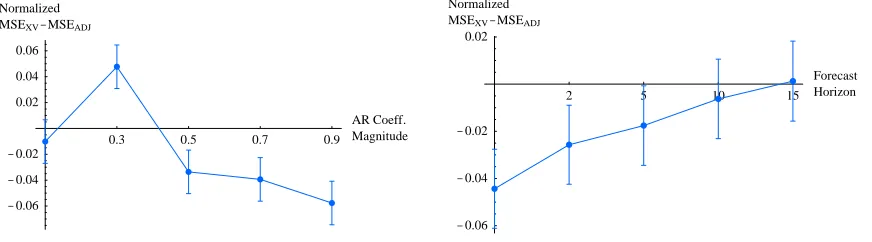
Figure 3: Left: Normalized MSE difference between the models chosen by cross-validation and ADJ, as a func-tion of the magnitude of the AR coefficients (across all forecast horizons and generating model order). The error bars represent 95% confidence intervals on the mean difference (normalized as explained in the

text). Right: Same measure, as a function of the forecast horizon; we note that even with extremely few

unlabeled observations (one or two), ADJ does not lose catastrophically against cross-validation, which is very surprising; the two methods become essentially equivalent for longer horizons.

Figure 3 presents a summary of the experiments described above, comparing cross-validation against ADJ. The left plot outlines the effect of the series signal-to-noise (SNR) ratio (for which the generating model AR coefficient magnitude are a proxy) on performance. At very low SNR, the series being essentially white noise, both methods perform about equally poorly—worse, in fact, than a naive constant model (not shown on the figure). At the other end of the spectrum, at high coefficient values, cross-validation performs, overall, significantly better than ADJ. However, the opposite picture emerges at small but significant coefficient values, where ADJ significantly beats cross-validation. We conjecture that at these moderate SNR levels, the intrinsic variance of the choice made by cross-validation causes costly mistakes, whereas a less-variable (albeit biased) method such as ADJ can pick out important structures without being swamped by the noise level.

The right plot in Figure 3 is, in some ways, more surprising: first, there is a steady improvement in the average performance of ADJ with respect to cross-validation as the forecast horizon increases, because of the increase in the number of unlabeled observations that ADJ can use to make its choice. But the unexpected outcome is, relatively speaking, how well ADJ performs given extremely few

unlabeled observations (one or two); recall that these observations are used to form a Monte Carlo

approximator of an expectation (c.f. Equation 1), and that so few observations are sufficient to make a reasonable model selection choice in this context strikes us as a surprise.

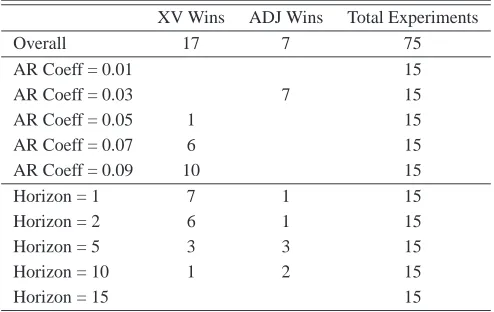
XV Wins ADJ Wins Total Experiments

Overall 17 7 75

AR Coeff = 0.01 15

AR Coeff = 0.03 7 15

AR Coeff = 0.05 1 15

AR Coeff = 0.07 6 15

AR Coeff = 0.09 10 15

Horizon = 1 7 1 15

Horizon = 2 6 1 15

Horizon = 5 3 3 15

Horizon = 10 1 2 15

Horizon = 15 15

Table 1: “Tournament” results comparing cross-validation against ADJ for individual experiments. A “win” indicates that the corresponding method beats the other at a statistical significance level of at least 95% (p≤0.05) on the MSE criterion. A blank stands for zero. The results corroborate those of Figure 3.

4. “Meta” Model Selection

The motivation for this other extension to the metric model selection methods follows from several years of working with various model selection methods and frustratingly comparing them against cross-validation. Cross-validation does not always work but it almost always performs quite well. However, it tends to have higher variance (in the sense of larger variations in error) than complexity penalization methods. We also know that it is almost unbiased (it is unbiased for training with a bit less examples than what is actually available).6 Since it is usually almost as good (and often better) than these complexity penalization methods (including the metric methods), it must mean that these other methods must have smaller variance (and none of them is guaranteed to be unbiased, so they are likely to be biased). Can we take advantage of this situation, whereby one method is more biased but has less variance than the other?

In this paper we have just begun to explore this opportunity. Let us call gxvthe solution obtained

by cross-validation and gp the solution obtained by some form of complexity penalization, for a

particular training set. A simple-minded combination algorithm is the following: if, for a given test point x, the absolute difference|gxv(x)−gp(x)|is “large”, then trust gp, else trust gxv. The intuition for this heuristic rule is that a large difference in function value more likely indicates that the cross-validatory choice is wrong, owing to its large variance. This leaves open the question of choosing the proper threshold. A more sophisticated (and better grounded) algorithm for the squared loss, which we have tested in the experiments is shown in Algorithm 3. We also test a trivial combination algorithm, which takes the simple average of the prediction gxv(x)and the prediction gp(x).

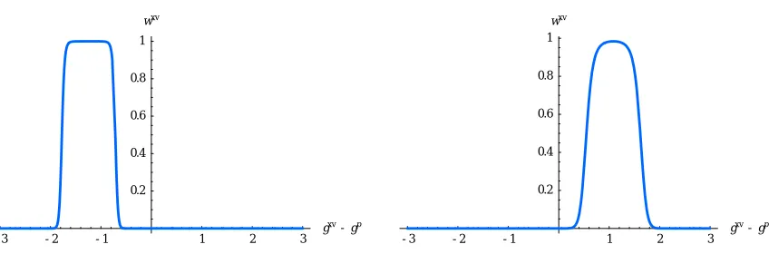
Algorithm 3 is based on the idea of the logistic regression: it assigns a weight ws(β) to the

cross-validation model (and 1−ws(β) to the ADJ model) based on a quadratic function of the

difference gxv(x)−gp(x);7the use of the sigmoid ensures that the weights are always between 0 and 6. We are talking about the bias of an estimator of generalization error. However, for most model selection methods, the

Algorithm 3 Logistic Meta Model Selection

Input at t: the sequence of solutions gxv_s and gsp, respectively for the cross-validation and complexity penalization selected models, and the data sequence{(xs,ys)}for s≤t.

1. Letds:=gxvs (xs)−gps(xs)

2. Letws(β):=1/(1+exp(−(β0+β1ds+β2ds2))) 3. LetC(β):=∑s≤t−h(ws(β)gxvs + (1−ws(β))gsp−ys+h)2 4. Letβ∗:=argmin_βC(β)

Output at t: the solution gt :=wt(β)gxvt + (1−wt(β))gtp.

1. Contrarily to traditional logistic regression, the coefficient vector βfor the weights is obtained by directly optimizing a squared-loss criterion, estimated from the past test observations (i.e., those for s≤t, available without cheating from the sequential validation procedure).

Like Boosting (Freund and Schapire, 1996) and other model combination algorithms, the lo-gistic combination algorithm combines multiple predictors, and it does so in a way that gives more weight to the best predictor. However, the weight changes from example to example, as a learned function of the difference between the two predictors.

4.1 Meta Model Selection Experiments

The same experimental setup as described in Section 3.3.1 was used to compare the logistic com-bination rule against cross-validation alone and ADJ alone. “Tournament” results are shown in Table 2. The most significant observation is that the logistic combination almost always performs

better than either method taken alone. As the table shows, across all experiments, the logistic

combination loses only once to cross-validation and ADJ, whereas it wins more frequently against them.

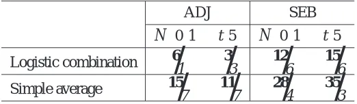
Table 3 shows “tournament” results against cross-validation in the same experimental setting as described above (each tournament made up of the 75 experiments), in various conditions, with

m=75 being the size of the training set and N is the number of features:

• Varying the combination algorithm. We tried both the logistic combination (Algorithm 3)

and an equal-weight combination (simple average) between the two model choices; i.e., in the notation of Algorithm 3, the simple average combination is gt :=1₂gxvt +12g

p t.

• Varying the metric model selection method. We tried both ADJ and the Smallest Eigenvalue Bound (SEB) criterion (Chapelle et al., 2002):

dT(g,PY|X) 1−Nm

₋1

1+_{m k}N with k= (1−

q

N(ln2m N+1)+4

m )+.

• Process innovationsεt either following a normal

N

t(5)distribution.

Logis Wins XV Wins Logis Wins ADJ Wins Total Exp.

Overall 6 1 15 1 75

AR Coeff = 0.01 1 15

AR Coeff = 0.03 6 15

AR Coeff = 0.05 1 3 1 15

AR Coeff = 0.07 3 15

AR Coeff = 0.09 8 15

Horizon = 1 1 7 15

Horizon = 2 1 6 15

Horizon = 5 3 1 2 15

Horizon = 10 1 15

Horizon = 15 1 15

Table 2: “Tournament” results comparing the logistic combination against, respectively cross-validation alone and ADJ alone, for individual experiments. A “win” indicates that the corresponding method beats the other at a statistical significance level of at least 95% (p≤0.05) on the MSE criterion. A blank stands for zero.

ADJ SEB

N

N

Logistic combination 6

/

/

/

/

Simple average 15

/

/

/

/

Table 3: Number of times that each algorithm beats/is beaten by cross-validation, under both a normal and a t distribution, in a total of 75 experiments (described in the text). “Beating”, as in the previous tournament results, is to exhibit a statistically significantly better performance (p<0.05level).

to implement. 2) With ADJ, the logistic combination appears more robust (loses less often to cross-validation alone). 3) The combination of SEB and cross-cross-validation performs very well, better than the combination of ADJ and cross-validation; we conjecture that SEB has an even smaller variance than ADJ (albeit with a possibly worse bias), and this should be the basis of future investigations.

-3 -2 -1 1 2 3 gxv

-gp 0.2

0.4 0.6 0.8 1 wxv

-3 -2 -1 1 2 3

gxv -gp 0.2

0.4 0.6 0.8 1 wxv

Figure 4: Examples of the weight ws(β) given to the cross-validation model ( c.f. Algorithm 3), obtained by the

logistic regression, as a function of the difference gxv−gpevaluated at the test point.

5. Proposed Extension when No Unlabeled Data is Available

The final extension to TRI, ADJ and ADA applies to the case where no unlabeled data is available, which occurs in many applications. The basic idea is to approximate the expected value of d(f,g)

using a model of the input density rather than with an average over unlabeled data,

˜

d(f,g)def=ψ

Z ˆ

PX(x)L(f(x),g(x))dx

,

where ˆPX(x) is the model of the input density. In practice this integral may be difficult to compute analytically so we used a simple Monte-Carlo procedure based on sampling from the density model

ˆ

PX. This model may be derived from the training set input points(x1,...,xm)and/or prior knowledge about the input density. In our experiments we have used a Parzen windows density estimator (that only relies on the data),

ˆ

PX(x)

def

= 1

m

∑

e−0.5||xi−x||2/σ2 (2π)n/2σn ,

where x∈

R

been proposed for setting the smoothing parameter of such non-parametric density estimators. In our

experiments we have experimented with the effect of varyingσand we have used an asymptotically

motivated estimator (Scott, 1992):

σ=1.144

q c

Var[X]

m1/5 , (2)

whereVarc[X]denotes sample variance of the inputs on the training set.

5.1 Extension of Theoretical Results

those results characterize the generalization error measured with respect to the estimated input den-sity ˆPX(x). The main theoretical results are briefly recalled here. Let us call xTRI, xADJ, and xADA the extended methods using ˆPX(x).

Proposition 1 Let gm=argmingid˜(gi,PY|X), and let gl be the hypothesis selected by xTRI. If m≤l and dT(gm,PY|X)≤d˜(gm,PY|X)then ˜d(gl,PY|X)≤3 ˜d(gm,PY|X).

The above tells us when xTRI cannot overfit too much.

Proposition 2 Let gm=argmingid˜(gi,PY|X), and let gl be the hypothesis selected by xADJ. If m≤l and ˆd(gm,PY|X)≤d˜(gm,PY|X))then ˜d(gl,PY|X)≤(2+

dT(gm,PY|X)

dT(gl,PY|X))

˜

d(gm,PY|X). The above tells us when xADJ cannot overfit too much.

Proposition 3 Consider a hypothesis gm, and assume that dT(gl,PY|X)≤d˜(gl,PY|X) for l≤

m, and dT(gl,PY|X) ≤dˆ(gl,PY|X) for l ≤m. Then if ˜d(gm,PY|X)≤ 13

dT(gl,PY|X)2 ˜

d(gl,PY|X) for l <m (i.e.,

˜

d(gm,PY|X) is sufficiently small) it follows that ˆd(gm,PY|X)<dˆ(gl,PY|X) for l<m and therefore xADJ will not choose any predecessor in lieu of gm.

The above tells us when xADJ cannot underfit too much. See Schuurmans and Southey (2002) for proofs of equivalent results for the original methods, and detailed discussions. The same au-thors observe that the conditions required for these propositions to hold are not always satisfied in practice.

5.2 Experimental Results

5.2.1 ARTIFICIALDATARESULTS

To ascertain the validity of the proposed extensions, we first performed experiments on artificial data, keeping the same overall framework as Schuurmans and Southey (2002). We tested the meth-ods on data generated from the four following functions:

f1(x) =1x≥0.5 f3(x) =sin2(2πx)

f2(x) =sin(1/x) f4(x) =32x−275x2+777x3−892x4+358x5 Our class of nested models is the set of polynomials of fixed order,

g(x;β) =

m

∑

βjxj,

where the order m depends on the size of the training set (described below). The models are trained to minimize a squared error criterion with weight decay; the members of the class vary according to the value of the weight-decay coefficientλ(a higherλimplies a reduced capacity). We restrictedλ to the set{10i_{: i=−5,−4.5,−4,... ,2}, which was found to be adequate. The optimal parameter} vector ˆβ∗is given by the well-known ridge estimator, ˆβ∗= (X0X+λI)−1X0Y , where X is the matrix

of regressors, Y is the (column-) vector of targets, and I is the identity matrix.

The artificial data sets are generated from the functions f1,...,f4. The input density PX(x) is chosen as either uniform on the [0,1] interval (U(0,1)), or normal with mean 1₂ and variance ₁₂1 (

N

2, 1

12), chosen to have the same mean and variance as the U(0,1)distribution). Additive noise

with a distribution

N

Like Schuurmans and Southey (2002), we consider training sets of sizes{10,20,30}. The size

15 20 25 30 Train size

-3

-2

-1

MSE Log-Ratio _{Target function: f3}

15 20 25 30 Train size

-1.25

-1

-0.75

-0.5

-0.25 0.25

MSE Log-Ratio _{Target function: f4}

15 20 25 30 Train size

-3

-2

-1 1 2

MSE Log-Ratio _{Target function: f1}

15 20 25 30 Train size

-3

-2

-1

MSE Log-Ratio Target function: f2

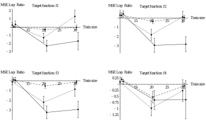
Figure 5: Comparison between Parzen-generated unlabeled data and “true” unlabeled data, for xTRI/TRI (dotted line), xADJ/ADJ (dashed line), and xADA/ADA (solid line). Each point is the median test MSE log-ratio of 50 repetitions, with random training, unlabeled and test sets; the error bars represent 1 standard error on the median, computed by bootstrap resampling. The input distribution is_N(1₂,₁₂1). Surprisingly, the Parzen-generated data sometimes performs significantly better (negative log-ratio) than unlabeled data from “true”

PX(x), and never significantly worse.

number of unlabeled examples are sampled from the Parzen estimator for xTRI, xADJ, and xADA. Finally, a single test set of size 5000 is generated to evaluate performance.

Figure 5 compares each method against 10-fold cross-validation. We observe that the proposed methods compare favorably to the originals, sometimes beating them at a statistical significance level above 95%.

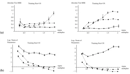
Figure 6 shows the effect of the Parzen estimator bandwidthσ. Panel (a) shows the sensitivity

of the median MSE of the three algorithms toσ; xADA is the least sensitive to the choice of σ.

Panel (b) shows the sensitivity of the log-norm of the parameters (i.e., reflecting the complexity of the solution) with respect toσ. In most cases, as we expected, a higherσyields simpler solutions.

However, unexpectedly, we find in one case that largerσyields larger parameters (for xADA).

5.2.2 RESULTS ON THEBOSTON HOUSING DATASET

(a) 0.5 1 1.5 2 sigma multiplier 0.2 0.4 0.6 0.8 1 1.2 1.4

Absolute Test MSE _{Training Size=10}

0.5 1 1.5 2

sigma multiplier 0.2 0.4 0.6 0.8 1 1.2 1.4

Absolute Test MSE _{Training Size=30}

(b) 0.5 1 1.5 2

sigma multiplier -1 1 2 3 4 Log-Norm of

Parameters _{Training Size=10}

0.5 1 1.5 2

sigma multiplier -1 1 2 3 4 5 Log-Norm of

Parameters _{Training Size}=30

Figure 6: Effect of Parzen estimator window width for xTRI (dotted line), xADJ (dashed line), and xADA (solid line). Panel (a) shows the median MSE performance; we observe that xTRI is very sensitive to the window

width, xADJ less to, and that xADA is nearly insensitive to it. Panel (b) shows the log-norm of the

parameters of the trained models; we note that the window width has a clear regularization effect for xTRI

and xADJ. In both cases, the window width is given as a multiplicative factor applied to Equation (2).

All results are computed for function f1 under a U(0,1)input distribution, 50 repetitions. The error bars represent 1 standard error on the median and the mean respectively.

RBF per training example:

g(z;σ) =

m

∑

wiexp

−kz−xik2 2σ2

,

where {xi}mi=1 are the training set inputs, and σ is the RBF window width.8 For a given weight

decayλ, an analytical solution for the withat minimizes the squared error criterion is easily obtained (similar to the ridge estimator presented in Section 5.2.1).

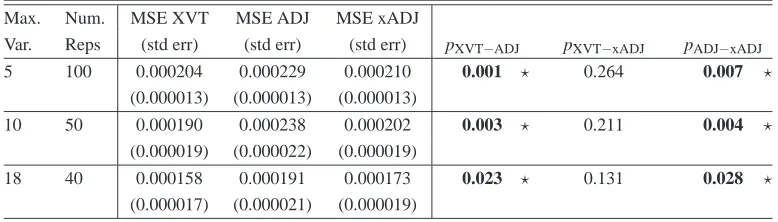
We used a standard forward stepwise feature selection procedure (as described in algorithm 1 and Section 3.3.1) to obtain a nested family of models of increasing complexity. We then use a model selection algorithm to select the best-performing model among this family. Table 4 compares the performance of cross-validation (XVT), ADJ, and xADJ on the Boston dataset (506 observations with no missing values, 18 features, 1 continuous target). The difficulty of the model selection problem is controlled by the maximum allowed number of features; we compared the performance allowing a maximum of 5, 10, and 18 features.

The results indicate that both cross-validation and xADJ perform, on average, significantly bet-ter than plain ADJ. This is surprising, since the latbet-ter has access to more information (303 unlabeled

Max. Num. MSE XVT MSE ADJ MSE xADJ

Var. Reps (std err) (std err) (std err) pXVT−ADJ pXVT−xADJ pADJ−xADJ

5 100 0.000204 0.000229 0.000210 0.001 ? 0.264 0.007 ?

(0.000013) (0.000013) (0.000013)

10 50 0.000190 0.000238 0.000202 0.003 ? 0.211 0.004 ?

(0.000019) (0.000022) (0.000019)

18 40 0.000158 0.000191 0.000173 0.023 ? 0.131 0.028 ?

(0.000017) (0.000021) (0.000019)

Table 4: Comparing cross-validation (XVT), ADJ, and xADJ on the UCI Boston Housing dataset. The table reports the average Test MSE and standard errors, within the Forward Feature Selection setting described in the text. Max. Var. is the maximum number of features allowed in the forward selection procedure. To obtain standard errors, random (nonoverlapping) training (size=101), unlabeled (size=303), and test (size=102) sets are drawn, Num. Rep. times (which differs depending on Max. Var. for computation time reasons). The three rightmost columns give the p-values that the paired MSE difference between the indicated algorithms is zero, under the appropriate t-distribution. We note that plain ADJ is always significantly worse than either XVT and xADJ, and no significant difference is found between the latter two. The underlying Boston dataset contains 506 observations with no missing values. The learning algorithm is an RBF network with constant

weight decay=10−2, gaussian window width=1, and one RBF per training point.

observations from the “true” distribution). Furthermore, xADJ never performs significantly worse than cross-validation. In all cases, 300 unlabeled observations were generated from the Parzen distribution for xADJ. The differences between ADJ and xADJ could just be due a statistical fluc-tuation occuring with the particular data used in the experiments. However, since we do not fully understand the nature of the generalization improvement brought by ADJ and xADJ there could also be another explanation, which future work should investigate.

6. Conclusions

We have presented three new model and feature selection methods, with the goals of improving and extending the applicability of metric-based methods.

A first surprising result is that ADJ can work with time-series data (and not be beaten by cross-validation in the majority of cases) in a transductive fashion while using only as few as 1 to 10 unlabeled examples (whereas one would have expected that with so few examples the complexity correction computed by ADJ would be very unreliable).

A second surprising result is that using non-parametric density estimators, ADJ can be succes-fully applied even when an independent source of unlabeled data is not available.

References

Y. Bengio and D. Schuurmans. Special issue on new methods for model selection and model com-bination, 2002. Machine Learning, 48(1).

J. Y. Campbell, A. W. Lo, and A. C. MacKinlay. The Econometrics of Financial Markets. Princeton University Press, Princeton, 1997.

O. Chapelle, V. N. Vapnik, and Y. Bengio. Model selection for small-sample regression. Machine

Learning Journal, 48(1):9–23, 2002.

O. Chapelle, J. Weston, L. Bottou, and V. N. Vapnik. Vicinal risk minimization. In T.K. Leen, T.G. Dietterich, and V. Tresp, editors, Advances in Neural Information Processing Systems, volume 13, pages 416–422, 2001.

F. X. Diebold and R. S. Mariano. Comparing predictive accuracy. Journal of Business and Economic

Statistics, 13(3):253–263, 1995.

D. Foster and E. George. The risk inflation criterion for multiple regression. Annals of Statistics, 22:1947–1975, 1994.

Y. Freund and R. E. Schapire. Experiments with a new boosting algorithm. In Machine Learning:

Proceedings of Thirteenth International Conference, pages 148–156, 1996.

W. Newey and K. West. A simple, positive semi-definite, heteroscedasticity and autocorrelation consistent covariance matrix. Econometrica, 55:703–708, 1987.

T. Poggio and F. Girosi. Regularization algorithms for learning that are equivalent to multilayer networks. Science, 247:978–982, 1990.

J. Rissanen. Stochastic complexity and modeling. Annals of Statistics, 14:1080–1100, 1986.

D. Schuurmans. A new metric-based approach to model selection. In Proceedings of the National

Conference on Artificial Intelligence (AAAI-97), pages 552–558, 1997.

D. Schuurmans and F. Southey. Metric-based methods for adaptive model selection and regulariza-tion. Machine Learning, 48(1):51–84, 2002.

D. W. Scott. Multivariate Density Estimation: Theory, Practice, and Visualization. Wiley, New York, 1992.

V. N. Vapnik. Statistical Learning Theory. Wiley, Lecture Notes in Economics and Mathematical Systems, volume 454, 1998.