Variational Inference for Latent Variables and Uncertain
Inputs in Gaussian Processes
Andreas C. Damianou∗ [email protected]
Dept. of Computer Science and Sheffield Institute for Translational Neuroscience University of Sheffield
UK
Michalis K. Titsias∗ [email protected]
Department of Informatics
Athens University of Economics and Business Greece
Neil D. Lawrence [email protected]
Dept. of Computer Science and Sheffield Institute for Translational Neuroscience University of Sheffield
UK
Editor:Amos Storkey
Abstract
The Gaussian process latent variable model (GP-LVM) provides a flexible approach for non-linear dimensionality reduction that has been widely applied. However, the current approach for training GP-LVMs is based on maximum likelihood, where the latent projec-tion variables are maximised over rather than integrated out. In this paper we present a Bayesian method for training GP-LVMs by introducing a non-standard variational inference framework that allows to approximately integrate out the latent variables and subsequently train a GP-LVM by maximising an analytic lower bound on the exact marginal likelihood. We apply this method for learning a GP-LVM from i.i.d. observations and for learning non-linear dynamical systems where the observations are temporally correlated. We show that a benefit of the variational Bayesian procedure is its robustness to overfitting and its ability to automatically select the dimensionality of the non-linear latent space. The result-ing framework is generic, flexible and easy to extend for other purposes, such as Gaussian process regression with uncertain or partially missing inputs. We demonstrate our method on synthetic data and standard machine learning benchmarks, as well as challenging real world datasets, including high resolution video data.
Keywords: Gaussian processes, variational inference, latent variable models, dynamical systems, uncertain inputs
1. Introduction
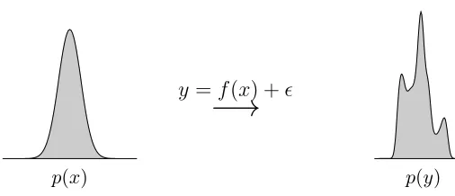
Consider a non linear function, f(x). A very general class of probability densities can be recovered by mapping a simpler density through the non linear function. For example, we
p(y)
p(x)
y=f(x) +
−→
Figure 1: A Gaussian distribution propagated through a non-linear mapping. yi =f(xi) +
i. ∼ N 0,0.22
andf(·) uses RBF basis, 100 centres between -4 and 4 and`= 0.1. The new distribution overy (right) is multimodal and difficult to normalize.
might decide thatx should be drawn from a Gaussian density
x∼ N(0,1)
and we observey, which is given by passing samples fromxthrough a non linear function, perhaps with some corrupting noise
y=f(x) +, (1)
wherecould also be drawn from a Gaussian density
∼ N 0, σ2,
this time with variance σ2. Whilst the resulting density for y, denoted by p(y), can now have a very general form, these models present particular problems in terms of tractability.
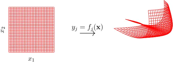
Models of this form appear in several domains. They can be used for nonlinear di-mensionality reduction (MacKay, 1995; Bishop et al., 1998) where several latent variables,
x={xj}qj=1 are used to represent a high dimensional vector y={yj}pj=1 and we normally have p > q,
y=f(x) +.
They can also be used for prediction of a regression model output when the input is uncertain (see e.g. Oakley and O’Hagan, 2002) or for autoregressive prediction in time series (see e.g. Girard et al., 2003). Further, by adding a dynamical autoregressive component to the non-linear dimensionality reduction approaches leads to non-linear state space models (S¨arkk¨a, 2013), where the states often have a physical interpretation and are propagated through time in an autoregressive manner:
xt=g(xt−1),
where g(·) is a vector valued function. The observations are then observed through a separate nonlinear vector valued function,
x2
x1
yj =fj(x)
−→
Figure 2: A three dimensional manifold formed by mapping from a two dimensional space to a three dimensional space.
The intractabilities of mapping a distribution through a non-linear function have re-sulted in a range of different approaches. In density networks sampling was proposed; in particular, in (MacKay, 1995)importance sampling was used. When extending importance samplers dynamically, the degeneracy in the weights needs to be avoided, thus leading to the resampling approach suggested for the bootstrap particle filter of Gordon et al. (1993). Other approaches in non-linear state space models include the Laplace approximation as used in extended Kalman filters and unscented and ensemble transforms (see S¨arkk¨a, 2013). In dimensionality reduction the generative topographic mapping (GTM Bishop et al., 1998) reinterpreted the importance sampling approach of MacKay (1995) as a mixture model, using a discrete representation of the latent space.
In this paper we suggest a variational approach to dealing with latent variables and input uncertainty that can be applied to Gaussian process models. Gaussian processes provide a probabilistic framework for performing inference over functions. A Gaussian process prior can be combined with a data set (through an appropriate likelihood) to obtain a posterior process that represents all functions that are consistent with the data and our prior.
Our initial focus will be application of Gaussian process models in the context of di-mensionality reduction. In didi-mensionality reduction we assume that our high dimensional data set is really the result of some low dimensional control signals which are, perhaps, non-linearly related to our observed functions. In other words we assume that our data,
Y ∈ <n×p, can be generated by a lower dimensional matrix, X ∈ <n×q through a vector
valued function where each row,yi,:ofYrepresents an observed data point and is generated through
yi,:=f(xi,:) +i,:,
so that the data is a lower dimensional subspace immersed in the original, high dimensional space. If the mapping is linear, e.g. f(xi,:) =Wxi,: withW∈ <q×p, methods like principal
In the context of dimensionality reduction a range of approaches have been suggested that consider neighbourhood structures or the preservation of local distances to find a low dimensional representation. In the machine learning community, spectral methods such as isomap (Tenenbaum et al., 2000), locally linear embeddings (LLE, Roweis and Saul, 2000) and Laplacian eigenmaps (Belkin and Niyogi, 2003) have attracted a lot of attention. These spectral approaches are all closely related to kernel PCA (Sch¨olkopf et al., 1998) and classical multi-dimensional scaling (MDS) (see e.g. Mardia et al., 1979). These methods do have a probabilistic interpretation as described by Lawrence (2012) which, however, does not explicitly include an assumption of underlying reduced data dimensionality. Other iterative methods such as metric and non-metric approaches to MDS (Mardia et al., 1979), Sammon mappings (Sammon, 1969) and t-SNE (van der Maaten and Hinton, 2008) also lack an underlying generative model.
Probabilistic approaches, such as the generative topographic mapping (GTM, Bishop et al., 1998) and density networks (MacKay, 1995), view the dimensionality reduction prob-lem from a different perspective, since they seek a mapping from a low-dimensional latent space to the observed data space (as illustrated in Figure 2), and come with certain advan-tages. More precisely, their generative nature and the forward mapping that they define, allows them to be extended more easily in various ways (e.g. with additional dynamics modelling), to be incorporated into a Bayesian framework for parameter learning and to handle missing data. This approach to dimensionality reduction provides a useful archetype for the algorithmic solutions we are providing in this paper, as they require approximations that allow latent variables to be propagated through a non-linear function.
Our framework takes the generative approach prescribed by density networks and the non-linear variants of Kalman filters one step further. Because, rather than considering a specific function, f(·), to map from the latent variables to the data space, we will consider an entire family of functions. One that subsumes the more restricted class of either Gauss Markov processes (such as thelinear Kalman filter/smoother) and Bayesian basis function models (such as the RBF network used in the GTM, with a Gaussian prior over the basis function weightings). These models can all be cast within the framework of Gaussian processes (Rasmussen and Williams, 2006). Gaussian processes are probabilistic kernel methods, where the kernel has an interpretation of a covariance associated with a prior density. This covariance specifies a distribution over functions that subsumes the special cases mentioned above.
In this paper we formulate a variational inference framework which allows us to prop-agate uncertainty through a Gaussian process and obtain a rigorous lower bound on the marginal likelihood of the resulting model. The procedure followed here is non-standard, as computation of a closed-form Jensen’s lower bound on the true log marginal likelihood of the data is infeasible with classical approaches to variational inference. Instead, we build on, and significantly extend, the variational GP method of Titsias (2009), where the GP prior is augmented to include auxiliary inducing variables so that the approximation is ap-plied on an expanded probability model. The resulting framework defines a bound on the evidence of the GP-LVM which, when optimised, gives as a by-product an approximation to the true posterior distribution of the latent variables given the data.
Considering a posterior distribution rather than point estimates for the latent points means that our framework is generic and can be easily extended for multiple practical scenarios. For example, if we treat the latent points as noisy measurements of given inputs we obtain a method for Gaussian process regression with uncertain inputs (Girard et al., 2003) or, in the limit, with partially observed inputs. On the other hand, considering a latent space prior that depends on a time vector, allows us to obtain a Bayesian model for dynamical systems (Damianou et al., 2011) that significantly extends classical Kalman filter models with a non-linear relationship between the state space, X, and the observed data Y, along with non-Markov assumptions in the latent space which can be based on continuous time observations. This is achieved by placing a Gaussian process prior on the latent space, X which is itself a function of time, t. This approach can itself be trivially further extended by replacing the time dependency of the prior for the latent space with a spatial dependency, or a dependency over an arbitrary number of high dimensional inputs. As long as a valid covariance function1 can be derived (this is also possible for strings and graphs). This leads to a Bayesian approach for warped Gaussian process regression (Snelson et al., 2004; L´azaro-Gredilla, 2012).
In the next subsection we summarise the notation and conventions used in this paper. In Section 2 we review the main prior work on dealing with latent variables in the context of Gaussian processes and describe how the model was extended with a dynamical component. We then introduce the variational framework and Bayesian training procedure in Section 3. In Section 4 we describe how the variational approach is applied to a range of predictive tasks and this is demonstrated with experiments conducted on simulated and real world datasets in Section 5. In Section 6 we discuss and experimentally demonstrate natural but important extensions of our model, motivated by situations where the inputs to the GP are not fully unobserved. These extensions give rise to an auto-regressive variant for performing iterative future predictions, as well as a GP regression variant which can handle missing inputs. Finally, based on the theoretical and experimental results of our work, we present our final conclusions in Section 7. This article builds on and extends the previously published conference papers in (Titsias and Lawrence, 2010; Damianou et al., 2011).
1.1 Notation
Throughout this paper we use capital boldface letters to denote matrices, lower-case boldface letters to denote vectors and lower-case letters to denote scalar quantities. We denote the
ith row of the matrix Y as yi,: and its jth column as y:,j, whereas yi,j denotes the scalar
element found in theith row andjth column ofY. We assume that data points are stored by rows, so that thep−dimensional vectoryi,:corresponds to theith data point. The collection of test variables (i.e. quantities given at test time for making predictions) is denoted using an asterisk, e.g.Y∗ which has columns {y∗,j}pj=1.
Concerning variables of interest,Y is the collection of observed outputs,Fis the collec-tion of latent GP funccollec-tion instantiacollec-tions andXis the collection of latent inputs. Further on we will introduce auxiliary inputs denoted byXu, auxiliary function instantiations denoted
by U, a time vector denoted by t, and arbitrary (potentially partially) observed inputs denoted by Z.
If a function f follows a Gaussian process, we use kf to denote its covariance function
andKf f to denote the covariance matrix obtained by evaluatingkf on all available training inputs. The notation θf then refers to the hyperparameters of kf.
2. Gaussian Processes with Latent Variables as Inputs
This section provides background material on current approaches for learning using Gaus-sian process latent variable models (GP-LVMs). Specifically, Section 2.1 specifies the general structure of such models, Section 2.2 reviews the standard GP-LVM for i.i.d. data as well as dynamic extensions suitable for sequence data. Finally, Section 2.3 discusses the drawbacks of MAP estimation over the latent variables which is currently the standard way to train GP-LVMs.
2.1 Gaussian Processes for Latent Mappings
The unified characteristic of all GP-LVM algorithms, as they were first introduced by Lawrence (2005, 2004), is the consideration of a Gaussian Process as a prior distribution for the mapping function f(x) = (f1(x), . . . , fp(x)) so that
fj(x)∼ GP(0, kf(x,x0)), j = 1, . . . , p. (2)
Here, the individual components of f(x) are taken to be independent draws from a Gaus-sian process with kernel or covariance functionkf(x,x0), which determines the properties of
the latent mapping. As shown in (Lawrence, 2005) the use of a linear covariance function makes GP-LVM equivalent to traditional PPCA. On the the other hand, when non-linear covariance functions are considered the model is able to perfom non-linear dimensional-ity reduction. The non-linear covariance function considered in (Lawrence, 2005) is the exponentiated quadratic (RBF),
kf(rbf)(xi,:,xk,:) =σ2rbfexp
−
1 2`2
q
X
j=1
(xi,j −xk,j)2
, (3)
mapping from the latent to the data space. Parameters that appear in a covariance function, such as σrbf2 and`2, are often referred to as kernel hyperparameters and will be denoted by θf.
Given the independence assumption across dimensions in equation (2), the latent vari-ables F ∈ <n×p (with columns {f:,j}pj=1), which have one-to-one correspondence with the data points Y, follow the prior distribution p(F|X,θf) = Qpj=1p(f:,j|X,θf), where p(f:,j|X,θf) is given by
p(f:,j|X,θf) =N(f:,j|0,Kf f) =|2πKf f|−
1
2 exp
−1
2f
>
:,jK−1f ff:,j
, (4)
and whereKf f =kf(X,X) is the covariance matrix defined by the kernel functionkf. The
inputs X in this kernel matrix are latent random variables following a prior distribution
p(X|θx) with hyperparametersθx. The structure of this prior can depend on the application
at hand, such as on whether the observed data are i.i.d. or have a sequential dependence. For the remaining of this section we shall leave p(X|θx) unspecified so that to keep our
discussion general while specific forms for it will be given in the next section.
Given the construction outlined above, the joint probability density over the observed data and all latent variables is written as follows:
p(Y,F,X|θf,θx, σ2) =p(Y|F, σ2)p(F|X,θf)p(X|θx)
=
p
Y
j=1
p(y:,j|f:,j, σ2)p(f:,j|X,θf)p(X|θx),
(5)
where the term
p(Y|F, σ2) =
p
Y
j=1
N y:,j|f:,j, σ2In (6)
comes directly from the assumed noise model of equation (1) whilep(F|X,θf) andp(X|θx)
come from the GP and the latent space. As discussed in detail in Section 3.1, the interplay of the latent variables (i.e. the latent matrix Xthat is passed as input in the latent matrix
F) makes inference very challenging. However, when fixing X we can treat Fanalytically and marginalise it out as follows:
p(Y|X)p(X) =
Z
p(Y|F)p(F|X)dF
p(X),
where
p(Y|X) =
p
Y
j=1
N y:,j|0,Kf f+σ2In
.
Here (and for the remaining of the paper), we omit reference to the parameters θ =
{θf,θx, σ2} in order to simplify our notation. The above partial tractability of the model
gives rise to a straightforward MAP training procedure where the latent inputs X are se-lected according to
XMAP= arg max
This is the approach suggested by Lawrence (2005, 2006) and subsequently followed by other authors (Urtasun and Darrell, 2007; Ek et al., 2008; Ferris et al., 2007; Wang et al., 2008; Ko and Fox, 2009c; Fusi et al., 2013; Lu and Tang, 2014). Finally, notice that point estimates over the hyperparametersθ can also be found by maximising the same objective function.
2.2 Different Latent Space Priors and GP-LVM Variants
Different GP-LVM algorithms can result by varying the structure of the prior distribution
p(X) over the latent inputs. The simplest case, which is suitable for i.i.d. observations, is obtained by selecting a fully factorised (across data points and dimensions) latent space prior:
p(X) =
n
Y
i=1
N(xi,:|0,Iq) = n
Y
i=1 q
Y
j=1
N (xi,j|0,1). (7)
More structured latent space priors can also be used that could incorporate available in-formation about the problem at hand. For example, Urtasun and Darrell (2007) add dis-criminative properties to the GP-LVM by considering priors which encapsulate class-label information. Other existing approaches in the literature seek to constrain the latent space via a smooth dynamical prior p(X) so as to obtain a model for dynamical systems. For example, Wang et al. (2006, 2008) extend GP-LVM with a temporal prior which encapsu-lates the Markov property, resulting in an auto-regressive model. Ko and Fox (2009b, 2011) further extend these models for Bayesian filtering in a robotics setting, whereas Urtasun et al. (2006) consider this idea for tracking. In a similar direction, Lawrence and Moore (2007) consider an additional temporal model which employs a GP prior that is able to generate smooth paths in the latent space.
In this paper we shall focus on dynamical variants where the dynamics are regressive, as in (Lawrence and Moore, 2007). In this setting, the data are assumed to be a multivariate timeseries {yi,:, ti}ni=1 where ti ∈ <+ is the time at which the datapoint yi,: is observed.
A GP-LVM dynamical model is obtained by defining a temporal latent function x(t) = (x1(t), . . . , xq(t)) where the individual components are taken to be independent draws from
a Gaussian process,
xj(t)∼ GP(0, kx(t, t0)), j= 1, . . . , q,
wherekx(t, t0) is the covariance function. The datapointyi,:is assumed to be produced via the latent vectorxi,:=x(ti), as shown in Figure 3(c). All these latent vectors can be stored in the matrix X (exactly as in the i.i.d. data case) which now follows the correlated prior distribution,
p(X|t) =
q
Y
j=1
p(x:,j|t) =
q
Y
j=1
N (x:,j|0,Kx),
whereKx=kx(t,t) is the covariance matrix obtained by evaluating the covariance function
kx on the observed timest. In contrast to the fully factorised prior in (7), the above prior
couples all elements in each column of X. The covariance function kx has parameters θx
an Ornstein-Uhlenbeck covariance function (Uhlenbeck and Ornstein, 1930) yields a Gauss-Markov process forxj(t), while the exponentiated quadratic covariance function gives rise to very smooth and non-Markovian process. The specific choices and forms of the covariance functions used in our experiments are discussed in Section 5.1.
2.3 Drawbacks of the MAP Training Procedure
Current GP-LVM based models found in the literature rely on MAP training procedures, discussed in Section 2.1, for optimising the latent inputs and the hyperparameters. However, this approach has several drawbacks. Firstly, the fact that it does not marginalise out the latent inputs implies that it could be sensitive to overfitting. Further, the MAP objective function cannot provide any insight for selecting the optimal number of latent dimensions, since it typically increases when more dimensions are added. This is why most existing GP-LVM algorithms require the latent dimensionality to be either set by hand or selected with cross-validation. The latter case renders the whole training computationally slow and, in practice, only a very limited subset of models can be explored in a reasonable time.
As another consequence of the above, the current GP-LVMs employ simple covariance functions (typically having a common lengthscale over the latent input dimensions as the one in equation (3)) while more complex covariance functions, that could help to automatically select the latent dimensionality, are not popular. Such a latter covariance function can be an exponentiated quadratic, as in (3), but with different lengthscale per input dimension,
kf(ard)(xi,:,xk,:) =σard2 exp
−
1 2
q
X
j=1
(xi,j−xk,j)2 lj2
, (8)
where the squared inverse lengthscale per dimension can be seen as a weight, i.e. l12
j =wj. This covariance function could thus allow an automatic relevance determination (ARD) procedure to take place, during which unnecessary dimensions of the latent space X are assigned a weight wj with value almost zero. However, with the standard MAP training approach the benefits of Bayesian shrinkage using the ARD covariance function cannot be realised, as typically overfitting will occur; this is later demonstrated in Figure 5. This is the reason why standard GP-LVM approaches in the literature avoid the ARD covariance function and are sensitive to the selection ofq.
principle (Mitchell and Beauchamp, 1988), which provides “hard” shrinkage so that unnec-essary dimensions are assigned a weight exactly equal to zero. This alternative constitutes a promising direction for future research in the context of GP-LVMs.
Given the above, it is clear that the development of fully Bayesian approaches for training GP-LVMs could make these models more reliable and provide rigorous solutions to the limitations of MAP training. The variational method presented in the next section is such an approach that, as demonstrated in the experiments, shows great ability in avoiding overfitting and permits automatic soft selection of the latent dimensionality.
3. Variational Gaussian Process Latent Variable Models
In this section we describe in detail our proposed method which is based on a non-standard variational approximation that uses auxiliary variables. The resulting class of algorithms will be referred to asVariational Gaussian Process Latent Variable Models, or simply vari-ational GP-LVMs.
We start with Section 3.1 where we explain the obstacles we need to overcome when applying variational methods to the GP-LVM and specifically why the standard mean field approach is not immediately tractable. In Section 3.2, we show how the use of auxiliary variables together with a certain variational distribution results in a tractable approxima-tion. In Section 3.3 we give specific details about how to apply our framework to the two different GP-LVM variants that this paper is concerned with: the standard GP-LVM and the dynamical/warped one. Finally, we outline two extensions of our variational method that enable its application in more specific modelling scenarios. In the end of Section 3.3.2 we explain how multiple independent time-series can be accommodated within the same dynamical model and in Section 3.4 we describe a simple trick that makes the model (and, in fact, any GP-LVM model) applicable to vast dimensionalities.
3.1 Standard Mean Field is Challenging for GP-LVM
A Bayesian treatment of the GP-LVM requires the computation of the log marginal likeli-hood associated with the joint distribution of equation (5). Both sets of unknown random variables have to be marginalised out: the mapping values F (as in the standard model) and the latent space X. Thus, the required integral is written as
logp(Y) = log
Z
p(Y,F,X)dXdF= log
Z
p(Y|F)p(F|X)p(X)dXdF (9)
= log
Z
p(Y|F)
Z
p(F|X)p(X)dX
dF. (10)
The key difficulty with this Bayesian approach is propagating the prior densityp(X) through the non-linear mapping. Indeed, the nested integral in equation (10) can be written as
Z
p(X)
p
Y
j=1
where each term p(f:,j|X), given by (4), is proportional to |Kf f|−12 exp
−12f:,j>K−1f ff:,j
. Clearly, this term containsX, which are the inputs of the kernel matrixKf f, in a complex,
non-linear manner and therefore analytical integration overX is infeasible.
To make progress we can invoke the standard variational Bayesian methodology (Bishop, 2006) to approximate the marginal likelihood of equation (9) with a variational lower bound. We introduce a factorised variational distribution over the unknown random variables,
q(F,X) =q(F)q(X),
which aims at approximating the true posterior p(F|Y,X)p(X|Y). Based on Jensen’s in-equality, we can obtain the standard variational lower bound on the log marginal likelihood
logp(Y)≥
Z
q(F)q(X) logp(Y|F)p(F|X)p(X)
q(F)q(X) dFdX. (11) Nevertheless, this standard mean fieldapproach remains problematic because the lower bound above is still intractable to compute. To isolate the intractable term, observe that (11) can be written as
logp(Y)≥
Z
q(F)q(X) logp(F|X)dFdX+
Z
q(F)q(X) logp(Y|F)p(X)
q(F)q(X) dFdX, where the first term of the above equation contains the expectation of logp(F|X) under the distributionq(X). This requires an integration overX which appears non-linearly in K−1f f
and log|Kf f|and cannot be done analytically. Therefore, standard mean field variational methodologies do not lead to an analytically tractable variational lower bound.
3.2 Tractable Lower Bound by Introducing Auxiliary Variables
In contrast, our framework allows us to compute a closed-form lower bound on the marginal likelihood by applying variational inference after expanding the GP prior so as to include auxiliary inducing variables. Originally, inducing variables were introduced for computa-tional speed ups in GP regression models (Csat´o and Opper, 2002; Seeger et al., 2003; Csat´o, 2002; Snelson and Ghahramani, 2006; Qui˜nonero Candela and Rasmussen, 2005; Titsias, 2009). In our approach, these extra variables will be used within the variational sparse GP framework of Titsias (2009).
More specifically, we expand the joint probability model in (5) by including m extra samples (inducing points) of the GP latent mapping f(x), so that ui,: ∈ Rp is such a
sample. The inducing points are collected in a matrix U ∈ Rm×p and constitute latent function evaluations at a set of pseudo-inputsXu∈Rm×q. The augmented joint probability
density takes the form
p(Y,F,U,X|Xu) =p(Y|F)p(F|U,X,Xu)p(U|Xu)p(X)
=
p
Y
j=1
p(y:,j|f:,j)p(f:,j|u:,j,X,Xu)p(u:,j|Xu)
where
p(f:,j|u:,j,X,Xu) =N (f:,j|aj,Σf) (13) is the conditional GP prior (see e.g. Rasmussen and Williams (2006)), with
aj =Kf uK−1uuu:,j(with ai,j =kf(xi,:,Xu)K−1uuu:,j) and Σf =Kf f−Kf uK−1uuKuf. (14)
Further,
p(u:,j|Xu) =N(u:,j|0,Kuu) (15) is the marginal GP prior over the inducing variables. In the above expressions,Kuudenotes
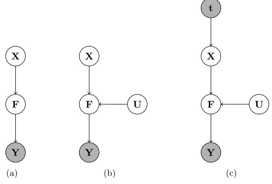
the covariance matrix constructed by evaluating the covariance function on the inducing points, Kuf is the cross-covariance between the inducing and the latent points andKf u= K>uf. Figure 3(b) graphically illustrates the augmented probability model.
Y F X
(a)
Y F X
U
(b)
Y F X
U t
(c)
Figure 3: The graphical model for the GP-LVM (a) is augmented with auxiliary variables to obtain the variational GP-LVM model (b) and its dynamical version (c). Shaded nodes represent observed variables. In general, the top level input in (c) can be arbitrary, depending on the application.
Notice that the likelihood p(Y|X) can be equivalently computed from the above aug-mented model by marginalizing out (F,U) and crucially this is true for any value of the inducing inputs Xu. This means that, unlike X, the inducing inputs Xu are not random variables and neither are they model hyperparameters; they are variational parameters. This interpretation of the inducing inputs is key in developing our approximation and it arises from the variational approach of Titsias (2009). Taking advantage of this observation we now simplify our notation by dropping Xu from our expressions.
We can now apply variational inference to approximate the true posterior,p(F,U,X|Y) =
p(F|U,Y,X) p(U|Y,X)p(X|Y) with a variational distribution of the form
q(F,U,X) =p(F|U,X)q(U)q(X) =
p
Y
j=1
p(f:,j|u:,j,X)q(u:,j)
where a key ingredient of this distribution is that the conditional GP prior termp(F|U,X) that appears in the joint density in (12) is also part of the variational distribution. As shown below this crucially leads to cancellation of difficult terms (involving inverses and de-terminants over kernel matrices onX) and allows us to compute a closed-form variational lower bound. Furthermore, under this choice the conditional GP prior term p(F|U,X) attempts to approximate the corresponding exact posterior term p(F|U,Y,X). This pro-motes the inducing variables U to become sufficient statistics so that the optimisation of the variational distribution over the inducing inputs Xu attempts to construct U so that
Fapproximately becomes conditionally independent from the data Y givenU. To achieve exact conditional independence we might need to use a large number of inducing variables so that p(F|U,X) becomes very sharply picked (a delta function). In practice, however, the number of inducing variables must be chosen so that to balance between computational complexity, which is cubic over the number m of inducing variables (see Section 3.4), and approximation accuracy where the latter deteriorates asm becomes smaller.
Moreover, the distribution q(X) in (16) is constrained to be Gaussian,
q(X) =N(X|M,S), (17)
while q(U) is an arbitrary (i.e. unrestricted) variational distribution. We can choose the Gaussianq(X) to factorise across latent dimensions or datapoints and, as will be discussed in Section 3.3, this choice will depend on the form of the prior distribution p(X). For the time being, however, we shall proceed assuming a general form for this Gaussian.
The particular choice for the variational distribution allows us to analytically compute a lower bound. The key reason behind this is that the conditional GP prior term is part of the variational distribution which promotes the cancellation of the intractable logp(f:,j|u:,j,X) term. Indeed, by making use of equations (12) and (16) the derivation of the lower bound is as follows:
F(q(X), q(U)) =
Z
q(F,U,X) logp(Y,F,U,X)
q(F,U,X) dXdFdU =
Z p
Y
j=1
p(f:,j|u:,j,X)q(u:,j)q(X) log
Qp
j=1p(y:,j|f:,j)((p(f:,j((|u:,j((,X()p(u:,j)p(X)
Qp
j=1((((
(((
p(f:,j|u:,j,X)q(u:,j)q(X)
dXdFdU
=
Z p
Y
j=1
p(f:,j|u:,j,X)q(u:,j)q(X) log
Qp
j=1p(y:,j|f:,j)p(u:,j)
Qp
j=1q(u:,j)
dXdFdU
−
Z
q(X) logq(X)
p(X)dX
= ˆF(q(X), q(U))−KL (q(X)kp(X)), (18)
with
ˆ
F(q(X), q(U)) =
p
X
j=1
Z
q(u:,j)
hlogp(y:,j|f:,j)ip(f
:,j|u:,j,X)q(X)+ log
p(u:,j)
q(u:,j)
du:,j = p X j=1 ˆ
whereh·i is a shorthand for expectation. Clearly, the second KL term can be easily calcu-lated since bothp(X) andq(X) are Gaussians; explicit expressions are given in Section 3.3. To compute ˆFj(q(X), q(u:,j)), first note that (see Appendix A for details)
hlogp(y:,j|f:,j)ip(f:,j|u:,j,X)= logN y:,j|aj, σ
2I n
− 1
2σ2tr (Kf f) +
1 2σ2tr K
−1
uuKufKf u
,
(20) whereaj is given by equation (14), based on which we can write
ˆ
Fj(q(X), q(u:,j)) =
Z
q(u:,j) log
ehlogN(y:,j|aj,σ
2In)i
q(X)p(u
:,j)
q(u:,j) du:,j− A, (21) where A = 2σ12tr
hKf fiq(X)− 1 2σ2tr
K−1uuhKufKf uiq(X)
. The expression in (21) is a KL-like quantity and, therefore,q(u:,j) is optimally set to be proportional to the numerator
inside the logarithm of the above equation, i.e.
q(u:,j) =
ehlogN(y:,j|aj,σ
2In)i
q(X)p(u:,j) R
ehlogN(y:,j|aj,σ2In)iq(X)
p(u:,j)du:,j
, (22)
which is just a Gaussian distribution (see Appendix A for an explicit form). We can now re-insert the optimal value forq(u:,j) back into ˆFj(q(X), q(u:,j)) in (21) to obtain:
ˆ
Fj(q(X)) = log
Z
ehlogN(y:,j|aj,σ
2In)i
q(X)p(u
:,j)du:,j− A, (23)
= log Z n Y i=1 e D
logN(yi,j|ai,j,σ2)−2σ12(kf(xi,:,xi,:)−kf(xi,:,Xu)Kuu−1kf(Xu,xi,:))
E
q(xi,:)p(u:,j)du:,j,(24)
where the second expression uses the factorisation of the Gaussian likelihood across data points and it implies that independently of how complex the overall variational distribution
q(X) could be, ˆFj will depend only on the marginalsq(xi,:) over the latent variables
asso-ciated with different observations. Notice that the above trick of finding the optimal factor
q(u:,j) and placing it back into the bound (firstly proposed in (King and Lawrence, 2006)) can be informally explained as reversing Jensen’s inequality(i.e. moving the log outside of the integral) in the initial bound from (21) as pointed out by Titsias (2009).
Furthermore, by optimally eliminatingq(u:,j) we obtain a tighter bound which no longer depends on this distribution, i.e. ˆFj(q(X))≥Fˆj(q(X), q(u:,j)). Also notice that the
expec-tation appearing in equation (23) is a standard Gaussian integral and (23) can be calculated in closed form, which turns out to be (see Appendix A.3 for details)
ˆ
Fj(q(X)) = log
"
σ−n|Kuu|12
(2π)n2|σ−2Ψ2+Kuu| 1 2
e−12y
>
:,jWy:,j
#
− ψ0
2σ2 +
1 2σ2tr K
−1 uuΨ2
(25)
where the quantities
ψ0 = tr hKffiq(X)
are referred to as Ψ statistics andW =σ−2In−σ−4Ψ1(σ−2Ψ2+Kuu)−1Ψ>1.
The computation of ˆFj(q(X)) only requires us to compute matrix inverses and
deter-minants which involve Kuu instead of Kf f, something which is tractable since Kuu does
not depend onX. Therefore, this expression is straightforward to compute, as long as the covariance functionkf is selected so that the Ψ quantities of equation (26) can be computed analytically.
It is worth noticing that the Ψ statistics are computed in a decomposable way across the latent variables of different observations which is due to the factorisation in (24). In particular, the statistics ψ0 and Ψ2 are written as sums of independent terms where each term is associated with a data point and similarly each column of the matrixΨ1is associated
with only one data point. This decomposition is useful when a new data vector is inserted into the model and can also help to speed up computations during test time as discussed in Section 4. It can also allow for parallelisation in the computations as suggested firstly by Gal et al. (2014) and then by Dai et al. (2014). Therefore, the averages of the covariance matrices overq(X) in equation (26) of the Ψ statistics can be computed separately for each marginalq(xi,:) =N (xi,:|µi,:,Si) taken from the fullq(X) of equation (17). We can, thus,
write thatψ0 =Pn
i=1ψi0 where ψi0=
Z
kf(xi,:,xi,:)N (xi,:|µi,:,Si) dxi,:. (27)
Further,Ψ1 is ann×m matrix such that
(Ψ1)i,k =
Z
kf(xi,:,(xu)k,:)N (xi,:|µi,:,Si) dxi,:, (28)
where (xu)k,:denotes the kth row ofXu. Finally, Ψ2 is anm×m matrix which is written
asΨ2=Pni=1Ψi2 where Ψi2 is such that
(Ψi2)k,k0 =
Z
kf(xi,:,(xu)k,:)kf((xu)k0,:,xi,:)N(xi,:|µi,:,Si) dxi,:. (29)
Notice that these statistics constitute convolutions of the covariance function kf with
Gaussian densities and are tractable for many standard covariance functions, such as the ARD exponentiated quadratic or the linear one. The analytic forms of the Ψ statistics for the aforementioned covariance functions are given in Appendix B.
To summarize, the final form of the variational lower bound on the marginal likelihood
p(Y) is written as
F(q(X)) = ˆF(q(X))−KL (q(X)kp(X)), (30) where ˆF(q(X)) can be obtained by summing both sides of (25) over the p outputs,
ˆ
F(q(X)) =
p
X
j=1
ˆ
Fj(q(X)).
We note that the above framework is, in essence, computing the following approximation analytically,
ˆ
F(q(X))≤
Z
The lower bound (18) can be jointly maximised over the model parameters θ and vari-ational parameters{M,S,Xu}by applying a gradient-based optimisation algorithm. This approach is similar to the optimisation of the MAP objective function employed in the stan-dard GP-LVM (Lawrence, 2005) with the main difference being that instead of optimising the random variablesX, we now optimise a set ofvariational parameters which govern the approximate posterior mean and variance forX. Furthermore, the inducing inputsXu are
variational parameters and the optimisation over them simply improves the approximation similarly to variational sparse GP regression (Titsias, 2009).
By investigating more carefully the resulting expression of the bound allows us to observe that each term ˆFj(q(X)) from (25), that depends on the single column of data y:,j, closely
resembles the corresponding variational lower bound obtained by applying the method of Titsias (2009) in standard sparse GP regression. The difference in variational GP-LVM is that now X is marginalized out so that the terms containing X, i.e. the kernel quantities tr (Kf f), Kf u and Kf uKuf, are transformed into averages (i.e. the Ψ quantities in (26))
with respect to the variational distributionq(X).
Similarly to the standard GP-LVM, the non-convexity of the optimisation surface means that local optima can pose a problem and, therefore, sensible initialisations have to be made. In contrast to the standard GP-LVM, in thevariational GP-LVM the choice of a covariance function is limited to the class of kernels that render the Ψ statistics tractable. Throughout this paper we employ the ARD exponentiated quadratic covariance function. Improving on these areas (non-convex optimisation and choice of covariance function) is, thus, an interesting direction for future research.
Finally, notice that the application of the variational method developed in this paper is not restricted to the set of latent points. As in (Titsias and L´azaro-Gredilla, 2013), a fully Bayesian approach can be obtained by additionally placing priors on the kernel parameters and, subsequently, integrating them out variationally with the methodology that we described in this section.
3.3 Applying the Variational Framework to Different GP-LVM Variants
Different variational GP-LVM algorithms can be obtained by varying the form of the latent space prior p(X) which so far has been left unspecified. One useful property of the varia-tional lower bound is that p(X) appears only in the separate KL divergence term, as can be seen by equation (18), which can be computed analytically whenp(X) is Gaussian. This allows our framework to easily accommodate different Gaussian forms for the latent space prior which give rise to different GP-LVM variants. In particular, incorporating a specific prior mainly requires us to specify a suitable factorisation for q(X) and compute the cor-responding KL term. In contrast, the general structure of the more complicated ˆF(q(X)) term remains unaffected. Next we demonstrate these ideas by giving further details about how to apply the variational method to the two GP-LVM variants discussed in Section 2.2. For both cases we follow the recipe that the factorisation of the variational distribution
3.3.1 The Standard Variational GP-LVM for I.i.d. Data
In the simplest case, the latent space prior is just a standard normal density, fully factorised across datapoints and latent dimensions, as shown in (7). This is the typical assumption in latent variable models, such as factor analysis and PPCA (Bartholomew, 1987; Basilevsky, 1994; Tipping and Bishop, 1999). We choose a variational distribution q(X) that follows the factorisation of the prior,
q(X) =
n
Y
i=1
N (xi,:|µi,:,Si), (32)
where each covariance matrix Si is diagonal. Notice that this variational distribution
de-pends on 2nq free parameters. The corresponding KL quantity appearing in (30) takes the explicit form
KL (q(X)kp(X)) = 1 2
n
X
i=1
tr
µi,:µ>i,:+Si−logSi
−nq
2 ,
where logSi denotes the diagonal matrix resulting fromSi by taking the logarithm of its diagonal elements. To train the model we simply need to substitute the above term in the final form of the variational lower bound in equation (30) and follow the gradient-based optimisation procedure.
The resulting variational GP-LVM can be seen as a non-linear version of Bayesian prob-abilistic PCA (Bishop, 1999; Minka, 2001). In the experiments, we consider this model for non-linear dimensionality reduction and demonstrate its ability to automatically estimate the effective latent dimensionality.
3.3.2 The Dynamical Variational GP-LVM for Sequence Data
We now turn into the second model discussed in Section 2.2, which is suitable for sequence data. Again we define a variational distributionq(X) so that it resembles fully the factori-sation of the prior, i.e.
q(X) =
q
Y
j=1
N(x:,j|µ:,j,Sj),
whereSj is an×nfull covariance matrix. The corresponding KL term takes the form
KL (q(X)kp(X|t)) = 1 2
q
X
j=1
h
trK−1x Sj+K−1x µ:,jµ>:,j
+ log|Kx| −log|Sj|i−nq
where
Λj =−2∂Fˆ(q(X))
∂Sj
and µ¯:,j =
∂Fˆ(q(X))
∂µ:,j
. (34)
Here, Λj is a n×n diagonal positive definite matrix and ¯µ:,j is a n−dimensional vector.
Notice that the fact that the gradients of ˆF(q(X)) with respect to a full (coupled across data points) matrix Sj reduce to a diagonal matrix is because only the diagonal elements of Sj appear in ˆF(q(X)). This fact is a consequence of the factorisation of the likelihood across data points, which makes the term ˆF(q(X)) to depend only on marginals of the full variational distribution, as it was pointed by the general expression in equation (24).
The above stationary conditions tell us that, since Sj depends on a diagonal matrix
Λj, we can re-parametrise it using only the diagonal elements of that matrix, denoted by the n−dimensional vector λj where all elements of λj are restricted to be non-negative.
Notice that with this re-parameterisation, and if we consider the pair (λj, ¯µ:,j) as the set
of free parameters, the bound property is retained because any such pair defines a valid Gaussian distribution q(X) based on which the corresponding (always valid) lower bound is computed. Therefore, if we optimise the 2qn parameters (λj, ¯µ:,j) and find some final
values for those parameters, then we can obtain the mean and covariance ofq(X) using the transformation in equation (33).
There are two optimisation strategies, depending on the way we choose to treat the newly introduced parameters λj and ¯µ:,j. Firstly, inspired by Opper and Archambeau
(2009) we can construct an iterative optimisation scheme. More precisely, the variational boundF in equation (30) depends on theactualvariational parametersµ:,jandSj ofq(X),
which through equation (33) depend on the newly introduced quantities ¯µ:,j and λj which,
in turn, are associated with F through equation (34). These observations can lead to an EM-style algorithm which alternates between estimating one of the parameter sets{θ,Xu}
and{M,S}by keeping the other set fixed. An alternative approach, which is the one we use in our implementation, is to treat the new parameters λj and ¯µ:,j as completely free ones
so that equation (34) is never used. In this case, the variational parameters are optimised directly with a gradient based optimiser, jointly with the model hyperparameters and the inducing inputs.
Overall, the above reparameterisation is appealing not only because of improved com-plexity, but also because of optimisation robustness. Indeed, equation (33) confirms that the original variational parameters are coupled via Kx, which is a full-rank covariance matrix.
By reparametrising according to equation (33) and treating the new parameters as free ones, we manage to approximately break this coupling and apply our optimisation algorithm on a set of less correlated parameters.
Furthermore, the methodology described above can be readily applied to model de-pendencies of a different nature (e.g. spatial rather than temporal), as any kind of high dimensional input variable can replace the temporal inputs of the graphical model in figure 3(c). Therefore, by simply replacing the input t with any other kind of observed inputZ
we trivially obtain a Bayesian framework for warped GP regression (Snelson et al., 2004; L´azaro-Gredilla, 2012) for which we can predict the latent function values in new inputsZ∗
layer are taken to be the outputs themselves, then we obtain a probabilistic auto-encoder (e.g. Kingma and Welling (2013)) which is non-parametric and based on Gaussian processes. Finally, the above dynamical variational GP-LVM algorithm can be easily extended to deal with datasets consisting of multiple independent sequences (probably of different length) such as those arising in human motion capture applications. Let, for example, the dataset be a group of s independent sequences Y(1), ...,Y(s)
. We would like the dynamical version of our model to capture the underlying commonality of these data. We handle this by allowing a different temporal latent function for each of the independent sequences, so thatX(i) is the set of latent variables corresponding to the sequencei. These sets are a priori assumed to be independent since they correspond to separate sequences, i.e.
p X(1),X(2), ...,X(s)=Qs
i=1p(X(i)). This factorisation leads to a block-diagonal structure
for the time covariance matrix Kx, where each block corresponds to one sequence. In this
setting, each block of observationsY(i) is generated from its corresponding X(i) according
to Y(i) =F(i)+, where the latent function which governs this mapping is shared across all sequences and is Gaussian noise.
3.4 Time Complexity and Handling Very High Dimensional Datasets
Our variational framework makes use of inducing point representations which provide low-rank approximations to the covariance Kf f. For the standard variational GP-LVM, this
allows us to avoid the typical cubic complexity of Gaussian processes. Specifically, the computational cost is O(m3 +nm2) which reduces to O(nm2), since we typically select a small set of inducing points m n, which allows the variational GP-LVM to handle relatively large training sets (thousands of points,n). Thedynamical variational GP-LVM, however, still requires the inversion of the covariance matrix Kx of size n×n, as can
be seen in equation (33), thereby inducing a computational cost of O(n3). Further, the
models scale only linearly with the number of dimensions p, since the variational lower bound is a sum ofp terms (see equation (19)). Specifically, the number of dimensions only matters when performing calculations involving the data matrix Y. In the final form of the lower bound (and consequently in all of the derived quantities, such as gradients) this matrix only appears in the formYY> which can be precomputed. This means that, when
np, we can calculateYY>only once and then substitute Ywith the SVD (or Cholesky decomposition) ofYY>. In this way, we can work with ann×ninstead of ann×pmatrix. Practically speaking, this allows us to work with data sets involving millions of features. In our experiments we model directly the pixels of HD quality video, exploiting this trick.
4. Predictions with the Variational GP-LVM
In this section, we explain how the proposed Bayesian models can accomplish various kinds of prediction tasks. We will use a star (∗) to denote test quantities, e.g. a test data matrix will be denoted by Y∗ ∈ <n∗×p while test row and column vectors of such a matrix will be denoted by yi,∗ and y∗,j respectively.
we discuss how from a test data matrixY∗ = (Yu∗,Yo∗), we can probabilistically reconstruct the unobserved part Y∗u based on the observed part Yo∗ and where u and o denote
non-overlapping sets of indices such that their union is{1, . . . , p}. For this second problem the missing dimensions are reconstructed by approximating the mean and the covariance of the Bayesian predictive densityp(Y∗u|Yo∗,Y).
Section 4.1 discusses how to solve the above tasks in the standard variational GP-LVM case while Section 4.2 discusses the dynamical case. Furthermore, for the dynamical case the test points Y∗ are accompanied by their corresponding timestamps t∗ based on which we can perform an additional forecasting prediction task, where we are given only a test time vectort∗ and we wish to predict the corresponding outputs.
4.1 Predictions with the Standard Variational GP-LVM
We first discuss how to approximate the density p(Y∗|Y). By introducing the latent variables X (corresponding to the training outputs Y) and the new test latent variables
X∗ ∈ <n∗×q, we can write the density of interest as the ratio of two marginal likelihoods,
p(Y∗|Y) = p(Y∗,Y)
p(Y) =
R
p(Y∗,Y|X,X∗)p(X,X∗)dXdX∗
R
p(Y|X)p(X)dX . (35)
In the denominator we have the marginal likelihood of the GP-LVM for which we have already computed a variational lower bound. The numerator is another marginal likelihood that is obtained by augmenting the training dataYwith the test pointsY∗and integrating out bothXand the newly inserted latent variableX∗. In the following, we explain in more detail how to approximate the density p(Y∗|Y) of equation (35) through constructing a ratio of lower bounds.
The quantity R p(Y|X)p(X)dX appearing in the denominator of equation (35) is ap-proximated by the lower bound eF(q(X)) where F(q(X)) is the variational lower bound as computed in Section 3.2 and is given in equation (30). The maximisation of this lower bound specifies the variational distribution q(X) over the latent variables in the training data. Then, this distribution remains fixed during test time. The quantity
R
p(Y∗,Y|X,X∗)p(X,X∗)dXdX∗ appearing in the numerator of equation (35) is approx-imated by the lower bound eF(q(X,X∗)) which has exactly analogous form to (30). This optimisation is fast, because the factorisation imposed for the variational distribution in equation (32) means that q(X,X∗) is also a fully factorised distribution so that we can write q(X,X∗) =q(X)q(X∗). Then, if q(X) is held fixed2 during test time, we only need to optimise with respect to the 2n∗q parameters of the variational Gaussian distribution
q(X∗) =Qn∗
i=1q(xi,∗) =
Qn∗
i=1N(µi,∗,Si,∗) (where Si,∗ is a diagonal matrix). Further, since
the Ψ statistics decompose across data, during test time we can re-use the already estimated Ψ statistics corresponding to the averages overq(X) and only need to compute the extra av-erage terms associated withq(X∗). Note that optimisation of the parameters (µi,∗,Si,∗) of q(xi,∗) are subject to local minima. However, sensible initialisations ofµ∗ can be employed
based on the mean of the variational distributions associated with the nearest neighbours of each test pointyi,∗ in the training dataY. Given the above, the approximation ofp(Y∗|Y)
is given by rewriting equation (35) as
p(Y∗|Y)≈eF(q(X,X∗))−F(q(X)). (36) Notice that the above quantity does not constitute a bound, but only an approximation to the predictive density.
We now discuss the second prediction problem where a set of partially observed test pointsY∗ = (Yu∗,Yo∗) are given and we wish to reconstruct the missing part Yu∗. The
pre-dictive density is, thus, p(Yu∗|Yo∗,Y). Notice thatY∗u is totally unobserved and, therefore,
we cannot apply the methodology described previously. Instead, our objective now is to just approximate the moments of the predictive density. To achieve this, we will first need to introduce the underlying latent function valuesFu∗ (the noise-free version ofY∗u) and the
latent variables X∗ so that we can decompose the exact predictive density as follows:
p(Y∗u|Yo∗,Y) =
Z
p(Y∗u|Fu∗)p(Fu∗|X∗,Y∗o,Y)p(X∗|Y∗o,Y)dFu∗dX∗.
Then, we can introduce the approximation coming from the variational distribution so that
p(Y∗u|Yo∗,Y)≈q(Yu∗|Y∗o,Y) =
Z
p(Yu∗|Fu∗)q(F∗u|X∗)q(X∗)dFu∗dX∗, (37)
based on which we wish to predict Yu∗ by estimating its mean E(Y∗u) and covariance
Cov(Yu∗). This problem takes the form of GP prediction with uncertain inputs similar
to (Oakley and O’Hagan, 2002; Qui˜nonero-Candela et al., 2003; Girard et al., 2003), where the distribution q(X∗) expresses the uncertainty over these inputs. The first term of the above integral comes from the Gaussian likelihood so Y∗u is just a noisy version of Fu∗, as
shown in equation (6). The remaining two terms together q(Fu∗|X∗)q(X∗) are obtained by applying the variational methodology in order to optimise a variational lower bound on the following log marginal likelihood
logp(Y∗o,Y) = log
Z
p(Y∗o,Y|X∗,X)p(X∗,X)dX∗dX (38)
which is associated with the total set of observations (Y∗o,Y). By following exactly Section
3, we can construct and optimise a lower bound F(q(X,X∗)) on the above quantity, which along the way it allows us to compute a Gaussian variational distribution q(F,Fu∗,X,X∗)
from whichq(Fu∗|X∗)q(X∗) is just a marginal. Further details about the form of the
vari-ational lower bound and howq(Fu∗|X∗) is computed are given in the Appendix D. In fact, the explicit form ofq(Fu
∗|X∗) takes the form of the projected process predictive distribution
from sparse GPs (Csat´o and Opper, 2002; Smola and Bartlett, 2001; Seeger et al., 2003; Rasmussen and Williams, 2006):
q(Fu∗|X∗) =N
Fu∗|K∗uB,K∗∗−K∗u
K−1uu−(Kuu+σ−2Ψ2)−1K>∗u
, (39)
q(X∗) is also a Gaussian, we can analytically compute the mean and covariance of the predictive density which, based on the results of Girard et al. (2003), take the form
E(Fu∗) =B>Ψ∗1 (40)
Cov(Fu∗) =B>
Ψ∗2−Ψ∗1(Ψ∗1)>
B+ψ0∗I−tr
K−1uu− Kuu+σ−2Ψ2−1
Ψ∗2
I,(41)
where ψ0∗ = tr (hK∗∗i), Ψ∗1 = hKu∗i and Ψ∗2 = Ku∗K>u∗
. All expectations are taken w.r.t. q(X∗) and can be calculated analytically for several kernel functions as explained in Section 3.2 and Appendix B. Using the above expressions and the Gaussian noise model of equation (6), the predicted mean ofY∗u is equal toE[Fu∗] and the predicted covariance (for
each column of Yu∗) is equal to Cov(Fu∗) +σ2In∗.
4.2 Predictions in the Dynamical Model
The two prediction tasks described in the previous section for the standard variational GP-LVM can also be solved for the dynamical variant in a very similar fashion. Specifically, the two predictive approximate densities take exactly the same form as those in equations (36) and (37) while again the whole approximation relies on the maximisation of a variational lower bound F(q(X,X∗)). However, in the dynamical case where the inputs (X,X∗) are a priori correlated, the variational distribution q(X,X∗) does not factorise across X and
X∗. This makes the optimisation of this distribution computationally more challenging, as it has to be optimised with respect to its all 2(n+n∗)q parameters. This issue is further explained in Appendix D.1.
Finally, we shall discuss how to solve the forecasting problem with our dynamical model. This problem is similar to the second predictive task described in Section 4.1, but now the observed set is empty. We can therefore write the predictive density similarly to equation (37) as follows:
p(Y∗|Y)≈
Z
p(Y∗|F∗)q(F∗|X∗)q(X∗)dX∗dF∗.
The inference procedure then follows exactly as before, using equations (37), (40) and (41). The only difference is that the computation of q(X∗) (associated with a fully unobserved
Y∗) is obtained from standard GP prediction and does not require optimisation, i.e.
q(X∗) =
Z
p(X∗|X)q(X)dX=
q
Y
j=1
Z
p(x∗,j|x:,j)q(x:,j)dx:,j,
where p(x∗,j|x:,j) is a Gaussian found from the conditional GP prior (see Rasmussen and Williams (2006)). Since q(X) is Gaussian, the above is also a Gaussian with mean and variance given by
µx∗,j =K∗nµ¯:,j
var(x∗,j) =K∗∗−K∗n(Kx+Λ−1j )
−1Kn∗,
whereK∗n =kx(t∗,t),K∗n=K>∗n and K∗∗=kx(t∗,t∗). Notice that these equations have
5. Demonstration of the Variational Framework
In this section we investigate the performance of the variational GP-LVM and its dynamical extension. The variational GP-LVM allows us to handle very high dimensional data and, using ARD, to automatically infer the importance of each latent dimension. The gener-ative construction allows us to impute missing values when presented with only a partial observation.
In the experiments, a latent space variational distribution is required as initialisation. We use PCA to initialise theq−dimensional means. The variances are initialised to values around 0.5, which are considered neutral given that the prior is a standard normal. The selection ofq can be almost arbitrary and does not affect critically the end result, since the inverse lengthscales then switch off unnecessary dimensions. The only requirement is forq
to be reasonably large in the first place, but an upper bound isq=n. In practice, in ad-hoc experiments we never observed any advantage in usingq >40, considering the dataset sizes employed. Inducing points are initialised as a random subset of the initial latent space. ARD inverse lengthscales are initialised based on a heuristic that takes into account the scale of each dimension. Specifically, the inverse squared lengthscalewj is set as the inverse
of the squared difference between the maximum and the minimum value of the initial latent mean in direction j. Following initialisation, the model is trained by optimising jointly all (hyper)parameters using the scaled conjugate gradients method. The optimisation is stopped until the change in the objective (variational lower bound) is very small.
We evaluate the models’ performance in a variety of tasks, namely visualisation, predic-tion, reconstrucpredic-tion, generation of data or timeseries and class-conditional density estima-tion. Matlab source code for repeating the following experiments is available on-line from:
http://git.io/A3TN and supplementary videos from: http://git.io/A3t5.
The experiments section is structured as follows; in Section 5.1 we outline the covariance functions used for the experiments. In Section 5.2 we demonstrate our method in a standard visualisation benchmark. In Section 5.3 we test both, the standard and dynamical variant of our method in a real-world motion capture dataset. In Section 5.4 we illustrate how our proposed model is able to handle a very large number of dimensions by working directly with the raw pixel values of high resolution videos. Additionally, we show how the dynamical model can interpolate but also extrapolate in certain scenarios. In Section 5.5 we consider a classification task on a standard benchmark, exploiting the fact that our framework gives access to the model evidence, thus enabling Bayesian classification.
5.1 Covariance Functions
the form
kx(mat)(ti, tj) =σ2mat 1 + √
3|ti−tj| `
!
exp −
√
3|ti−tj| `
!
,
kx(per)(ti,tj) =σ2perexp −
1 2
sin2 2πT (ti−tj)
`
!
,
where ` denotes the characteristic lengthscale and T denotes the period of the periodic covariance function.
Introducing a separate GP model for the dynamics is a very convenient way of incorpo-rating any prior information we may have about the nature of the data in a nonparametric and flexible manner. In particular, more sophisticated covariance functions can be con-structed by combining or modifying existing ones. For example, in our experiments we consider a compound covariance function, kx(per)+kx(rbf) which is suitable for dynamical
systems that are known to be only approximately periodic. The first term captures the periodicity of the dynamics whereas the second one corrects for the divergence from the periodic pattern by enforcing the datapoints to form smooth trajectories in time. By fixing the two variances,σ2
perandσ2rbfto particular ratios, we are able to control the relative effect
of each kernel. Example sample paths drawn from this compound covariance function are shown in Figure 4.
−1.5 −1 −0.5 0 0.5 1 1.5 2 2.5 3 −2
−1.5 −1 −0.5 0 0.5 1
(a)
−2.5 −2 −1.5 −1 −0.5 0 0.5 −2
−1.5 −1 −0.5 0 0.5 1 1.5 2
(b)
−1.5 −1 −0.5 0 0.5 1 −1.5
−1 −0.5 0 0.5 1 1.5
(c)
Figure 4: Typical sample paths drawn from the kx(per)+kx(rbf) covariance function. The variances are fixed for the two terms, controlling their relative effect. In Figures (a), (b) and (c), the ratio σrbf2 /σper2 of the two variances was large, intermediate and small respectively, causing the periodic pattern to be shifted accordingly each period.
For our experiments we additionally include a noise covariance function
kwhite(xi,:,xk,:) =θwhiteδi,k,
whereδi,k is the Kronecker delta. We can then define a compound kernel k+kwhite, so that
1 2 3 4 5 6 7 8 9 10 0
0.2 0.4 0.6 0.8 1 1.2 1.4
(a) Variational GP-LVM
1 2 3 4 5 6 7 8 9 10 0
0.005 0.01 0.015 0.02 0.025 0.03 0.035
(b) GP-LVM
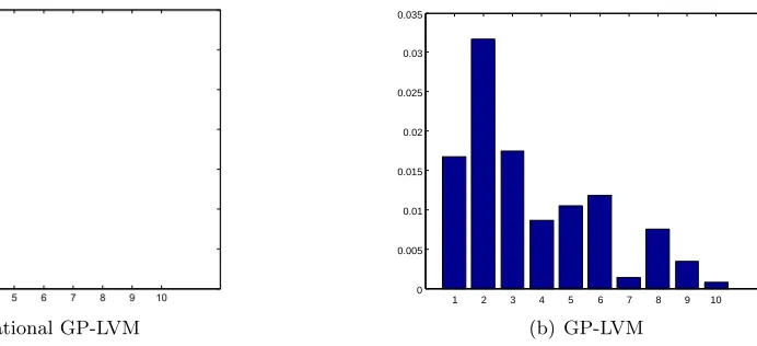
Figure 5: Left: The squared inverse lengthscales found by applying the variational GP-LVM with ARD EQ kernel on the oil flow data. Right: Results obtained for the standard GP-LVM with q = 10. These results demonstrate the ability of the variational GP-LVM to perform a “soft” automatic dimensionality selection. The inverse lengthscale for each dimension is associated with the expected number of the function’s upcrossings in that particular direction; small values denote a more linear behaviour, whereas values close to zero denote an irrelevant dimension. For the variational GP-LVM, plot (a) suggests that the non-linearity is captured by dimension 2, as also confirmed by plot 6(a). On the other hand, plot (b) demonstrates the overfitting problem of the GP-LVM which is trained with MAP.
5.2 Visualisation Tasks
Given a dataset with known structure, we can apply our algorithm and evaluate its per-formance in a simple and intuitive way, by checking if the form of the discovered low dimensional manifold agrees with our prior knowledge.
−3 −2 −1 0 1 2 −2
−1.5 −1 −0.5 0 0.5 1 1.5
(a) Variational GP-LVM,q= 10 (2D projection) −2 −1 0 1 2
−2 −1.5 −1 −0.5 0 0.5 1 1.5
(b) GP-LVM,q= 2
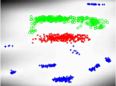
Figure 6: Panel 6(a) shows the means of the variational posterior q(X) for the variational GP-LVM, projected on the two dominant latent dimensions: dimension 2, plotted on they-axis, and dimension 3 plotted on thex-axis. The plotted projection of a latent pointxi,: is assigned a colour according to the label of the corresponding
output vectorxi,:. The greyscale background intensities are proportional to the
predicted variance of the GP mapping, if the corresponding locations were given as inputs. Plot 6(b) shows the visualisation found by standard sparse GP-LVM initialised with a two dimensional latent space.
GP-LVM are initialised based on PCA. Note that if we were to run the standard GP-LVM with 10 latent dimensions, the model would overfit the data and it would not reduce the dimensionality in the manner achieved by the variational GP-LVM, as illustrated in Figure 5(b). The quality of the class separation in the two-dimensional space can also be quantified in terms of the nearest neighbour error; the total error equals the number of training points whose closest neighbour in the latent space corresponds to a data point of a different class (phase of oil flow). The number of nearest neighbour errors made when finding the latent embedding for the variational GP-LVM is one. For the standard sparse GP-LVM it is 26, for the full GP-LVM with ARD kernel it is 8 and for the full GP-LVM with EQ kernel it is 2. Notice that all standard GP-LVMs were given the true dimensionality (q= 2) a priori.
5.3 Human Motion Capture Data
of 84 frames each. Our model does not require explicit timestamp information, since we know a priori that there is a constant time delay between poses and the model can construct equivalent covariance matrices given any vector of equidistant time points.
The model is jointly trained, as explained in the last paragraph of Section 3.3.2, on both walks and runs, i.e. the algorithm learns a common latent space for these motions. As in (Lawrence, 2007), we used 100 inducing points. At test time we investigate the ability of the model to reconstruct test data from a previously unseen sequence given partial information for the test targets. This is tested once by providing only the dimensions which correspond to the body of the subject and once by providing those that correspond to the legs. We compare with results in (Lawrence, 2007), which used MAP approximations for the dynamical models, and against nearest neighbour. We can also indirectly compare with the binary latent variable model (BLV) of Taylor et al. (2007) which used a slightly different data preprocessing. Furthermore, we additionally tested the non-dynamical version of our model, in order to explore the structure of the distribution found for the latent space. In this case, the notion of sequences or sub-motions is not modelled explicitly, as the non-dynamical approach does not model correlations between datapoints. However, as will be shown below, the model manages to discover the dynamical nature of the data and this is reflected in both, the structure of the latent space and the results obtained on test data.
The performance of each method is assessed by using the cumulative error per joint in the scaled space defined in (Taylor et al., 2007) and by the root mean square error in the angle space suggested by Lawrence (2007). Our models were initialised with nine latent dimensions. For the dynamical version, we performed two runs, once using the Mat´ern covariance function for the dynamical prior and once using the exponentiated quadratic.
The appropriate latent space dimensionality for the data was automatically inferred by our models. The non-dynamical model selected a 5-dimensional latent space. The model which employed the Mat´ern covariance to govern the dynamics retained four dimensions, whereas the model that used the exponentiated quadratic kept only three. The other latent dimensions were completely switched off by the ARD parameters.
Data CL CB L L B B
Error Type SC SC SC RA SC RA
BLV 11.7 8.8 - - -
-NN sc. 22.2 20.5 - - -
-GP-LVM (q= 3) - - 11.4 3.40 16.9 2.49
GP-LVM (q= 4) - - 9.7 3.38 20.7 2.72
GP-LVM (q= 5) - - 13.4 4.25 23.4 2.78
NN sc. - - 13.5 4.44 20.8 2.62
NN - - 14.0 4.11 30.9 3.20
VGP-LVM - - 14.22 5.09 18.79 2.79
Dyn. VGP-LVM (Exp. Quadr.) - - 7.76 3.28 11.95 1.90
Dyn. VGP-LVM (Mat´ern 3/2) - - 6.84 2.94 13.93 2.24
−4 −2 0 2
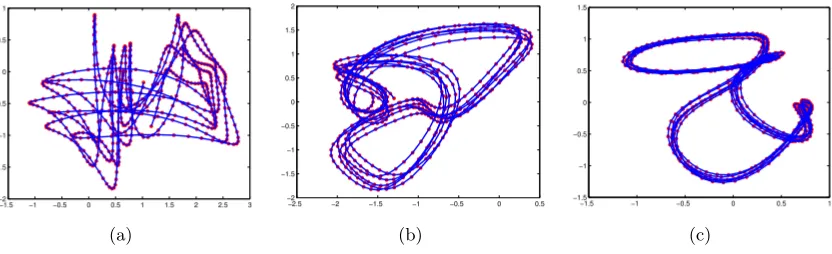
4 2 0 −2 −4 4 6 −5 −4 −3 −2 −1 0 1 2 3 (a) −4 −2 0 2 4 −6 −4 −2 0 2 4 −5 0 5 10 15 (b) −10 −5 0 5 −6 −4 −2 0 2 4 6 8 −10 −5 0 5 10 15 (c)
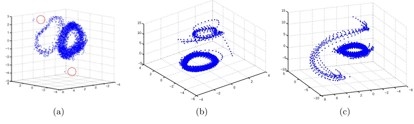
Figure 7: The latent space discovered by our models for the human motion capture data, projected into its three principal dimensions. The latent space found by the non-dynamical variational GP-LVM is shown in (a), by the non-dynamical model which uses the Mat´ern in (b) and by the dynamical model which uses the exponentiated quadratic in (c). The red, dotted circles highlight three “outliers”.
encoding for the “walk” and “run” regimes into two subspaces. Further, we notice that the smoother the latent space is constrained to be, the less “circular” is the shape of the “run” regime latent space encoding. This can be explained by noticing the “outliers” in the top left and bottom positions of plot (a), highlighted with a red, dotted circle. These latent points correspond to training positions that are very dissimilar to the rest of the training set but, nevertheless, a temporally constrained model is forced to accommodate them in a smooth path. The above intuitions can be confirmed by interacting with the model in real time graphically, as is presented in the supplementary video.
5.4 Modeling Raw High Dimensional Video Sequences
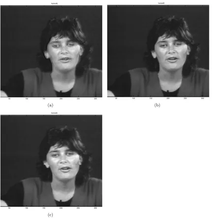
For this set of experiments we considered video sequences (which are included in the supple-mentary videos available on-line). Such sequences are typically preprocessed before mod-elling to extract informative features and reduce the dimensionality of the problem. Here we work directly with the raw pixel values to demonstrate the ability of the dynamical variational GP-LVM to model data with a vast number of features. This also allows us to directly sample video from the learned model.
Firstly, we used the model to reconstruct partially observed frames from test video se-quences.3 For the first video discussed here we gave as partial information approximately 50% of the pixels while for the other two we gave approximately 40% of the pixels on each frame. The mean squared error per pixel was measured to compare with the k−nearest neighbour (NN) method, for k ∈ (1, ..,5) (we only present the error achieved for the best choice of k in each case). The datasets considered are the following: firstly, the ‘Missa’ dataset, a standard benchmark used in image processing. This is a 103680-dimensional