DSA: Decentralized Double Stochastic
Averaging Gradient Algorithm
Aryan Mokhtari [email protected]
Alejandro Ribeiro [email protected]
Department of Electrical and Systems Engineering University of Pennsylvania
Philadelphia, PA 19104, USA
Editor:Mark Schmidt
Abstract
This paper considers optimization problems where nodes of a network have access to summands of a global objective. Each of these local objectives is further assumed to be an average of a finite set of functions. The motivation for this setup is to solve large scale machine learning problems where elements of the training set are distributed to multiple computational elements. The decentralized double stochastic averaging gradient (DSA) algorithm is proposed as a solution alternative that relies on: (i) The use of local stochastic averaging gradients. (ii) Determination of descent steps as differences of consecutive stochastic averaging gradients. Strong convexity of local functions and Lipschitz continuity of local gradients is shown to guarantee linear convergence of the sequence generated by DSA in expectation. Local iterates are further shown to approach the optimal argument for almost all realizations. The expected linear convergence of DSA is in contrast to the sublinear rate characteristic of existing methods for decentralized stochastic optimization. Numerical experiments on a logistic regression problem illustrate reductions in convergence time and number of feature vectors processed until convergence relative to these other alternatives. Keywords: decentralized optimization, stochastic optimization, stochastic averaging gradient, linear convergence, large-scale optimization, logistic regression
1. Introduction
We consider machine learning problems with large training sets that are distributed into a network of computing agents so that each of the nodes maintains a moderate number of samples. This leads to decentralized consensus optimization problems where summands of the global objective function are available at different nodes of the network. In this class of problems agents (nodes) try to optimize the global cost function by operating on their local functions and communicating with their neighbors only. Specifically, consider a variable x ∈ Rp and a connected network of size N where each nodenhas access to a local objective functionfn :Rp→R. The local objective function
fn(x) is defined as the average of qn local instantaneous functionsfn,i(x) that can be individually evaluated at noden. Agents cooperate to solve the global optimization problem
˜
x∗:= argmin
x
N X
n=1
fn(x) = argmin
x
N X
n=1
1
qn qn X
i=1
fn,i(x). (1)
The formulation in (1) models a training set with a total of PN
n=1qn training samples that are distributed among theNagents for parallel processing conducive to the determination of the optimal classifier ˜x∗ (Bekkerman et al. (2011); Tsianos et al. (2012a); Cevher et al. (2014)). Although we make no formal assumption, in cases of practical importance the total number of training samples PN
Analogous formulations are also of interest in decentralized control systems (Bullo et al. (2009); Cao et al. (2013); Lopes and Sayed (2008)), wireless systems (Ribeiro (2010, 2012)), and sensor networks (Schizas et al. (2008); Khan et al. (2010); Rabbat and Nowak (2004)). Our interest here is in solving (1) with a method that has the following three properties
• Decentralized; nodes operate on their local functions and communicate with neighbors only.
• Stochastic; nodes determine a descent direction by evaluating only one out of theqn functions
fn,i at each iteration.
• Linear convergence rate; the expected distance to the optimum is scaled by a subunit factor at each iteration.
Decentralized optimization is relatively mature and various methods are known with complemen-tary advantages. These methods include decentralized gradient descent (DGD) (Nedi´c and Ozdaglar (2009); Jakovetic et al. (2014); Yuan et al. (2013)), network Newton (Mokhtari et al. (2015a,b)), decentralized dual averaging (Duchi et al. (2012); Tsianos et al. (2012b)), the exact first order al-gorithm (EXTRA) (Shi et al. (2015)), as well as the alternating direction method of multipliers (ADMM) (Boyd et al. (2011); Schizas et al. (2008); Shi et al. (2014); Iutzeler et al. (2013)) and its linearized variants (Ling and Ribeiro (2014); Ling et al. (2015); Mokhtari et al. (2015c)). The ADMM, its variants, and EXTRA converge linearly to the optimal argument but DGD, network Newton, and decentralized dual averaging have sublinear convergence rates. Of particular impor-tance to this paper, is the fact that DGD has (inexact) linear convergence to a neighborhood of the optimal argument when it uses constant stepsizes. It can achieve exact convergence by using dimin-ishing stepsizes, but the convergence rate degrades to sublinear. This lack of linear convergence is solved by EXTRA through the use of iterations that rely on information of two consecutive steps (Shi et al. (2015)).
All of the algorithms mentioned above require the computationally costly evaluation of the local gradients ∇fn(x) = (1/qn)P
qn
i=1∇fn,i(x). This cost can be avoided by stochastic decentralized algorithms that reduce computational cost of iterations by substituting all local gradients with their stochastic approximations. This reduces the computational cost per iteration but results in sublinear convergence rates of order O(1/t) even if the corresponding deterministic algorithm exhibits linear convergence. This is a drawback that also exists in centralized stochastic optimization where linear convergence rates in expectation are established by decreasing the variance of the stochastic gradient approximation (Roux et al. (2012); Schmidt et al. (2013); Shalev-Shwartz and Zhang (2013); Johnson and Zhang (2013); Koneˇcn`y and Richt´arik (2013); Defazio et al. (2014)). In this paper we build on the ideas of the stochastic averaging gradient (SAG) algorithm (Schmidt et al. (2013)) and its unbiased version SAGA (Defazio et al. (2014)). Both of these algorithms use the idea of stochastic incremental averaging gradients. At each iteration only one of the stochastic gradients is updated and the average of all of the most recent stochastic gradients is used for estimating the gradient.
The contribution of this paper is to develop the decentralized double stochastic averaging gradient (DSA) method, a novel decentralized stochastic algorithm for solving (1). The method exploits a new interpretation of EXTRA as a saddle point method and uses stochastic averaging gradients in lieu of gradients. DSA isdecentralized because it is implementable in a network setting where nodes can communicate only with their neighbors. It isdoublebecause iterations utilize the information of two consecutive iterates. It isstochasticbecause the gradient of only one randomly selected function is evaluated at each iteration and it is anaveraging method because it uses an average of stochastic gradients to approximate the local gradients. DSA is proven to converge linearly to the optimal argument ˜x∗ in expectation when the local instantaneous functions fn,i are strongly convex, with Lipschitz continuous gradients. This is in contrast to all other decentralized stochastic methods to solve (1) that converge at sublinear rates.
by stochastic averaging gradients (Section 2). We follow with a digression on the limit points of DGD and EXTRA iterations to explain the reason why DGD does not achieve exact convergence but EXTRA is expected to do so (Section 2.1). A reinterpretation of EXTRA as a saddle point method that solves for the critical points of the augmented Lagrangian of a constrained optimization problem equivalent to (1) is then introduced. It follows from this reinterpretation that DSA is a stochastic saddle point method (Section 2.2). The fact that DSA is a stochastic saddle point method is the critical enabler of the subsequent convergence analysis (Section 3). In particular, it is possible to guarantee that strong convexity and gradient Lipschitz continuity of the local instantaneous functions fn,i imply that a Lyapunov function associated with the sequence of iterates generated by DSA converges linearly to its optimal value in expectation (Theorem 7). Linear convergence in expectation of the local iterates to the optimal argument ˜x∗ of (1) follows as a trivial consequence (Corollary 8). We complement this result by showing convergence of all the local variables to the optimal argument ˜x∗ with probability 1 (Theorem 9).
The advantages of DSA relative to a group of stochastic and deterministic alternatives in solving a logistic regression problem are then studied in numerical experiments (Section 4). These results demonstrate that DSA is the only decentralized stochastic algorithm that reaches the optimal solu-tion with a linear convergence rate. We further show that DSA outperforms deterministic algorithms when the metric is the number of times that elements of the training set are evaluated. The behavior of DSA for different network topologies is also evaluated. We close the paper with pertinent remarks (Section 5).
Notation Lowercase boldfacevdenotes a vector and uppercase boldfaceAa matrix. For column vectorsx1, . . . ,xN we use the notationx= [x1;. . .;xN] to represent the stack column vectorx. We usekvkto denote the Euclidean norm of vectorvandkAkto denote the Euclidean norm of matrixA. For a vectorvand a positive definite matrixA, theA-weighted norm is defined askvkA:=
√ vTAv. The null space of matrixAis denoted by null(A) and the span of a vector by span(x). The operator
Ex[·] stands for expectation over random variable x and E[·] for expectation with respect to the
distribution of a stochastic process.
2. Decentralized Double Stochastic Averaging Gradient
Consider a connected network that containsN nodes such that each nodencan only communicate with peers in its neighborhood Nn. Define xn ∈Rp as a local copy of the variable x that is kept
at noden. In decentralized optimization, agents try to minimize their local functionsfn(xn) while ensuring that their local variablesxncoincide with the variablesxmof all neighborsm∈ Nn– which, given that the network is connected, ensures that the variables xn of all nodes are the same and renders the problem equivalent to (1). DGD is a well known method for decentralized optimization that relies on the introduction of nonnegative weightswij≥0 that are not null if and only ifm=n or ifm∈ Nn. Lettingt∈Nbe a discrete time index andαa given stepsize, DGD is defined by the
recursion
xtn+1= N X
m=1
wnmxtm−α∇fn(xtn), n= 1, . . . , N. (2)
Sincewnm= 0 whenm6=nandm /∈ Nn, it follows from (2) that nodenupdatesxn by performing an average over the variablesxt
mof its neighborsm∈ Nnand its ownxtn, followed by descent through the negative local gradient −∇fn(xtn). If a constant stepsize is used, DGD iterates xtn approach a neighborhood of the optimal argument ˜x∗ of (1) but don’t converge exactly. To achieve exact convergence diminishing stepsizes are used but the resulting convergence rate is sublinear (Nedi´c and Ozdaglar (2009)).
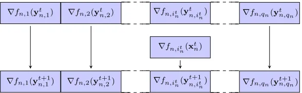
∇fn,1(yt
n,1) ∇fn,2(ytn,2) ∇fn,it n(y
t n,it
n) ∇fn,qn(y t n,qn)
∇fn,it n(x
t n)
∇fn,1(yn,1t+1) ∇fn,2(y t+1
n,2) ∇fn,it
n(y t+1 n,it n
) ∇fn,qn(y
t+1 n,qn)
Figure 1: Stochastic averaging gradient table at noden. At each iterationta random local instanta-neous gradient∇fn,it
n(y
t n,it
n) is updated by∇fn,i t n(x
t
n). The rest of the local instantaneous gradients remain unchanged, i.e., ∇fn,i(yn,it+1) =∇fn,i(yn,it ) for i6=itn. This list is used to compute the stochastic averaging gradient in (7).
˜
wnmwith the same properties as the weightswnm and define EXTRA through the recursion
xtn+1=xtn+ N X
m=1
wnmxtm− N X
m=1
˜
wnmxtm−1−α
∇fn(xtn)− ∇fn(xtn−1)
, n= 1, . . . , N. (3)
Observe that (3) is well defined fort >0. Fort= 0 we utilize the regular DGD iteration in (2). In the nomenclature of this paper we say that EXTRA performs a decentralized double gradient descent step because it operates in a decentralized manner while utilizing a difference of two gradients as descent direction. Minor modification as it is, the use of this gradient difference in lieu of simple gradients, endows EXTRA with exact linear convergence to the optimal argument ˜x∗ under mild assumptions (Shi et al. (2015)).
If we recall the definitions of the local functions fn(xn) and the instantaneous local functions
fn,i(xn) available at node n, the implementation of EXTRA requires that each node ncomputes the full gradient of its local objective functionfn atxtn as
∇fn(xtn) = 1
qn qn X
i=1
∇fn,i(xtn). (4)
This is computationally expensive when the number of instantaneous functionsqnis large. To resolve this issue, local stochastic gradients can be substituted for the local objective functions gradients in (3). These stochastic gradients approximate the gradient∇fn(xn) of nodenby randomly choosing one of the instantaneous functions gradients∇fn,i(xn). If we letitn∈ {1, . . . qn} denote a function index that we choose at timet at nodenuniformly at random and independently of the history of the process, then the stochastic gradient is defined as
ˆ
sn(xtn) :=∇fn,it n(x
t
n). (5)
We can then write a stochastic version of EXTRA by replacing∇fn(xtn) by ˆsn(xtn) and∇fn(xtn−1) by ˆ
sn(xtn−1). Such an algorithm would have a small computational cost per iteration. On the negative side, it either has a linear convergence to a neighborhood of the optimal solutionx∗ with constant stepsizeα, or it would converge sublinearly to the optimal argument when the stepisize diminishes as time passes. Here however, we want to design an algorithm with low computational complexity that converges linearly to the exact solutionx∗.
list for gradient approximation; see Figure 1. Formally, define the variableyn,i ∈Rp to represent
the iterate value the last time that the instantaneous gradient of function fn,i was evaluated. If we letitn ∈ {1, . . . , qn} denote the function index chosen at time t at noden, as we did in (5), the variablesyn,i are updated recursively as
yn,it+1=xtn, ifi=itn, yn,it+1=ytn,i, ifi6=itn. (6) With these definitions in hand we can define the stochastic averaging gradient at nodenas
ˆ
gtn:=∇fn,it n(x
t
n)− ∇fn,it n(y
t n,it
n) + 1
qn qn X
i=1
∇fn,i(ytn,i). (7)
Observe that to implement (7) the gradients∇fn,i(ytn,i) are stored in the local gradient table shown in Figure 1.
The DSA algorithm is a variation of EXTRA that substitutes the local gradients∇fn(xtn) in (3) for the local stochastic average gradients ˆgtn in (7),
xtn+1=xtn+ N X
m=1
wnmxtm− N X
m=1
˜
wnmxtm−1−α
ˆ
gtn−gˆtn−1. (8)
The DSA initial update is given by applying the same substitution for the update of DGD in (2) as
x1n= N X
m=1
wnmx0m−αˆg
0
n. (9)
DSA is summarized in Algorithm 1 for t ≥ 0. The DSA update in (8) is implemented in Step 9. This step requires access to the local iterates xt
m of neighboring nodes m ∈ Nn which are collected in Step 2. Furthermore, implementation of the DSA update also requires access to the stochastic averaging gradients ˆgt−1
n and ˆgnt. The latter is computed in Step 4 and the former is computed and stored at the same step in the previous iteration. The computation of the stochastic averaging gradients requires the selection of the indexit
n. This index is chosen uniformly at random in Step 3. Determination of stochastic averaging gradients also necessitates access and maintenance of the gradients table in Figure 1. The it
n element of this table is updated in Step 5 by replacing ∇fn,it
n(y
t n,it
n) with∇fn,i t n(x
t
n), while the other vectors remain unchanged. To implement the first DSA iteration at timet = 0 we have to perform the update in (9) instead of the update in (8) as in Step 7. Further observe that the auxiliary variables y0
n,i are initialized to the initial iterate x0n. This implies that the initial values of the stored gradients are∇fn,i(yn,i0 ) =∇fn,i(x0n).
We point out that the weightswnm and ˜wnm can’t be arbitrary. If we define weight matricesW and ˜W with elements wnm and ˜wnm, respectively, they have to satisfy conditions that we state as an assumption for future reference.
Assumption 1 The weight matricesW andW˜ must satisfy the following properties
(a) Both are symmetric, W=WT andW˜ = ˜WT.
(b) The null space of I−W˜ includes the span of1, i.e., null(I−W)˜ ⊇span(1), the null space of
I−Wis the span of1, i.e., null(I−W) =span(1), and the null space of the differenceW˜ −W
is the span of 1, i.e., null( ˜W−W) =span(1).
Algorithm 1DSA algorithm at noden
Require: Vectorsx0
n. Gradient table initialized with instantaneous gradients∇fn,i(y0n,i) withy0n,i=x0n. 1: fort= 0,1,2, . . .do
2: Exchange variablext
nwith neighboring nodesm∈ Nn; 3: Chooseitnuniformly at random from the set{1, . . . , qn}; 4: Compute and store stochastic averaging gradient as per (7):
ˆ
gtn=∇fn,it n(x
t
n)− ∇fn,it n(y
t n,it
n) +
1 qn
qn
X
i=1
∇fn,i(ytn,i);
5: Takeyn,it+1t n=x
t
nand store∇fn,it n(y
t+1 n,it
n) =∇fn,i t n(x
t n) ini
t
ngradient table position. All other entries
in the table remain unchanged. The vectoryt+1n,it
nis not explicitly stored;
6: if t= 0then
7: Update variablextn as per (9): x t+1
n =
N
X
m=1
wnmxtn−αˆg t n;
8: else
9: Update variablext
n as per (8): x t+1
n =x
t
n+
N
X
m=1
wnmxtn− N
X
m=1
˜ wnmxt
−1
n −α
ˆ gtn−ˆg
t−1 n
;
10: end if
11: end for
Requiring the matrixWto be symmetric and with specific null space properties is necessary to let all agents converge to the same optimal variable. Analogous properties are necessary in DGD and are not difficult to satisfy. The condition on spectral ordering is specific to EXTRA but is not difficult to satisfy either. E.g., if we have a matrixWthat satisfies all the conditions in Assumption 1, the weight matrix ˜W= (I+W)/2 makes Assumption 1 valid.
We also point that, as written in (7), computation of local stochastic averaging gradients ˆgt n is costly because it requires evaluation of the sumPqn
i=1∇fn,i(ytn,i) at each iteration. To be more precise, if we implement the update in (7) naively, at each iteration we should compute the sum Pqn
i=1∇fn,i(ytn,i) which has a computational cost of the orderO(qn). This cost can be avoided by updating the sum at each iteration with the recursive formula
qn X
i=1
∇fn,i(ytn,i) = qn X
i=1
∇fn,i(ytn,i−1) +∇fn,it−1n (x
t−1
n )− ∇fn,it−1n (y
t−1
n,it−1n
). (10)
Using the update in (10), we can update the sumPqn
i=1∇fn,i(ytn,i) required for (7) in a computation-ally efficient manner. Important properties and interpretations of EXTRA and DSA are presented in the following sections after pertinent remarks.
Remark 1 The local stochastic averaging gradients in (7) are unbiased estimates of the local gra-dients ∇fn(xtn). Indeed, if we let Ft measure the history of the system up until time t we have that the sum in (7) is deterministic given this sigma-algebra. This observation implies that the con-ditional expectation E(1/qn)P
qn
i=1∇fn,i(ytn,i)| F t
can be simplified as (1/qn)P qn
i=1∇fn,i(ytn,i). Thus, the conditional expectation of the stochastic averaging gradient is,
Egˆtn Ft
=E
h ∇fn,it
n(x t n) Ft i −E h ∇fn,it
n(y t n,it n) Ft i + 1 qn qn X i=1
∇fn,i(ytn,i). (11)
With the indexit
n chosen equiprobably from the set{1, . . . , qn}, the expectation of the second term in (11) is the same as the sum in the last term – each of the indexes is chosen with probability
1/qn. In other words, we can write E
h ∇fn,it
n(y t n,it n) Ft i
= (1/qn)P qn
these two terms cancel out each other and, since the expectation of the first term in (11) is simply
E∇fn,it n(x
t n)
Ft
= (1/qn)P qn
i=1∇fn,i(xtn) =∇fn(xtn), we can simplify (11) to
Eˆgnt Ft
=∇fn(xtn). (12)
The expression in (12) means, by definition, that ˆgt
n is an unbiased estimate of∇fn(xtn) when the historyFtis given.
Remark 2 The local stochastic averaging gradient ˆgtnat nodencontains three terms. The first two terms∇fn,it
n(x
t
n) and∇fn,it n(y
t n,it
n) are the new and old gradients of the chosen objective function fn,it
n at noden, respectively. The last term (1/qn) Pqn
i=1∇fn,i(ytn,i) is the average of the average of all the instantaneous gradients available at node n. This update can be considered as a localized version of the stochastic averaging gradient update in the SAGA algorithm (Defazio et al. (2014)). Notice that instead of the difference∇fn,it
n(x
t
n)− ∇fn,it n(y
t n,it
n) in (7) we could use the difference (∇fn,it
n(x
t
n)− ∇fn,it n(y
t n,it
n))/qn which would lead to stochastic averaging gradient suggested in the SAG algorithm (Schmidt et al. (2013)). As studied in (Defazio et al. (2014)), both of these approximations lead to a variance reduction method. The one suggested by SAGA is an unbiased estimator of the exact gradient (1/qn)P
qn
i=1∇fn,i(xtn), while the one suggested by SAG is a biased estimator of the gradient with smaller variance. Since the analysis of the estimator suggested by SAGA is simpler, we use its idea to define the local stochastic averaging gradient ˆgt
n in (7).
2.1 Limit Points of DGD and EXTRA
The derivation of EXTRA hinges on the observation that the optimal argument of (1) is not a fixed point of the DGD iteration in (2) but is a fixed point of the iteration in (3). To explain this point define x := [x1;. . .;xN] ∈ RN p as a vector that concatenates the local iterates xn and the aggregate functionf :RN p→Ras the one that takes valuesf(x) =f(x1, . . . ,xN) :=P
N
n=1fn(xn). Decentralized optimization entails the minimization off(x) subject to the constraint that all local variables are equal,
x∗:= argminf(x) =f(x1, . . . ,xN) = N X
n=1
fn(xn),
s.t. xn=xm, for alln, m. (13)
The problems in (1) and (13) are equivalent in the sense that the vectorx∗ ∈RN p is a solution of
(13) if it satisfies x∗n = ˜x∗ for all n, or, equivalently, if we can writex∗ = [˜x∗;. . .; ˜x∗]. Regardless of interpretation, the Karush, Kuhn, Tucker (KKT) conditions of (13) dictate that that optimal argumentx∗ must sastisfy
x∗⊂span(1N ⊗Ip), (1N ⊗Ip)T∇f(x∗) =0. (14)
The first condition in (14) requires that all the local variablesx∗nbe equal, while the second condition requires the sum of local gradients to vanish at the optimal point. This latter condition is not the same as∇f(x) =0. If we observe that the gradient∇f(xt) of the aggregate function can be written as ∇f(x) = [∇f1(x1);. . .;∇fN(xN)] ∈ RN p, the condition ∇f(x) = 0 implies that all the local
gradients are null, i.e., that ∇fn(xn) =0 for all n. This is stronger than having their sum being null as required by (14).
Define now the extended weight matrices as the Kronecker products Z := W⊗I ∈ RN p×N p and ˜Z := ˜W⊗I ∈ RN p×N p. Note that the required conditions for the weight matrices W and
˜
Assumption 1(b) imply that null{Z−Z}˜ = span{1⊗I}, null{I−Z}= span{1⊗I}, and null{I−Z} ⊇˜ span{1⊗I}. Lastly, the spectral properties of matrices Wand ˜W in Assumption 1(c) yield that matrix ˜Zis positive definite and the expressionZZ˜ (I+Z)/2 holds.
According to the definition of the extended weight matrixZ, the DGD iteration in (2) is equivalent to
xt+1=Zxt−α∇f(xt), (15)
where, according to (13), the gradient∇f(xt) of the aggregate function can be written as∇f(xt) = [∇f1(xt1);. . .;∇fN(xtN)]∈R
N p. Likewise, the EXTRA iteration in (3) can be written as
xt+1= (I+Z)xt−Zx˜ t−1−α∇f(xt)− ∇f(xt−1). (16) The fundamental difference between DGD and EXTRA is that a fixed point of (15) does not nec-essarily satisfy (14), whereas the fixed points of (16) are guaranteed to do so. Indeed, taking limits in (15) we see that the fixed pointsx∞ of DGD must satisfy
(I−Z)x∞+α∇f(x∞) =0, (17)
which is incompatible with (14) except in peculiar circumstances – such as, e.g., when all local functions have the same minimum. The limit points of EXTRA, however, satisfy the relationship
x∞−x∞= (Z−Z)x˜ ∞−α[∇f(x∞)− ∇f(x∞)]. (18)
Canceling out the variables on the left hand side and the gradients in the right hand side it follows that (Z−Z)x˜ ∞=0. Since the null space of ofZ−Z˜ is null(Z−Z) =˜ 1N ⊗Ip by assumption, we must havex∞⊂span(1N⊗Ip). This is the first condition in (14). For the second condition in (14) sum the updates in (16) recursively and use the telescopic nature of the sum to write
xt+1= ˜Zxt−α∇f(xt)− t X
s=0
( ˜Z−Z)xs. (19)
Substituting the limit point in (19) and reordering terms, we see thatx∞ must satisfy
α∇f(x∞) = (I−Z)x˜ ∞−
∞
X
s=0
( ˜Z−Z)xs. (20)
In (20) we have that (I−Z)x˜ ∞ =0 because the null space of (I−Z) is null(Z˜ −Z) =˜ 1N ⊗Ip by assumption and x∞ ⊂ span(1N ⊗Ip) as already shown. Implementing this simplification and considering the multiplication of the resulting equality by (1N ⊗Ip)T we obtain
(1N⊗Ip)Tα∇f(x∞) =−
∞
X
s=0
(1N ⊗Ip)T(Z−Z)x˜ s. (21)
In (21), the terms (1N⊗Ip)T(Z−Z) =˜ 0because the matricesZand ˜Zare symmetric and (1N⊗Ip) is in the null space of the difference Z−Z. This implies that (1˜ N ⊗Ip)Tα∇f(x∞) =0, which is the second condition in (14). Therefore, given the assumption that the sequence of EXTRA iterates xthas a limit pointx∞ it follows that this limit point satisfies both conditions in (14) and for this
reason exact convergence with constant stepsize is achievable for EXTRA.
2.2 Stochastic Saddle Point Method Interpretation of DSA
vectorsvt=Pt
s=0( ˜Z−Z)1/2xs. The vectorvtrepresents the accumulation of variable dissimilarities
in different nodes over time. Considering this definition ofvt we can rewrite (19) as
xt+1=xt−α
∇f(xt) + 1
α(I−
˜ Z)xt+ 1
α( ˜Z−Z)
1/2vt
. (22)
Furthermore, based on the definition of the sequence vt = Pt
s=0( ˜Z−Z)
1/2xs we can write the recursive expression
vt+1=vt+α
1
α( ˜Z−Z)
1/2
xt+1
. (23)
Consider x as a primal variable andv as a dual variable. Then, the updates in (22) and (23) are equivalent to the updates of a saddle point method with stepsizeαthat solves for the critical points of the augmented Lagrangian
L(x,v) =f(x) + 1
αv
T( ˜Z−Z)1/2x+ 1
2αx
T(I−Z)x˜ . (24)
In the Lagrangian in (24) the factor (1/α)vT( ˜Z−Z)1/2x stems from the linear constraint ( ˜Z−
Z)1/2x=0and the quadratic term (1/2α)xT(I−Z)x˜ is the augmented term added to the Lagrangian. Therefore, the optimization problem whose augmented Lagrangian is the one given in (24) is
x∗= argmin
x
f(x) s.t. 1
α( ˜Z−Z)
1/2x=0. (25)
Observing that the null space of ( ˜Z−Z)1/2 is null(( ˜Z−Z)1/2) = null( ˜Z−Z) = span{1
N ⊗Ip}, the constraint in (25) is equivalent to the consensus constraint xn =xm for all n, m that appears in (13). This means that (25) is equivalent to (13), which, as already argued, is equivalent to the original problem in (1). Hence, EXTRA is a saddle point method that solves (25) which, because of their equivalence, is tantamount to solving (1). Considering that saddle point methods converge linearly, it follows that the same is true of EXTRA.
That EXTRA is a saddle point method provides a simple explanation of its convergence prop-erties. For the purposes of this paper, however, the important fact is that if EXTRA is a sad-dle point method, DSA is a stochastic sadsad-dle point method. To write DSA in this form define ˆ
gt:= [ˆgt
1;. . .; ˆgNt ]∈R
N pas the vector that concatenates all the local stochastic averaging gradients
at stept. Then, the DSA update in (8) can be written as
xt+1= (I+Z)xt−Zx˜ t−1−α ˆ
gt−gˆt−1
. (26)
Comparing (16) and (26) we see that they differ in the latter using stochastic averaging gradients ˆ
gtin lieu of the full gradients∇f(xt). Therefore, DSA is a stochastic saddle point method in which the primal variables are updated as
xt+1=xt−αˆgt−(I−Z)x˜ t−( ˜Z−Z)1/2vt, (27) and the dual variablesvt are updated as
vt+1=vt+ ( ˜Z−Z)1/2xt+1. (28) Notice that the initial primal variable x0 is an arbitrary vector in
RN p, while according to the
definitionvt=Pt
s=0( ˜Z−Z)
1/2xs. We then need to set the initial multiplier tov0= ( ˜Z−Z)1/2x0.
3. Convergence Analysis
Our goal here is to show that as time progresses the sequence of iteratesxtapproaches the optimal argumentx∗. To do so, in addition to the conditions on the weight matricesWand ˜Win Assumption 1, we assume the instantaneous local functionsfn,i have specific properties that we state next.
Assumption 2 The instantaneous local functions fn,i(xn) are differentiable and strongly convex with parameterµ.
Assumption 3 The gradient of instantaneous local functions ∇fn,i are Lipschitz continuous with parameterL, i.e., for alln∈ {1, . . . , N}andi∈ {1, . . . , qn}we can write
k∇fn,i(a)− ∇fn,i(b)k ≤Lka−bk a,b∈Rp. (29)
The condition imposed by Assumption 2 implies that the local functionsfn(xn) and the global cost functionf(x) = PN
n=1fn(xn) are also strongly convex with parameterµ. Likewise, Lipschitz continuity of the local instantaneous gradients considered in Assumption 3 enforces Lipschitz conti-nuity of the local functions gradient∇fn(xn) and the aggregate function gradient∇f(x) – see, e.g., (Lemma 1 of Mokhtari et al. (2015a)).
3.1 Preliminaries
In this section we study some basic properties of the sequences of primal and dual variables generated by the DSA algorithm. In the following lemma, we study the relation of the iteratesxtandvtwith the optimal primalx∗ and dualv∗ arguments.
Lemma 3 Consider the DSA algorithm as defined in (6)-(9)and recall the updates of the primalxt
and dualvtvariables in (27)and (28), respectively. Further, define the positive semidefinite matrix
U:= ( ˜Z−Z)1/2. If Assumption 1 holds true, then the sequence of primalxt and dualvtvariables satisfy
αgˆt− ∇f(x∗)= (I+Z−2 ˜Z)(x∗−xt+1) + ˜Z(xt−xt+1)−U(vt+1−v∗). (30) Proof Considering the update rule for the dual variable in (28) and the definitionU= ( ˜Z−Z)1/2,
we can substituteUvtin (27) byUvt+1−U2xt+1. Applying this substitution into the DSA primal
update in (27) yields
αgˆt=−(I+Z−Z)x˜ t+1+ ˜Zxt−Uvt+1. (31) By adding and subtracting ˜Zxt+1 to the right hand side of (31) and considering the fact that
(I+Z−2 ˜Z)x∗=0we obtain
αˆgt= (I+Z−2 ˜Z)(x∗−xt+1) + ˜Z(xt−xt+1)−Uvt+1. (32) One of the KKT conditions of problem (25) implies that the optimal variables x∗ and v∗ satisfy
α∇f(x∗) +Uv∗=0or equivalently−α∇f(x∗) =Uv∗. Adding this equality to both sides of (32) follows the claim in (30).
In the subsequent analyses of convergence of DSA, we need an upper bound for the expected value of squared difference between the stochastic averaging gradient ˆgtand the optimal argument gradient∇f(x∗) given the observations until stept, i.e. Ehkgˆt− ∇f(x∗)k2
| Fti. To establish this
upper bound first we define the sequencept∈
Ras
pt:= N X
n=1
1
qn qn X
i=1
fn,i(ytn,i)−fn,i(˜x∗)− ∇fn,i(˜x∗)T(yn,it −˜x
∗)
Notice that based on the strong convexity of the local instantaneous functions fn,i, each term
fn,i(ytn,i)−fn,i(˜x∗)− ∇fn,i(˜x∗)T(ytn,i−x˜∗) is positive and as a result the sequence p
t defined in
(33) is always positive. In the following lemma, we use the result in Lemma 3 to guarantee an upper bound for the expectation Ekˆgt− ∇f(x∗)k2| Ft in terms of pt and the optimality gap
f(xt)−f(x∗)− ∇f(x∗)T(xt−x∗).
Lemma 4 Consider the DSA algorithm in (6)-(9)and the definition of the sequence pt in (33). If
Assumptions 1-3 hold true, then the squared norm of the difference between the stochastic averaging
gradientgˆtand the optimal gradient ∇f(x∗)in expectation is bounded above by
E
h
ˆgt− ∇f(x∗)
2
| Fti≤4Lpt+ 2 (2L−µ) f(xt)−f(x∗)− ∇f(x∗)T(xt−x∗)
. (34)
Proof See Appendix A.
Observe that as the sequence of iterates xt approaches the optimal argument x∗, all the local auxiliary variables ytn,i converge to ˜x∗ which follows convergence of pt to null. This observation in association with the result in (34) implies that the expected value of the difference between the stochastic averaging gradient ˆgtand the optimal gradient∇f(x∗) vanishes as the sequence of iterates xtapproaches the optimal argument x∗.
3.2 Convergence
In this section we establish linear convergence of the sequence of iterates xt generated by DSA to the optimal argumentx∗. To do so, define 0< γand Γ<∞as the smallest and largest eigenvalues of the positive definite matrix ˜Z, respectively. Likewise, defineγ0as the smallest non-zero eigenvalue
of the matrix ˜Z−Zand Γ0 as the largest eigenvalue of the matrix ˜Z−Z. Further, define the vectors
ut,u∗∈
R2N pand matrixG∈R2N p×2N pas
u∗:=
x∗ v∗
, ut:=
xt vt
, G=
˜
Z 0
0 I
. (35)
Observe that the vector u∗ ∈ R2N p concatenates the optimal primal and dual variables and the vector ut ∈
R2N p contains primal and dual iterates at stept. Further, G∈R2N p×2N p is a block
diagonal positive definite matrix that we introduce since instead of tracking the value of `2 norm
kut−u∗k2
2 we study the convergence properties ofGweighted normkut−u∗k2G. Notice that the
weighted norm kut−u∗k2
G is equivalent to (ut−u∗)TG(ut−u∗). Our goal is to show that the
sequencekut−u∗k2
Gconverges linearly to null. To do this we show linear convergence of a Lyapunov
function of the sequencekut−u∗k2
G. The Lyapunov function is defined askut−u∗k2G+cptwhere
c >0 is a positive constant.
To prove linear convergence of the sequencekut−u∗k2 G+cp
twe first show an upper bound for
the expected errorEkut+1−u∗k2G| F
t
in terms ofkut−u∗k2
Gand some parameters that capture
optimality gap.
Lemma 5 Consider the DSA algorithm as defined in (6)-(9). Further recall the definitions ofptin
(33)andut,u∗, andGin (35). If Assumptions 1-3 hold true, then for any positive constant η >0
we can write
Ekut+1−u∗k2G| F
t
≤ kut−u∗k2G−2E
h
kxt+1−x∗kI+Z−2 ˜2 Z| Fti+α4L
η p
t
−E
h
kxt+1−xtk2 ˜
Z−2αηI| F
ti−
Ekvt+1−vtk2| Ft
− 4αµ
L −
2α(2L−µ)
η
f(xt)−f(x∗)− ∇f(x∗)T(xt−x∗)
Proof See Appendix B.
Lemma 5 shows an upper bound for the squared norm kut+1−u∗k2
Gwhich is the first part of
the Lyapunov functionkut−u∗k2
G+cptat stept+ 1. Likewise, we provide an upper bound for the
second term of the Lyapunov function at timet+ 1 which ispt+1in terms ofptand some parameters that capture optimality gap. This bound is studied in the following lemma.
Lemma 6 Consider the DSA algorithm as defined in (6)-(9)and the definition ofptin (33).
Fur-ther, defineqminandqmaxas the smallest and largest values for the number of instantaneous functions
at a node, respectively. If Assumptions 1-3 hold true, then for allt >0 the sequenceptsatisfies
Ept+1| Ft≤
1− 1
qmax
pt+ 1
qmin
f(xt)−f(x∗)− ∇f(x∗)T(xt−x∗)
. (37)
Proof See Appendix C.
Lemma 6 provides an upper bound forpt+1 in terms of its previous valueptand the optimality errorf(xt)−f(x∗)− ∇f(x∗)T(xt−x∗). Combining the results in Lemmata 5 and 6 we can show
that in expectation the Lyapunov function kut+1−u∗k2
G+c pt+1 at stept+ 1 is strictly smaller
than its previous valuekut−u∗k2
G+c ptat stept.
Theorem 7 Consider the DSA algorithm as defined in (6)-(9). Further recall the definition of the
sequence pt in (33). Define η as an arbitrary positive constant chosen from the interval
η∈ L2q
max
µqmin
+L
2
µ −
L
2 , ∞
. (38)
If Assumptions 1-3 hold true and the stepsize αis chosen from the interval α∈(0, γ/2η), then for
arbitraryc chosen from the interval
c∈
4αLq
max
η ,
4αµqmin
L −
2αqmin(2L−µ)
η
, (39)
there exits a positive constant0< δ <1 such that
Ekut+1−u∗k2G+c p
t+1| Ft
≤(1−δ) kut−u∗k2 G+c p
t
. (40)
Proof See Appendix D.
We point out that the linear convergence constant δin (40) is explicitly available – see (100) in Appendix D. It is a function of the strong convexity parameterµ, the Lipschitz continuity constant
L, lower and upper bounds on the eigenvalues of the matrices ˜Z, ˜Z−Z, andI+Z−2 ˜Z, the smallest
qminand largestqmax values for the number of instantaneous functions available at a node, and the
stepsizeα. Insight on the dependence ofδwith problem parameters is offered in Section 3.3. The inequality in (40) shows that the expected value of the sequencekut−u∗k2
G+c p
t at time
t+ 1 given the observation until stept is strictly smaller than the previous iterate at step t. Note that, it is not hard to verify that if the positive constantη is chosen from the interval in (38), the interval in (39) is non-empty. Computing the expected value with respect to the initial sigma field
E.| F0 =E[.] implies that in expectation the sequence kut−u∗k2G+c pt converges linearly to
null, i.e.,
Ekut−u∗k2G+c p
t
≤(1−δ)t ku0−u∗k2 G+c p
0
. (41)
Corollary 8 Consider the DSA algorithm as defined in(6)-(9)and recallγis the minimum
eigen-value of the positive definite matrixZ˜. Suppose the conditions of Theorem 7 hold, then there exits a
positive constant0< δ <1 such that
Ekxt−x∗k2≤(1−δ)t
ku0−u∗k2 G+c p
0
.
γ (42)
Proof First note that according to the definitions of uand Gin (35) and the definition ofpt in (33) , we can writekxt−x∗k2
˜ Z≤ ku
t−u∗k2 G+c p
t. Further, note that the weighted normkxt−x∗k2 ˜ Z
is lower bounded byγkxt−x∗k2, sinceγis a lower bound for the eigenvalues of ˜Z. Combine these
two observations to obtain γkxt−x∗k2 ≤ kut−u∗k2 G+c p
t. This inequality in conjunction with
the expression in (41) follows the claim in (42).
Corollary 8 states that the sequenceE
kxt−x∗k2
linearly converges to null. Note that the se-quenceEkxt−x∗k2is not necessarily monotonically decreasing as the sequenceEkut−u∗k2G+c p
t
is. The result in (42) shows linear convergence of the sequence of variables generated by DSA in expectation. In the following Theorem we show that the local variablesxt
ngenerated by DSA almost surely converge to the optimal argument of (1).
Theorem 9 Consider the DSA algorithm as defined in (6)-(9)and suppose the conditions of
Theo-rem 7 hold. Then, the sequences of the local variablesxt
n for alln= 1, . . . , N converge almost surely
to the optimal argumentx˜∗, i.e.,
lim t→∞x
t n = ˜x
∗ a.s. for alln= 1, . . . , N. (43)
Proof See Appendix E.
Theorem 9 provides almost sure convergence of xtto the optimal solution x∗ which is stronger
result than convergence in expectation as in Corollary 8.
3.3 Convergence Constant
The constantδ that controls the speed of convergence can be simplified by selecting specific values forη,α, andc. This uncovers connections to the properties of the local objective functions and the network topology. To make this clearer recall the definitions ofγand Γ as the smallest and largest eigenvalues of the positive definite matrix ˜Z, respectively, andγ0 and Γ0 as the smallest and largest
positive eigenvalues of the positive semi-definite matrix ˜Z−Z, respectively. Further, recall that
the local objective functions are strongly convex with constant µand their gradients are Lipschitz continuous with constantL. Then, define the condition numbers of the objective function and the graph as
κf=
L
µ, κg=
max{Γ,Γ0}
min{γ, γ0}, (44)
respectively. The condition number of the function is a measure of how difficult it is to minimize the local functions using gradient descent directions. The condition number of the graph is a measure of how slow the graph is in propagating a diffusion process. Both are known to control the speed of convergence of distributed optimization methods. The following corollary illustrates that these condition numbers also determine the convergence speed of DSA.
Corollary 10 Consider the DSA algorithm as defined in (6)-(9) and suppose the conditions of
of instantaneous local functions fn,i to each node, i.e.,qmin=qmax =q, and set the constantsη,α
andc as
η=2L
2
µ , α=
γµ
8L2, c=
qγµ2
4L3
1 + µ
4L
. (45)
The linear convergence constant0< δ <1 in (40)reduces to
δ= min "
1 16κ2
g
, 1
q[1 + 4κf(1 +γ/γ0)]
, 1
4(γ/γ0)κ
f + 32κgκ4f #
. (46)
Proof The given values forη, α, andc satisfy the conditions in Theorem 7. Substitute then these values into the expression forδin (100). Simplify terms and utilize the condition number definitions in (44). The second term in the minimization in (100) becomes redundant because it is dominated by the first.
Observe that while the choices ofη,α, andcin (45) satisfy all the required conditions of Theorem 7, they are not necessarily optimal for maximizing the linear convergence constantδ. Nevertheless, the expression in (46) shows that the convergence speed of DSA decreases with increases in the graph condition numberκg, the local functions condition numberκf, and the number of functions assigned to each node q. For a cleaner expression observe that both, γ and γ0 are the minimum eigenvalues of the weight matrixWand the weight matrix difference ˜W−W. They can therefore be chosen to be of similar order. For reference, say that we chooseγ=γ0 so that the ratioγ/γ0 = 1. In that case, the constantδin (46) reduces to
δ= min "
1 16κ2
g
, 1
q(1 + 8κf)
, 1
4(κf+ 8κ4fκg) #
. (47)
The three terms in (47) establish separate regimes, problems where the graph condition number is large, problems where the number of functions at each node is large, and problems where the condition number of the local functions are large. In the first regime the first term in (47) dominates and establishes a dependence in terms of the square of the graph’s condition number. In the second regime the middle term dominates and results in an inverse dependence with the number of functions available at each node. In the third regime, the third term dominates. The dependence in this case is inversely proportional toκ4
f.
4. Numerical Experiments
We numerically study the performance of DSA in solving a logistic regression problem. In this problem we are given Q= PN
n=1qn training samples that we distribute across N distinct nodes. Denoteqn as the number of samples that are assigned to noden. We assume that the samples are distributed equally over the nodes, i.e.,qn=qmax=qmin=q=Q/N forn= 1, . . . , N. The training points at nodenare denoted bysn,i∈Rpfori= 1, . . . , qnwith associated labelsln,i∈ {−1,1}. The goal is to predict the probability P (l= 1|s) of having labell= 1 for sample point s. The logistic regression model assumes that this probability can be computed as P (l= 1|s) = 1/(1+exp(−sTx)) given a linear classifierxthat is computed based on the training samples. It follows from this model that the regularized maximum log likelihood estimate of the classifierxgiven the training samples (sn,i, ln,i) fori= 1, . . . , qn andn= 1, . . . , N is the solution of the optimization problem
˜
x∗:= argmin
x∈Rp
λ
2kxk
2+
N X
n=1
qn X
i=1
log1 + exp(−ln,isTn,ix)
where the regularization term (λ/2)kxk2 is added to reduce overfitting to the training set. The
optimization problem in (48) can be written in the form of (1) by defining the local objective functionsfn as
fn(x) =
λ
2Nkxk
2
+ qn X
i=1
log1 + exp(−ln,isTn,ix)
. (49)
Observe that the local functionsfn in (49) can be written as the average of a set of instantaneous functionsfn,i defined as
fn,i(x) =
λ
2Nkxk
2+q
nlog
1 + exp −ln,isTn,ix
, (50)
for alli= 1, . . . , qn. Considering the definitions of the instantaneous local functionsfn,i in (50) and the local functionsfn in (49), problem (48) can be solved using the DSA algorithm.
In our experiments in Sections 4.1-4.4, we use a synthetic dataset where the components of the feature vectors sn,i with labelln,i = 1 are generated from a normal distribution with mean µ and standard deviationσ+, while sample points with labelln,i =−1 are generated from a normal distribution with mean−µand standard deviationσ−. In Section 4.5, we consider a large-scale real
dataset for training the classifier.
We consider a network of size N where the edges between nodes are generated randomly with probabilitypc. The weight matrixWis generated using the Laplacian matrixL of network as
W=I−L/τ, (51)
where τ should satisfy τ > (1/2)λmax(L). In our experiments we set this parameter as τ =
(2/3)λmax(L). We capture the error of each algorithm by the sum of squared differences of the
local iteratesxtn from the optimal solution ˜x∗ as
et=kxt−x∗k2=
N X
n=1
kxt
n−x˜∗k2. (52)
We use a centralized algorithm for computing the optimal argument ˜x∗in all of our experiments.
4.1 Comparison with Decentralized Methods
We provide a comparison of DSA with respect to DGD, EXTRA, stochastic EXTRA, and decen-tralized SAGA. The stochastic EXTRA (sto-EXTRA) is defined by using the stochastic gradient in (5) instead of using full gradient as in EXTRA or stochastic averaging gradient as in DSA. The decentralized SAGA (D-SAGA) is a stochastic version of the DGD algorithm that uses stochastic averaging gradient instead of exact gradient which is the naive approach for developing a decen-tralized version of the SAGA algorithm. In our experiments, the weight matrix ˜W in EXTRA, stochastic EXTRA, and DSA is chosen as ˜W = (I+W)/2. We use the total number of sample pointsQ= 500, feature vectors dimensionp= 2, regularization parameterλ= 10−4, probability of existence of an edgepc= 0.35 . To make the datasetnotlinearly separable we set the mean asµ= 2 and the standard deviations toσ+=σ−= 2. Moreover, the maximum eigenvalue of the Laplacian
matrix isλmax(L) = 8.017 which implies that the choice ofτ in (51) isτ = (2/3)λmax(L) = 5.345.
We set the total number of nodesN = 20 which implies that each node has access toq=Q/N = 25 samples.
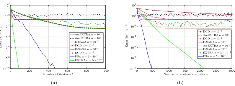
Fig. 2 illustrates the convergence paths of DSA, EXTRA, DGD, Stochastic EXTRA, and Decen-tralized SAGA with constant stepsizes forN = 20 nodes. For EXTRA and DSA different stepsizes are chosen and the best performance for EXTRA and DSA are achieved by α = 5×10⁻² and
0 200 400 600 800 1000 Number of itrationst
10-10 10-8 10-6 10-4 10-2 100 102
E
r
r
or
k
x
t−
x
∗k
2
sto-EXTRAα= 10−3
sto-EXTRAα= 10−2
D-SAGAα= 10−2
DGDα= 10−2
D-SAGAα= 10−3
DGDα= 10−3
DSAα= 5×10⁻³
EXTRAα= 5×10⁻²
(a)
0 500 1000 1500 2000 2500 3000
Number of gradient evaluations 10-10
10-8 10-6 10-4 10-2 100 102
E
rr
or
k
x
t−
x
∗k
2
DGDα= 10−3 sto-EXTRAα= 10−2 DGDα= 10−2 D-SAGAα= 10−2 sto-EXTRAα= 10−3 D-SAGAα= 10−3 EXTRAα= 5×10⁻² DSAα= 5×10⁻³
(b)
Figure 2: Convergence paths of DSA, EXTRA, DGD, Stochastic EXTRA, and Decentralized SAGA for a logistic regression problem with Q= 500 samples andN = 20 nodes. Distance to optimalityet=kxt−x∗k2 is shown with respect to number of iterationstand number of
gradient evaluations in Fig 2(a) and Fig. 2(b), respectively. DSA and EXTRA converge linearly to the optimal argument x∗, while DGD, Stochastic EXTRA, and Decentralized SAGA with constant step sizes converge to a neighborhood of the optimal solution. Smaller choice of stepsize for DGD, Stochastic EXTRA, and Decentralized SAGA leads to a more accurate convergence, while the speed of convergence becomes slower. DSA outperforms EXTRA in terms of number of gradient evaluations to achieve a target accuracy.
order O(µ/L2). As shown in Fig. 2, DSA is the only stochastic algorithm that converges linearly. Decentralized SAGA after a few iterations achieves the performance of DGD and they both cannot converge to the optimal argument. By choosing a smaller stepsize asα= 10−3, they reach a more accurate convergence relative to the case that the stepsize is α= 10−2; however, the speed of
con-vergence is slower for the smaller stepsize. Stochastic EXTRA also suffers from inexact concon-vergence, but for a different reason. DGD and decentralized SAGA have inexact convergence since they solve a penalty version of the original problem, while stochastic EXTRA can not reach the optimal solution since the noise of stochastic gradient is not vanishing. DSA resolves both issues by combining the idea of stochastic averaging from SAGA to control the noise of stochastic gradient estimation and the double descent idea of EXTRA to solve the correct optimization problem.
Fig. 2(a) illustrates convergence paths of the considered methods in terms of number of iterations
t. Notice that the number of iterations t indicates the number of local iterations processed at each node. Convergence rate of EXTRA is faster than DSA in terms of number of iterations or equivalently number of communications as shown in Fig. 2(a); however, the complexity of each iteration for EXTRA is higher than DSA. Therefore, it is reasonable to compare the performances of these algorithms in terms of number of processed feature vectors or equivalently number of gradient evaluations. For instance, DSA requires t= 380 iterations or equivalently 380 gradient evaluations to achieve the erroret= 10−8, while to achieve the same accuracy EXTRA requirest= 69 iterations
0 500 1000 1500 2000
Number of iterationst
10-8
10-6
10-4
10-2
100
102
E
rr
or
k
x
t−
x
∗k
2
Line Cycle
Random graphpc= 0.25
Random graphpc= 0.35
Complete graph
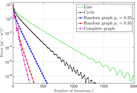
Figure 3: Convergence of DSA for different network topologies when the total number of samples is Q= 500 and the size of network is N = 50. Distance to optimalityet=kxt−x∗k2 is shown with respect to number of iterationst. As the graph condition numberκg becomes larger the linear convergence of DSA becomes slower. The best performance belongs to the complete graph which has the smallest condition number and the slowest convergence path belongs to the line graph which has the largest graph condition number.
per iteration, while in the deterministic methods each node requires q gradient evaluations per iteration. The convergence paths in Fig. 2(b) showcase the advantage of DSA relative to EXTRA in requiring less processed feature vectors (or equivalently gradient evaluations) for achieving a specific accuracy. It is important to mention that the initial gradient evaluations for the DSA method is not considered in Fig. 2(b) since the initial decision variable isx0=0in all experiments and evaluation of the initial gradients∇fn,i(x0) =−(1/2)qln,isn,i is not computationally expensive relative to the general gradient computation which is given by∇fn,i(x) = (λx/N)−(qln,isn,i)/(1 + exp(ln,ixTsn,i)). However, if we consider this initial processing the plot for DSA in Fig. 2(b) will be shifted byq= 25 gradient evaluations which doesn’t change the conclusion that DSA outperforms EXTRA in terms of gradient evaluations
4.2 Effect of Graph Condition Number κg
In this section we study the effect of the graph condition number κg as defined in (44) on the performance of DSA. We keep the parameters in Fig. 2 except for the network size N which we set as N = 50. Thus, each node has access toq = 500/50 = 10 sample points. The convergence paths of the DSA algorithm for random networks with pc = 0.25 and pc = 0.35, complete graph, cycle, and line are shown in Fig. 3. Notice that the graph condition number of the line graph, cycle graph, random graph withpc = 0.25, random graph withpc = 0.35, and complete graph are
κg= 1.01×10³,κg= 2.53×10²,κg= 17.05,κg= 4.87, andκg= 4, respectively. For each network topology, we have hand-optimized the stepsize α and the best choice of stepsize for the complete graph, random graph withpc= 0.35, random graph withpc= 0.25, cycle, and line areα= 2×10⁻²,
α= 1.5×10⁻²,α= 10−2,α= 5×10⁻³, andα= 3×10⁻³, respectively.
As we expect for the topologies that the graph has more edges and the graph condition number
0 200 400 600 800 1000 Number of gradient evaluations
10-10 10-8 10-6 10-4 10-2 100 102
E
rr
or
k
x
t−
x
∗k
2
EXTRA for complete graph DSA for complete graph
(a) complete graph
0 200 400 600 800 1000 1200
Number of gradient evaluations
10-10 10-8 10-6 10-4 10-2 100 102
E
rr
or
k
x
t−
x
∗k
2
EXTRA for random graph withpc= 0.35
DSA for random graph withpc= 0.35
(b) random graphpc= 0.35
0 500 1000 1500 2000
Number of gradient evaluations
10-10
10-8
10-6
10-4
10-2
100
102
E
rr
or
k
x
t−
x
∗k
2
EXTRA for random graph withpc= 0.25 DSA for random graph withpc= 0.25
(c) random graphpc= 0.25
0 2000 4000 6000 8000 10000 12000 14000 16000
Number of gradient evaluations
10-8 10-6 10-4 10-2 100 102
E
rr
or
k
x
t−
x
∗k
2
EXTRA for line DSA for line
(d) line
Figure 4: Convergence paths of DSA and EXTRA for different network topologies when the total number of samples isQ= 500 and the size of network isN = 50. Distance to optimality
et=kxt−x∗k2is shown with respect to number of gradient evaluations. DSA converges
faster relative to EXTRA in all of the considered networks. The difference between the convergence paths of DSA and EXTRA is more substantial when the graph has a large condition number κg. The stepsize αfor DSA and EXTRA in all the considered cases is hand-optimized and the results for the best choice ofαare reported.
complete graph which requires t = 247 iterations to achieve the relative error et = 10−8. In the
random graphs with connectivity probabilities pc = 0.35 andpc = 0.25, DSA achieves the relative erroret= 10−8 aftert= 310 andt= 504 iterations, respectively. For the cycle and line graphs the
numbers of required iterations for reaching the relative error et= 10−8 aret= 1133 and t= 1819,
respectively. These observations match the theoretical result in (47) that DSA converges faster when the graph condition numberκg is smaller.
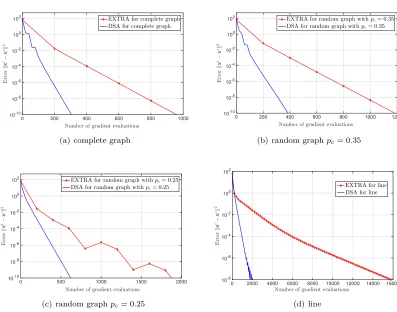
We also compare the performances of DSA and EXTRA over different topologies to verify the claim that DSA is more efficient than EXTRA in terms of number of gradient evaluations over different network topologies. The parameters are as in Fig. 3 and the stepsize α for EXTRA in different topologies are optimized separately. In particular, the best stepsize for the complete graph, random graph withpc= 0.35, random graph withpc= 0.25, and line areα= 6×10⁻²,α= 5×10⁻²,
0 1000 2000 3000 4000 5000
Number of iterationst
10-10 10-8 10-6 10-4 10-2 100 102
er
ror
k
x
t−
x
∗k
2
Q= 100,q= 5
Q= 500,q= 25
Q= 1000,q= 50
Q= 5000,q= 250
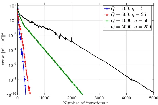
Figure 5: Comparison of convergence paths of DSA for different number of samples Q when the network size is N = 20 and the graph is randomly generated with the connectivity ratio
pc= 0.35. Convergence time for DSA increases by increasing the total number of sample pointsQwhich is equivalent to increasing the number of samples at each nodeq=Q/N.
that in the considered graphs, DSA achieves a target accuracykxt−x∗k2 faster than EXTRA. In
other words, to achieve a specific accuracykxt−x∗k2 DSA requires less number of local gradient
evaluations relative to EXTRA. In addition, the gap between the performance of DSA and EXTRA is more substantial when the graph condition number κg is larger. In particular, in the case that we have a complete graph, which has a small graph condition number, the difference between the convergence paths of DSA and EXTRA is less significant comparing to the line graph which has a large graph condition number.
4.3 Effect of Number of Functions (Samples) at Each Node q
To evaluate performance for different number of functions (sample points) available at each node which is indicated byq, we use the same setting as in Fig. 2; however, we consider scenarios with different number of samplesQwhich leads to different number of samples at each nodeq. To be more precise, we fix the total number of nodes in the network asN= 20 and we consider the cases that the total number of samples areQ= 100,Q= 500,Q= 1000, andQ= 5000 where the corresponding number of samples at each node areq= 5,q= 25,q= 50, andq= 250, respectively. Similar to the experiment in Fig. 2, the graph is generated randomly with connectivity ratiopc= 0.35.
For each of these scenarios the DSA stepsize α is hand-optimized and the best choice is used for comparison with others. The results are reported for α = 10−4, α = 10−3, α = 5×10⁻³, and α = 10−1 when the total number of samples are Q = 5000, Q = 1000, Q = 500, Q = 100, respectively. The resulting convergence paths are shown in Fig. 5.
0 100 200 300 400 500 600 700 800 900
Number of gradient evaluations
10-10
10-8
10-6
10-4
10-2
100
102
er
ror
k
x
t−
x
∗k
2
DSA EXTRA
(a) Q= 100,q= 5
0 500 1000 1500 2000 2500
Number of gradient evaluations
10-10
10-8
10-6
10-4
10-2
100
102
er
ror
k
x
t−
x
∗k
2
DSA EXTRA
(b)Q= 500,q= 25
0 1000 2000 3000 4000 5000
Number of gradient evaluations
10-10 10-8 10-6 10-4 10-2 100 102
er
ror
k
x
t−
x
∗k
2
DSA EXTRA
(c)Q= 1000,q= 50
0 1 2 3 4 5 6
Number of gradient evaluations ×104 10-10
10-8 10-6 10-4 10-2 100 102
er
ror
k
x
t−
x
∗k
2
DSA EXTRA
(d)Q= 5000,q= 250
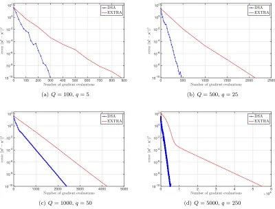
Figure 6: Convergence paths of DSA and EXTRA for the cases that (Q= 100, q= 5), (Q= 500, q= 25), (Q= 1000, q = 50), and (Q= 5000, q = 250) are presented. Distance to optimality
et=kxt−x∗k2is shown with respect to number of gradient evaluations. The total number
of nodes in the network is fixed and equal toN = 20 and the graph is randomly generated with the connectivity ratio pc= 0.35. DSA converges faster relative to EXTRA and they both converge slower when the total number of samplesQincreases.
iterations (or equivalently gradient evaluations) for the cases thatq= 5, q= 25, q= 50, q= 250, respectively.
To have a more comprehensive comparison of DSA and EXTRA, we also compare their per-formances under the four different settings considered in Fig. 5. The convergence paths of these methods in terms of number of gradient evaluations for (Q = 100, q = 5), (Q = 500, q = 25), (Q = 1000, q = 50), and (Q = 5000, q = 250) are presented in Fig 6. The optimal stepsizes for EXTRA in the considered settings areα= 4×10⁻¹,α= 5×10⁻²,α= 3×10⁻², and α=×10−2,
0 500 1000 1500
Number of iterationst
10-16
10-14
10-12
10-10
10-8
10-6
10-4
10-2
100
Nor
m
al
iz
e
d
e
r
r
or
k
x
t−
x
∗k
2
k
x
0−
x
∗k
2
DSA forN= 250
DSA forN= 125
DSA forN= 100
DSA forN= 50
DSA forN= 10
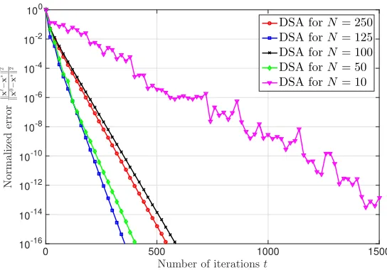
Figure 7: Normalized errorkxt−x∗k2/kx0−x∗k2of DSA versus number of iterationstfor networks
with different number of nodes N when the total number of samples is fixed Q = 500. The graphs are randomly generated with the connectivity ratiopc = 0.35. Picking a very small or large value forN which leads to a very large or small value forq, respectively, is not preferable. The best performance belongs to the case thatN = 125 andq= 4.
4.4 Effect of Number of Nodes N
In some settings, we can choose the number of nodes (processors)N for training the dataset. In this section, we study the effect of network sizeN on the convergence path of DSA when a fixed number of samplesQis given to train the classifierx. Notice that whenQis fixed, by changing the number of nodes N, the number of assigned samples to each nodeq=Q/N changes proportionally. Then, we may want to pick the number of nodesN or equivalently the number of assigned samples to each nodeqwhich leads to the best performance of DSA for trainingQsamples. Hence, we fix the total number of sample points asQ= 500 and assign the same amount of sample pointsq to each node. We consider 5 different settings withN = 10,N = 50,N = 100,N = 125, andN = 250 which their corresponding number of assigned samples to each node areq= 50,q= 10,q= 5,q= 4, andq= 2, respectively. The DSA stepsize for each of the considered settings is hand-optimized. The stepsizes
α= 5×10⁻³,α= 2×10⁻²,α= 6×10⁻², and α= 8×10⁻² are considered for the cases that the number of assigned samples to each node areq= 50,q= 10,q= 5,q= 4, andq= 2, respectively.
Fig. 7 shows the convergence paths of DSA for networks with different number of nodes. Notice that the normalized error ˜et=kxt−x∗k2/kx0−x∗k2is reported, since the dimension of the vectorx
0 500 1000 1500 2000 2500 3000 3500 4000
Number of gradient evaluations
10-15 10-10 10-5 100
Nor
m
al
iz
ed
er
ror
k
x
t−x
∗k
2
k
x
0−x
∗k
2
EXTRA forN= 10 DSA forN= 10
(a)N= 10 andq= 50
0 100 200 300 400 500 600 700 800
Number of gradient evaluations
10-15
10-10
10-5
100
Nor
m
al
iz
ed
er
ror
k
x
t−
x
∗k
2
k
x
0−x
∗k
2
EXTRA forN= 50 DSA forN= 50
(b)N= 50 andq= 10
0 200 400 600 800 1000 1200
Number of gradient evaluations
10-15
10-10
10-5
100
Nor
m
al
iz
ed
er
ror
k
x
t−x
∗k
2
k
x
0−x
∗k
2
EXTRA forN= 125
DSA forN= 125
(c)N= 125 andq= 4
0 100 200 300 400 500 600 700 800 900
Number of gradient evaluations
10-15
10-10
10-5
100
Nor
m
al
iz
ed
er
ror
k
x
t−x
∗k
2
k
x
0−
x
∗k
2
EXTRA forN= 250 DSA forN= 250
(d)N= 250 andq= 2
Figure 8: Convergence paths of DSA and EXTRA for different different number of nodesN when the total number of sample points is fixed as Q= 500. The graphs are randomly generated with the connectivity ratio pc = 0.35. Normalized distance to optimality ˜et = kxt− x∗k2/kx0−x∗k2is shown with respect to number of gradient evaluations. DSA converges
faster relative to EXTRA in all of the considered settings.
We also study the convergence rates of DSA and EXTRA in terms of number of gradient evalu-ations for networks with different number of nodesN. Fig. 8 demonstrates the convergence paths of DSA and EXTRA for the cases that N = 10, N = 50, N = 125, and N = 250. Similar to DSA, we report the best performance of EXTRA for each setting which is achieved by the stepsizes
α = 5×10⁻², α= 8×10⁻², α = 8×10⁻², and α = 10−1 for N = 10, N = 50, N = 125, and
N = 250, respectively. Observe that in all settings DSA is more efficient relative to EXTRA and it requires less number of gradient evaluations for convergence.
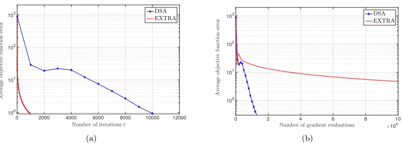
4.5 Large-scale Classification Application
In this section we solve the logistic regression problem in (48) for the protein homology dataset provided in KDD Cup 2004. The dataset contains Q= 1.45×10⁵ sample points and each sample
point hasp= 74 features. We consider the case that the sample points are distributed overN = 200 nodes which implies that each node has access toq = 725 samples. We set the connectivity ratio
pc= 0.35 and hand optimize the stepsizeαfor DSA and EXTRA separately. The best performance of DSA is observed forα= 2×10⁻⁷ and the best choice of stepize for EXTRA is α= 6×10⁻⁷. We capture the error in terms of the average objective function error et