Adaptive Lasso and group-Lasso for functional Poisson
regression
St´ephane Ivanoff [email protected]
CEREMADE UMR CNRS 7534 Universit´e Paris Dauphine F-75775 Paris, France
Franck Picard [email protected]
Laboratoire de Biom´etrie et Biologie ´Evolutive, UMR CNRS 5558 Univ. Lyon 1
F-69622 Villeurbanne, France
Vincent Rivoirard [email protected]
CEREMADE UMR CNRS 7534 Universit´e Paris Dauphine F-75775 Paris, France
Editor: Zhihua Zhang
Abstract
High dimensional Poisson regression has become a standard framework for the analysis of massive counts datasets. In this work we estimate the intensity function of the Poisson regression model by using a dictionary approach, which generalizes the classical basis ap-proach, combined with a Lasso or a group-Lasso procedure. Selection depends on penalty weights that need to be calibrated. Standard methodologies developed in the Gaussian framework can not be directly applied to Poisson models due to heteroscedasticity. Here we provide data-driven weights for the Lasso and the group-Lasso derived from concen-tration inequalities adapted to the Poisson case. We show that the associated Lasso and group-Lasso procedures satisfy fast and slow oracle inequalities. Simulations are used to assess the empirical performance of our procedure, and an original application to the analysis of Next Generation Sequencing data is provided.
Keywords: Functional Poisson regression, adaptive lasso, adaptive group-lasso, calibra-tion, concentration
Introduction
Poisson functional regression has become a standard framework for image or spectra anal-ysis, in which case observations are made ofnindependent couples (Yi, Xi)i=1,...,n, and can
be modeled as
TheXi’s (random or fixed) are supposed to lie in a known compact support ofRd(d≥1), say [0,1]d, and the purpose is to estimate the unknown intensity function f0 assumed to be positive. Wavelets have been used extensively for intensity estimation, and the statistical challenge has been to propose thresholding procedures in the spirit of Donoho and Johnstone (1994), that were adapted to the variance’s spatial variability associated with the Poisson framework. An early method to deal with high dimensional count data has been to apply a variance stabilizing-transform (see Anscombe (1948)) and to treat the transformed data as if they were Gaussian. More recently, the same idea has been applied to the data’s decomposition in the Haar-wavelet basis, see Fryzlewicz and Nason (2004) and Fryzlewicz (2008), but these methods rely on asymptotic approximations and tend to show lower performance when the level of counts is low (see Besbeas et al. (2004)). Dedicated wavelet thresholding methods were developed in the Poisson setting by Kolaczyk (1999) and Sardy et al. (2004), and a recurrent challenge has been to define an appropriate threshold like the universal threshold for shrinkage and selection, as the heteroscedasticity of the model calls for component-wise thresholding.
In this work we first propose to enrich the standard wavelet approach by considering the so-called dictionary strategy. We assume that logf0 can be well approximated by a linear combination ofpknown functions, and we reduce the estimation off0 to the estima-tion ofp coefficients. Dictionaries can be built from classical orthonormal systems such as wavelets, histograms or the Fourier basis, which results in a framework that encompasses wavelet methods. Considering overcomplete (ie redundant) dictionaries is efficient to cap-ture different feacap-tures in the signal, by using sparse representations (see Chen et al. (2001) or Tropp (2004)). For example, if logf0 shows piece-wise constant trends along with some periodicity, combining both Haar and Fourier bases will be more powerful than separate strategies, and the model will be sparse in the coefficients domain. To ensure sparse es-timations, we consider the Lasso and the group-Lasso procedures. Group estimators are particularly well adapted to the dictionary framework, especially if we consider dictionar-ies based on a wavelet system, for which it is well known that coefficients can be grouped scale-wise for instance (see Chicken and Cai (2005)). Finally, even if we do not make any assumption on p itself, it may be larger than n and methodologies based on `1-penalties, such as the Lasso and the group-Lasso appear appropriate.
consid-ered in survival analysis. See for instance Ga¨ıffas and Guilloux (2012), Zou (2008), Kong and Nan (2014), Bradic et al. (2011), Lemler (2013) and Hansen et al. (2014).
Here we consider not only the Lasso estimator but also its extension, the group-Lasso proposed by Yuan and Lin (2006), which is relevant when the set of parameters can be par-titioned into groups. The analysis of the group-Lasso has been led in different contexts. For instance, consistency has been studied by Bach (2008), Obozinski et al. (2011) and Wei and Huang (2010). In the linear model, Nardi and Rinaldo (2008) derived conditions ensuring various asymptotic properties such as consistency, oracle properties or persistence. Still for the linear model, Lounici et al. (2011) established oracle inequalities and, in the Gaussian setting, pointed out advantages of the group-Lasso with respect to the Lasso, generalizing the results of Chesneau and Hebiri (2008) and Huang and Zhang (2010). We also mention Meier et al. (2008) who studied the group-Lasso for logistic regression, Blazere et al. (2014) for generalized linear model with Poisson regression as a special case and Dalalyan et al. (2013) for other linear heteroscedastic models.
As pointed out by empirical comparative studies (see Besbeas et al. (2004)), the cal-ibration of any thresholding rule is of central importance. Here we consider Lasso and group-Lasso penalties of the form
pen(β) =
p X
j=1 λj|βj|
and
peng(β) =
K X
k=1
λgkkβGkk2,
whereG1∪ · · · ∪GK is a partition of{1, . . . , p}into non-overlapping groups (see Section 1
for more details). By calibration we refer to the definition and to the suitable choice of the weights λj and λgk, which is intricate in heteroscedastic models, especially for the
group-Lasso. For functional Poissonian regression, the ideal shape of these weights is unknown, even if for the group-Lasso, the λgk’s should of course depend on the groups size. As for the Lasso, most proposed weights in the literature are non-random and constant such that the penalty is proportional to kβk1, but when facing variable selection and consistency simultaneously, Zou (2006) showed the interest in considering non-constant data-driven `1-weights even in the simple case where the noise is Gaussian with constant variance. This issue becomes even more critical in Poisson functional regression in which variance shows spatial heterogeneity. As Zou (2006), our first contribution is to propose here adaptive procedures with weights depending on the data. Weights λj for the Lasso are derived by
on the data (see Theorem 1). We propose a similar procedure for the calibration of the group-Lasso. In most proposed procedures, the analogs of theλgk’s are proportional to the
p
|Gk|’s (see Nardi and Rinaldo (2008), B¨uhlmann and van de Geer (2011) or Blazere et al.
(2014)). But to the best of our knowledge, adaptive group-Lasso procedures (with weights depending on the data) have not been proposed yet. This is the purpose of Theorem 2, which is the main result of this work, generalizing Theorem 1 by using sharp concentration inequalities for infinitely divisible vectors. We show the shape relevance of the data-driven weights λgk by comparing them to the weights proposed by Lounici et al. (2011) in the Gaussian framework. In Theorem 2, we do not impose any condition on the groups size. However, whether|Gk|is smaller than logpor not highly influences the order of magnitude
of λgk.
Our second contribution consists in providing the theoretical validity of our approach by establishing slow and fast oracle inequalities under RE-type conditions in the same spirit as Bickel et al. (2009). Closeness between our estimates and f0 is measured by using the empirical Kullback-Leibler divergence. We show that classical oracle bounds are achieved. We also show the relevance of considering the group-Lasso instead of the Lasso in some situations. Our results, that are non-asymptotic, are valid under very general conditions on the design (Xi)i=1,...,nand on the dictionary. However, to shed some light on our results, we
illustrate some of them in the asymptotic setting with classical dictionaries like wavelets, histograms or Fourier bases. Our approach generalizes the classical basis approach and in particular block wavelet thresholding which is equivalent to group-Lasso in that case (see Yuan and Lin (2006)). We refer the reader to Chicken and Cai (2005) for a deep study of block wavelet thresholding in the context of density estimation whose framework shows some similarities with ours in terms of heteroscedasticity. Note that sharp estimation of variance terms proposed in this work can be viewed as an extension of coarse bounds provided by Chicken and Cai (2005). Finally, we emphasize that our procedure differs from Blazere et al. (2014)’s one in several aspects: First, in their Poisson regression setting, they do not consider a dictionary approach. Furthermore, their weights are constant and not data-driven, so are strongly different from ours. Finally, rates of Blazere et al. (2014) are established under much stronger assumptions than ours (see Section 3.1 for more details). Finally, we explore the empirical properties of our calibration procedures by using simulations. We show that our procedures are very easy to implement, and we compare their performance with variance-stabilizing transforms and cross-validation. The calibrated Lasso and group-Lasso are associated with excellent reconstruction properties, even in the case of low counts. We also propose an original application of functional Poisson regres-sion to the analysis of Next Generation Sequencing data, with the denoising of a Poisson intensity applied to the detection of replication origins in the human genome (see Picard et al. (2014)).
data-driven weights of our procedures that are extensively commented. Theoretical per-formance of our estimates are studied in Section 3 in the oracle approach. In Section 4, we investigate the empirical performance of the proposed estimators using simulated data, and an application is provided on next generation sequencing data in Section 5.
1. Penalized log-likelihood estimates for Poisson regression and dictionary approach
We consider the functional Poisson regression model, with n observed counts Yi ∈ N modeled such that:
Yi|Xi∼ Poisson(f0(Xi)), (1.1)
with the Xi’s (random or fixed) supposed to lie in a known compact support, say [0,1]d.
Since the goal here is to estimate the function f0 assumed to be positive on [0,1]d, a natural candidate is a function f of the form f = exp(g). Then, we consider the so-called dictionary approach which consists in decomposingg as a linear combination of the elements of a given finite dictionary of functions denoted by Υ ={ϕj}j∈J, withkϕjk2= 1 for all j. Consequently, we chooseg of the form:
g=X
j∈J
βjϕj,
with p = card(J) that may depend on n (as well as the elements of Υ). Without loss of generality we will assume in the following that J = {1, . . . , p}. In this framework, estimatingf0 is equivalent to estimating the vector of regression coefficientsβ= (βj)j∈J ∈
Rp. In the sequel, we write gβ =Pj∈J βjϕj, fβ = exp(gβ),for all β∈Rp. Note that we do not require the model to be true, that is we do not suppose the existence of β0 such that f0=fβ0.
The strength of the dictionary approach lies in its ability to capture different features of the function to estimate (smoothness, sparsity, periodicity,...) by sparse combinations of elements of the dictionary so that only few coefficients need to be selected, which lim-its estimation errors. Obviously, the dictionary approach encompasses the classical basis approach consisting in decomposing g on an orthonormal system. The richer the dictio-nary, the sparser the decomposition, so p can be larger than n and the model becomes high-dimensional.
We consider a likelihood-based penalized criterion to select β, the coefficients of the dictionary decomposition. We denote by A the n×p-design matrix with Aij = ϕj(Xi),
Y= (Y1, . . . , Yn)T and the log-likelihood associated with this model is
l(β) =X
j∈J
βj(ATY)j− n X
i=1
exp X
j∈J
βjAij
−
n X
i=1
log(Yi!),
which is a concave function of β. Next sections propose two different ways to penalize
1.1 The Lasso estimate
The first penalty we propose is based on the (weighted)`1-norm and we obtain a Lasso-type estimate by considering
b
βL∈argmin β∈Rp
−l(β) +
p X
j=1 λj|βj|
. (1.2)
The penalty term Pp
j=1λj|βj|depends on positive weights (λj)j∈J that vary according to the elements of the dictionary and are chosen in Section 2.1. This choice of varying weights instead of a unique λ stems from heteroscedasticity due to the Poisson regression, and a first part of our work consists in providing theoretical data-driven values for these weights, in the same spirit as Bertin et al. (2011) or Hansen et al. (2014) for instance. From the
first order optimality conditions (see B¨uhlmann and van de Geer (2011)),βb L
satisfies
ATj(Y−exp(Aβb L
)) = λj b
βL j
|βbjL|
ifβbjL6= 0,
|ATj(Y−exp(Aβb L
))| ≤ λj ifβbjL= 0,
where exp(Aβ) = (exp((Aβ)1), . . . ,exp((Aβ)n))T andAj is thej-th column of the matrix
A. Note that the larger the λj’s, the sparser the estimates. In particular βb L
belongs to the set of the vectorsβ∈Rp that satisfies for any j∈ J,
|ATj(Y−exp(Aβ))| ≤λj. (1.3)
The Lasso estimator off0 is now easily derived. Definition 1 The Lasso estimator of f0 is defined as
b
fL(x) := exp(bgL(x)) := exp
p X
j=1
b
βLjϕj(x) !
.
We also propose an alternative tofbL by considering the group-Lasso.
1.2 The group-Lasso estimate
We also consider the grouping of coefficients into non-overlapping blocks. Indeed, group estimates may be better adapted than their single counterparts when there is a natural group structure. The procedure keeps or discards all the coefficients within a block and can increase estimation accuracy by using information about coefficients of the same block. In our setting, we partition the set of indices J ={1, . . . , p} intoK non-empty groups:
For anyβ∈Rp,βGk stands for the sub-vector ofβ with elements indexed by the elements of Gk, and we define the block `1-norm on Rp by
kβk1,2 =
K X
k=1
kβGkk2.
Similarly,AGk is then×|Gk|submatrix ofAwhose columns are indexed by the elements of Gk. Then the group-Lassoβb
gL
is a solution to the following convex optimization problem:
b
βgL ∈argmin β∈Rp
n
−l(β) +
K X
k=1
λgkkβGkk2
o
,
where the λgk’s are positive weights for which we also provide a theoretical data-driven expression in Section 2.2. This group-estimator is constructed similarly to the Lasso, with the block`1-norm being used instead of the`1-norm. In particular, note that if all groups are of size one then we recover the Lasso estimator. Convex analysis states that βb
gL
is a solution of the above optimization problem if the p-dimensional vector 0 is in the subdifferential of the objective function. Therefore, βb
gL
satisfies:
ATGk(Y−exp(Aβb gL
)) =λgk βb
gL Gk
kβb gL Gkk2
ifβb gL Gk 6=0,
kATGk(Y−exp(Aβb gL
))k2 ≤λgk ifβb gL Gk =0.
This procedure naturally enhances group-sparsity as analyzed by Yuan and Lin (2006), Lounici et al. (2011) and references therein.
Obviously, βb gL
belongs to the set of the vectors β ∈ Rp that satisfy for any k ∈
{1, . . . , K},
kATGk(Y−exp(Aβ))k2≤λgk. (1.4) Now, we set
Definition 2 The group Lasso estimator of f0 is defined as
b
fgL(x) := exp(bggL(x)) := exp
p X
j=1
b
βjgLϕj(x) !
.
In the following our results are given conditionally on theXi’s, andE(resp. P) stands for the expectation (resp. the probability measure) conditionally on X1, . . . , Xn. In some
Definition 3 We say that the design (Xi)i=1,...,n is regular if either the design is
deter-ministic and theXi’s are equispaced in[0,1]or the design is random and the Xi’s are i.i.d.
with density h, with
0< inf
x∈[0,1]dh(x)≤ sup
x∈[0,1]d
h(x)<∞.
2. Weights calibration using concentration inequalities
Our first contribution is to derive theoretical data-driven values of the weights λj’s and
λgk’s, specially adapted to the Poisson model. In the classical Gaussian framework with noise varianceσ2, weights for the Lasso are chosen to be proportional toσ√logp(see Bickel et al. (2009) for instance). The Poisson setting is more involved due to heteroscedasticity and such simple tuning procedures cannot be generalized easily. Sections 2.1 and 2.2 give closed forms of parametersλj andλgk. They are based on concentration inequalities specific
to the Poisson model. In particular, λj is used to control the fluctuations of ATjY around
its mean, which enhances the key role of Vj, a variance term (the analog ofσ2) defined by
Vj = Var(ATjY) = n X
i=1
f0(Xi)ϕ2j(Xi). (2.1)
2.1 Data-driven weights for the Lasso procedure
For any j, we choose a data-driven value for λj as small as possible so that with high
probability, for any j∈ J,
|ATj(Y−E[Y])| ≤λj. (2.2)
Such a control is classical for Lasso estimates (see the references above) and is also a key point of the technical arguments of the proofs. Requiring that the weights are as small as possible is justified, from the theoretical point of view, by oracle bounds depending on the λj’s (see Corollaries 1 and 2). Furthermore, as discussed in Bertin et al. (2011), choosing
theoretical Lasso weights as small as possible is also a suitable guideline for practical purposes. Finally, note that if the model were true, i.e. if there existed a true sparse vector β0 such that f0 = fβ0, then E[Y] = exp(Aβ0) and β0 would belong to the set
defined by (1.3) with large probability. The smaller the λj’s, the smaller the set within
selection of βb L
is performed. So, with a sharp control in (2.2), we increase the probability to select β0. The following theorem provides the data-driven weights λj’s. The main
theoretical ingredient we use to choose the weights λj’s is a concentration inequality for
Theorem 1 Let j be fixed and γ > 0 be a constant. Define Vbj = Pn
i=1ϕ2j(Xi)Yi the
natural unbiased estimator of Vj and
e
Vj =Vbj+ r
2γlogpVbjmax
i ϕ
2
j(Xi) + 3γlogpmaxi ϕ
2
j(Xi).
Set
λj = q
2γlogpVej +
γlogp
3 maxi |ϕj(Xi)|, (2.3)
then
P
|ATj(Y−E[Y])| ≥λj
≤ 3
pγ. (2.4)
The first term
q
2γlogpVej inλj is the main one, and constitutes a variance term depending
on Vej that slightly overestimatesVj (see Section 7.1 for more details about the derivation
of Vej). Its dependence on an estimate of Vj was expected since we aim at controlling
fluctuations ofATjY around its mean. The second term comes from the heavy tail of the Poisson distribution, and is the price to pay, in the non-asymptotic setting, for the added complexity of the Poisson framework compared to the Gaussian framework.
To shed more lights on the form of the proposed weights from the asymptotic point of view, assume that the design is regular (see Definition 3). In this case, it is easy to see that under mild assumptions onf0,Vj is asymptotically of order n. If we further assume
that
max
i |ϕj(Xi)|=o( p
n/logp), (2.5)
then, when p is large, with high probability, Vbj (and then Vej) is also of order n (using
Remark 2 in the proofs Section 7.1), and the second term in λj is negligible with respect
to the first one. In this case, λj is of order
√
nlogp. Note that Assumption (2.5) is quite classical in heteroscedastic settings (see Bertin et al. (2011)). By taking the hyperparameter γ larger than 1, then for large values ofp, (2.2) is true for anyj ∈ J, with large probability.
2.2 Data-driven weights for the group Lasso procedure
Current group-Lasso procedures are tuned by choosing the analog of λgk proportional to
p
|Gk|(see Nardi and Rinaldo (2008), Chapter 4 of B¨uhlmann and van de Geer (2011) or
Blazere et al. (2014)). A more refined version of tuning group-Lasso is provided by Lounici et al. (2011) in the Gaussian setting (see below for a detailed discussion). To the best of our knowledge, data-driven weights (with theoretical validation) for the group-Lasso have not been proposed yet. It is the purpose of Theorem 2. Similarly to the previous section, we propose data-driven theoretical derivations for the weightsλgk’s that are chosen as small as possible, but satisfying for anyk∈ {1, . . . , K},
with high probability (see (1.4)). Choosing the smallest possible weights is also recom-mended by Lounici et al. (2011) in the Gaussian setting (see in their Section 3 the discus-sion about weights and comparisons with coarser weights of Nardi and Rinaldo (2008)). Obviously,λgkshould depend on sharp estimates of the variance parameters (Vj)j∈Gk. The following theorem is the equivalent of Theorem 1 for the group-Lasso. Relying on specific concentration inequalities established for infinitely divisible vectors by Houdr´e et al. (2008), it requires a known upper bound for f0, which can be chosen as max
i Yi in practice.
Theorem 2 Letk∈ {1, . . . , K}be fixed andγ >0be a constant. Assume that there exists M >0 such that for any x, |f0(x)| ≤M. Let
ck= sup
x∈Rn
kAGkA
T Gkxk2
kAT Gkxk2
. (2.7)
For all j∈Gk, still with Vbj = Pn
i=1ϕ2j(Xi)Yi,define e
Vjg=Vbj+ r
2(γlogp+ log|Gk|)Vbjmax
i ϕ
2
j(Xi) + 3(γlogp+ log|Gk|) max
i ϕ
2
j(Xi). (2.8)
Let γ >0 be fixed. Define bik=qP j∈Gkϕ
2
j(Xi) andbk = max i b
i
k. Finally, we set
λgk=
1 + 1 2√2γlogp
s X
j∈Gk
e
Vjg+ 2pγlogp Dk, (2.9)
where Dk= 8M c2k+ 16b2kγlogp. Then,
P kATGk(Y−E[Y])k2 ≥λ
g k
!
≤ 2
pγ. (2.10)
Similarly to the weights λj’s of the Lasso, each weight λgk is the sum of two terms. The
term Vejg is an estimate of Vj so it plays the same role as Vej. In particular,Vejg and Vej are
of the same order since log|Gk|is not larger than logp. The first term inλgk is a variance
term, and the leading constant 1 + 1/(2√2γlogp) is close to 1 whenpis large. So, the first term is close to the square root of the sum of sharp estimates of the (Vj)j∈Gk, as expected for a grouping strategy (see Chicken and Cai (2005)).
The second term, namely 2√γlogp Dk, is more involved. To shed light on it, sincebk
and ck play a key role, we first state the following proposition controlling values of these
terms.
Proposition 1 Let k be fixed. We have
bk≤ck≤
√
Furthermore,
c2k≤max
j∈Gk
X
j0∈G
k
n X
l=1
ϕj(Xl)ϕj0(Xl)
. (2.12)
The first inequality of Proposition 1 shows that 2√γlogp Dkis smaller thanck
√
logp+ bklogp ≤ 2cklogp up to a constant depending on γ and M. At first glance, the second
inequality of Proposition 1 shows that ck is controlled by the coherence of the dictionary
(see Tropp (2004)) and bk depends on (maxi|ϕj(Xi)|)j∈Gk. In particular, if for a given block Gk, the functions (ϕj)j∈Gk are orthonormal, then for fixed j 6= j
0, if the X
i’s are
deterministic and equispaced on [0,1] or if the Xi’s are i.i.d. with a uniform density on
[0,1]d, then, when nis large
1 n
n X
l=1
ϕj(Xl)ϕj0(Xl)≈
Z
ϕj(x)ϕj0(x)dx= 0
and we expect
c2k.max
j∈Gk
n X
l=1
ϕ2j(Xl).
In any case, by using the Cauchy-Schwarz Inequality, Condition (2.12) gives
c2k≤max
j∈Gk
X
j0∈G
k
n X
l=1
ϕ2j(Xl)
!1/2 n X
l=1
ϕ2j0(Xl)
!1/2
. (2.13)
To further discuss orders of magnitude for theck’s, we consider the following condition
max
j∈Gk
n X
l=1
ϕ2j(Xl) =O(n), (2.14)
which is satisfied for instance for fixed k if the design is regular, sincekϕjk2 = 1. Under Assumption (2.14), Inequality (2.13) gives
c2k =O(|Gk|n).
We can say more on bk and ck (and then on the order of magnitude of λgk) by considering
classical dictionaries of the literature to build the blocksGk, which is of course realized in
practice. In the subsequent discussions, the balance between|Gk|and logpplays a key role.
2.2.1 Order of magnitude of λgk by considering classical dictionaries.
Let Gk be a given block and assume that it is built by using only one of the subsequent
systems. For each example, we discuss the order of magnitude of the term Dk = 8M c2k+
16b2kγlogp. For ease of exposition, we assume thatf0 is supported by [0,1] but we could easily generalize the following discussion to the multidimensional setting.
Bounded dictionary. Similarly to Blazere et al. (2014), we assume that there exists a constantL not depending onn andp such that for anyj ∈Gk,kϕjk∞≤L.For instance,
atoms of the Fourier basis satisfy this property. We then have
b2k≤L2|Gk|.
Finally, under Assumption (2.14),
Dk=O(|Gk|n+|Gk|logp). (2.15)
Compactly supported wavelets. Consider the one-dimensional Haar dictionary: For j= (j1, k1)∈Z2 we setϕj(x) = 2j1/2ψ(2j1x−k1), ψ(x) = 1[0,0.5](x)−1]0.5,1](x).Assume that the blockGkdepends on only one resolution levelj1: Gk ={j= (j1, k1) : k1 ∈Bj1},
whereBj1 is a subset of{0,1, . . . ,2
j1−1}. In this case, since for j, j0∈G
kwithj6=j0, for
any x,ϕj(x)ϕj0(x) = 0,
b2k= max
i X
j∈Gk
ϕ2j(Xi) = max i,j∈Gk
ϕ2j(Xi) = 2j1
and Inequality (2.12) gives
c2k≤max
j∈Gk
n X
l=1
ϕ2j(Xl).
If, similarly to Condition (2.5), we assume that maxi,j∈Gk|ϕj(Xi)|=o(
p
n/logp),then
b2k =o(n/logp), and under Assumption (2.14),
Dk=O(n),
which improves (2.15). This property can be easily extended to general compactly sup-ported waveletsψ, since, in this case, for any j= (j1, k1)
Sj =
j0 = (j1, k01) : k10 ∈Z, ϕj ×ϕj0 6≡0
Regular histograms. Consider a regular grid of the interval [0,1], {0, δ,2δ, . . .} with δ > 0. Consider then (ϕj)j∈Gk such that for any j ∈ Gk, there exists ` such that ϕj = δ−1/21(δ(`−1),δ`]. We have kϕjk2 = 1 and kϕjk∞ = δ−1/2. As for the wavelet case, for
j, j0 ∈Gk withj 6=j0, for anyx,ϕj(x)ϕj0(x) = 0, then
b2k= max
i X
j∈Gk
ϕ2j(Xi) = max i,j∈Gk
ϕ2j(Xi) =δ−1.
If, similarly to Condition (2.5), we assume that maxi,j∈Gk|ϕj(Xi)|=o(
p
n/logp),then
b2k=o(n/logp), and under Assumption (2.14),
Dk =O(n).
The previous discussion shows that we can exhibit dictionaries such that c2k and Dk
are of order n and the term b2klogp is negligible with respect to c2k. Then, if similarly to Section 2.1, the terms (Vejg)j∈G
k are all of ordern,λ
g
kis of order p
n×max(logp;|Gk|) and
the main term in λgk is the first one as soon as |Gk| ≥ logp. In this case, λgk is of order p
|Gk|n.
2.2.2 Comparison with the Gaussian framework.
Now, let us compare the λgk’s to the weights proposed by Lounici et al. (2011) in the Gaussian framework. Adapting their notations to ours, Lounici et al. (2011) estimate the vectorβ0 in the modelY∼ N(Aβ0, σ2In) by using the group-Lasso estimate with weights
equal to
e
λgk= 2
r
σ2T r(AT
GkAGk) + 2|||A
T
GkAGk|||(2γlogp+
p
|Gk|γlogp)
,
where|||ATG
kAGk|||denotes the maximal eigenvalue ofA
T
GkAGk (see (3.1) in Lounici et al. (2011)). So, if |Gk| ≤logp, the above expression is of the same order as
q
σ2T r(AT
GkAGk) +
q
σ2|||AT
GkAGk|||γlogp. (2.16)
Neglecting the term 16b2kγlogpin the definition ofDk (see the discussion in Section 2.2.1),
we observe that λgk is of the same order as
s X
j∈Gk
e
Vjg+
q
M c2
kγlogp. (2.17)
Since M is an upper bound of Var(Yi) = f0(Xi) for any i, strong similarities can be
- For the first terms,Vejg is an estimate of Vj and
X
j∈Gk
Vj ≤M X
j∈Gk
n X
i=1
ϕ2j(Xi) =M×T r(ATGkAGk).
- For the second terms, in view of (2.7),c2k is related to|||ATG
kAGk|||since we have
c2k= sup x∈Rn
kAGkA
T Gkxk
2 2
kATG kxk
2 2
≤ sup
y∈R|Gk|
kAGkyk 2 2
kyk2 2
=|||ATGkAGk|||.
These strong similarities between the Gaussian and the Poissonian settings strongly support the shape relevance of the weights we propose.
2.2.3 Suboptimality of the naive procedure
Finally, we show that the naive procedure that considers qP j∈Gkλ
2
j instead of λ g k is
suboptimal even if, obviously due to Theorem 1, with high probability,
kATG
k(Y−E[Y])k2≤
s X
j∈Gk λ2
j.
Suboptimality is justified by following heuristic arguments. Assume that for alljandk, the first terms in (2.3) and (2.9) are the main ones andVej ≈Ve
g
j ≈Vj. Then by considering λgk
instead ofqP j∈Gkλ
2
j, we improve our weights by the factor
√
logp, since in this situation,
λgk ≈
s X
j∈Gk Vj
and
s X
j∈Gk λ2
j ≈ s
logp X
j∈Gk Vj ≈
p
logp λgk.
Remember that our previous discussion shows the importance to consider weights as small as possible as soon as (2.6) is satisfied with high probability. The next section will confirm this point.
3. Oracle inequalities
In this section, we establish oracle inequalities to study theoretical properties of our estima-tion procedures. TheXi’s are still assumption-free, and the performance of our procedures
we use the empirical Kullback-Leibler divergence associated with our model, denoted by K(·,·). Straightforward computations (see for instance Leblanc and Letu´e (2006)) show that for any positive functionf,
K(f0, f) = E
log
L
(f0)
L(f)
=
n X
i=1
[(f0(Xi) logf0(Xi)−f0(Xi))]−[(f0(Xi) logf(Xi)−f(Xi))],
where L(f) is the likelihood associated with f. We speak about empirical divergence to emphasize its dependence on the Xi’s. Note that we can write
K(f0, f) =
n X
i=1
f0(Xi)(eui−ui−1), (3.1)
where ui = logff0((XXi)i). This expression clearly shows that K(f0, f) is non-negative and K(f0, f) = 0 if and only if for all i∈ {1, . . . , n}, we have ui = 0, that isf(Xi) =f0(Xi)
for all i∈ {1, . . . , n}.
Remark 1 To weaken the dependence on n in the asymptotic setting, an alternative, not considered here, would consist in considering n−1K(·,·) instead of K(·,·).
If the classical L2-norm is the natural loss-function for penalized least squares criteria, the empirical Kullback-Leibler divergence is a natural alternative for penalized likelihood criteria. In next sections, oracle inequalities will be expressed by usingK(·,·).
3.1 Oracle inequalities for the group-Lasso estimate
In this section, we state oracle inequalities for the group-Lasso. These results can be viewed as generalizations of results by Lounici et al. (2011) to the case of the Poisson regression model. They will be established on the set Ωg where
Ωg = n
kATG
k(Y−E[Y])k2 ≤λ
g
k ∀k∈ {1, . . . , K} o
. (3.2)
Under assumptions of Theorem 2, we have P(Ωg)≥ 1−2pKγ ≥ 1−2p1−γ. By considering γ >1, we have thatP(Ωg) goes to 1 at a polynomial rate of convergence whenpgoes to +∞.
Even if our procedure is applied with weights defined in Section 2.2, note that subsequent oracle inequalities would hold for any weights (λgk)k=1,...,K such that the associated set Ωg
has high probability. For any β∈Rp, we denote by
fβ(x) = exp
p X
j=1
βjϕj(x) !
the candidate associated withβ to estimate f0. We first give a slow oracle inequality(see for instance Bunea et al. (2007a), Ga¨ıffas and Guilloux (2012) or Lounici et al. (2011)) that does not require any assumption.
Theorem 3 OnΩg,
K(f0,fbgL)≤ inf
β∈Rp
n
K(f0, fβ) + 2 K X
k=1
λgkkβGkk2
o
. (3.3)
Note that
K X
k=1
λgkkβGkk2 ≤ max
k∈{1,...,K}λ
g
k× kβk1,2
and (3.3) is then similar to Inequality (3.9) of Lounici et al. (2011). We can improve the rate of (3.3) at the price of stronger assumptions on the matrix A. We consider the following assumptions:
Assumption 1. We assume that
m:= max
i∈{1,...,n}|logf0(Xi)|<∞.
This assumption is equivalent to assuming that f0 is bounded from below and from above by positive constants. We do not assume that m is known in the sequel.
Assumption 2. For some integer s ∈ {1, . . . , K} and some constant r, the following condition holds:
0< κn(s, r) := min (
(βTGβ)1/2
kβJk2 : |J| ≤s, β∈R
p\ {0}, X k∈Jc
λgkkβGkk2 ≤r
X
k∈J
λgkkβGkk2
)
,
where G is the Gram matrix defined by G = ATCA, where C is the diagonal matrix with Ci,i =f0(Xi). With a slight abuse, βJ stands for the sub-vector of β with elements
indexed by the indices of the groups (Gk)k∈J.
This assumption is the natural extension of the classicalRestricted Eigenvalue condition introduced by Bickel et al. (2009) to study the Lasso estimate where the`1-norm is replaced with the weighted k · k1,2-norm. In the Gaussian setting, Lounici et al. (2011) considered similar conditions to establish oracle inequalities for their group-Lasso procedure (see their Assumption (3.1)). RE-type assumptions are among the mildest ones to establish oracle inequalities (see van de Geer and B¨uhlmann (2009)). In particular, if the Gram matrix G has a positive minimal eigenvalue, saydG,min, then Assumption 2 is satisfied withκ2n(s, r)≥
the ratio maxkλ g k
minkλgk (see Appendix B.3. of Lounici et al. (2011)). Furthermore, if c0 is a
positive lower bound for f0, then for allβ∈Rp, βTGβ= (Aβ)TC(Aβ)≥c0kAβk22=c0
n X
i=1
Xp
j=1
βjϕj(Xi) 2
=c0
n X
i=1
gβ2(Xi),
withgβ =Pp
j=1βjϕj.If (ϕj)j∈J is orthonormal on [0,1]dand if the design is regular, then the last term is the same order as
n
Z
g2β(x)dx=nkβk22 ≥nkβJk22
for any subsetJ ⊂ {1, . . . , K}. Under these assumptions, κ−n2(s, r) =O(n−1). We now introduce for anyµ >0
Γ(µ) =
β∈Rp : max
i∈{1,...,n}
p X j=1
βjϕj(Xi) ≤µ .
In the sequel, we restrict our attention to estimates belonging to the convex set Γ(µ). Of course, ifmwere known we would takeµ=m(orµa bit larger thanm). Note that we do not impose any upper bound onµso this condition is quite mild. The role of Γ(µ) consists in connecting K(., .) to some empirical quadratic loss functions (see the proof of Theorem 4). Alternative stronger assumptions have been considered by Lemler (2013) relying on van de Geer (2008) and Kong and Nan (2014). The value ofµonly influences constants in subsequent oracle inequalities.
We consider the slightly modified group-Lasso estimate. Letα >1 and let us set
b
βgLµ,α∈argmin β∈Γ(µ)
n
−l(β) +α
K X
k=1
λgkkβGkk2
o
, fbµ,αgL(x) = exp p X
j=1 (βb
gL
µ,α)jϕj(x) !
for which we obtain the following fast oracle inequality.
Theorem 4 Let ε >0 and s a positive integer. Let Assumption 2 be satisfied withs and
r= α+ 1 + 2α/ε α−1 .
Then, under Assumption 1, there exists a constant B(ε, m, µ) depending on ε, m and µ such that, on Ωg,
K(f0,fbµ,αgL)≤(1 +ε) inf
β∈Γ(µ)
|J(β)|≤s
(
K(f0, fβ) +B(ε, m, µ)
α2|J(β)|
κ2
n
×
max
k∈{1,...,K}λ
g k
2)
, (3.4)
The estimateβb gL
µ,α studied in Theorem 4 slightly differs from the estimate βb gL
introduced in Section 1.2 since it depends on α and minimization is only performed on Γ(µ). Both estimates coincide when µ = +∞ and when α = 1. An examination of the proof of Theorem 4 shows that limµ→+∞B(ε, m, µ) = +∞. In practice, we observe that most of
the time, with α= 1 and µlarge enough,βb gL
µ,α and βb gL
coincide. So, whenα is close to 1 and µ is large, Theorem 4 gives a good flavor of theoretical performances satisfied by our group-Lasso procedure.
Let us comment each term of the right-hand side of (3.4). The first term is an approxi-mation term, which can vanish iff0can be decomposed on the dictionary. The second term is a variance term, according to the usual terminology, which is proportional to the size of J(β). Its shape is classical in the high dimensional setting. See for instance Theorem 3.2 of Lounici et al. (2011) for the group-Lasso in linear models, or Theorem 6.1 of Bickel et al. (2009) and Theorem 3 of Bertin et al. (2011) for the Lasso. If the order of magnitude ofλgk is pn×max(logp;|Gk|) (see Section 2.2.1) and if κ−n2 =O(n−1), the order of magnitude
of this variance term is not larger than |J(β)| ×max(logp;|Gk|). Finally, if f0 can be well
approximated (for the empirical Kullback-Leibler divergence) by a group-sparse combina-tion of the funccombina-tions of the diccombina-tionary, then the right hand side of (3.4) will take small values. So, the previous result justifies our group-Lasso procedure from the theoretical point of view. Note that (3.3) and (3.4) also show the interest of considering weights as small as possible.
Blazere et al. (2014) established rates of convergence under stronger assumptions, namely all coordinates of the analog ofA are bounded by a quantityL, whereL is viewed as a constant. Rates depend onL in an exponential manner and would highly deteriorate ifLdepended onnand p. So, this assumption is not reasonable if we consider dictionaries such as wavelets or histograms (see Section 2.2.1).
3.2 Oracle inequalities for the Lasso estimate
For the sake of completeness, we provide oracle inequalities for the Lasso. Theorems 3 and 4 that deal with the group-Lasso estimate can be adapted to the non-grouping strategy when we take groups of size 1. Subsequent results are similar to those established by Lemler (2013) who studied the Lasso estimate for the high-dimensional Aalen multiplicative intensity model. The block `1-norm k · k1,2 becomes the usual `1-norm and the group support J(β) is simply the support ofβ. As previously, we only work on the probability set Ω defined by
Ω =n|ATj(Y−E[Y])| ≤λj ∀j∈ {1, . . . , p} o
. (3.5)
Theorem 1 asserts that P(Ω)≥ 1−pγ3−1 that goes to 1 as soon as γ >1. As previously,
asso-ciated probability set Ω has high probability. We obtain a slow oracle inequality for fbL:
Corollary 1 On Ω,
K(f0,fbL)≤ inf
β∈Rp
n
K(f0, fβ) + 2
p X
j=1 λj|βj|
o
.
Now, let us consider fast oracle inequalities. In this framework, Assumption 2 is replaced with the following:
Assumption 3. For some integer s ∈ {1, . . . , p} and some constant r, the following condition holds:
0< κn(s, r) := min
(βTGβ)1/2
kβJk2
: |J| ≤s, β∈Rp\ {0},
X
j∈Jc
λj|βj| ≤r X
j∈J
λj|βj|
,
whereGis the Gram matrix defined byG=ATCA, whereCis the diagonal matrix with Ci,i=f0(Xi).
As previously, we consider the slightly modified Lasso estimate. Letα >1 and let us set
b
βLµ,α ∈argmin β∈Γ(µ)
n
−l(β) +α
p X
j=1 λj|βj|
o
, fbµ,αL (x) = exp p X
j=1 (βb
L
µ,α)jϕj(x) !
for which we obtain the following fast oracle inequality.
Corollary 2 Let ε >0 and s a positive integer. Let Assumption 3 be satisfied withsand
r= α+ 1 + 2α/ε α−1 .
Then, under Assumption 1, there exists a constant B(ε, m, µ) depending on ε, m and µ such that, on Ω,
K(f0,fbµ,αL )≤(1 +ε) inf
β∈Γ(µ)
|J(β)|≤s
(
K(f0, fβ) +B(ε, m, µ)α
2|J(β)| κ2
n
( max
j∈{1,...,p}λj
2)
)
,
where κn stands for κn(s, r), and J(β) is the support of β.
4. Simulation study
Simulation settings. Even if our theoretical results do not concern model selection properties, we propose to start the simulation study by considering a simple toy example such that log(f0) =Aβ0 is generated from a true sparse vector of coefficients of sizep= 2J in the Haar basis, such that J = 10 and scales j = 1,3,4 have all non-null coefficients. More details on this function can be found in our code that is freely available 1. In this setting, log(f0) can be decomposed on the dictionary and we can assess the accuracy of selection of different methods.
We then explore the empirical performance of the Lasso and the group Lasso strategies using simulations. By performance we mean the quality of reconstruction of simulated signals as our theoretical results concern reconstruction properties. We considered different forms for intensity functions by taking the standard functions of Donoho and Johnstone (1994): blocks, bumps, doppler, heavisine, to set g0. These functions do not have an exact decomposition on any dictionary considered below. The signal to noise ratio was increased by multiplying the intensity functions by a factor α taking values in{1, . . . ,7}, α = 7 corresponding to the most favorable configuration. Observations Yi were generated
such that Yi|Xi ∼ Poisson(f0(Xi)), withf0 =αexp(g0), and (X1, . . . , Xn) was set as the
regular grid of length n = 210. Each configuration was repeated 20 times. Our method was implemented using the grpLasso Rpackage of Meier et al. (2008) to which we provide our concentration-based weights (the code is fully available 1).
The basis and the dictionary frameworks. The dictionary we consider is built on the Haar basis, on the Daubechies basis with 6 vanishing moments, and on the Fourier basis, in order to catch piece-wise constant trends, localized peaks and periodicities. Each orthonormal system has n elements, which makes p = n when systems are considered separately, and p = 2n or 3n depending on the considered dictionary. For wavelets, the dyadic structure of the decomposition allows us to group the coefficients scale-wise by forming groups of coefficients of size 2q. As for the Fourier basis, groups (also of size 2q) are formed by considering successive coefficients (while keeping their natural ordering). When grouping strategies are considered, we set all groups at the same size.
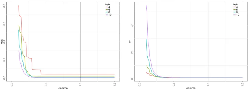
Weights calibration in practice. First for both the Lasso and the group Lasso in-troduced in Section 1, following the arguments at the end of Section 2.1 that provide some theoretical guarantees, we take γ larger than 1. More precisely, we take γ = 1.01. Our theoretical results do not provide any information about values smaller than 1, so we conduct an empirical study on a very simple case, namely we estimate f0 such that log(f0) = 1[0,1] on the Haar basis, so that only one parameter should be selected. Fig. 1 shows that whenγis too small, the risk of the selected models explodes (left panel), because too many coefficients are selected (right panel). Taking γ = 1.01 actually corresponds to a conservative choice avoiding the explosion of the MSE and of the number of selected
0.0
0.2
0.4
0.6
0.8
0.0 0.5 1.0 1.5
gamma
MSE
log2n 4 6 8 10
0
20
40
0.0 0.5 1.0 1.5
gamma
dF
log2n 4 6 8 10
Figure 1: Tuning of the hyperparameter γ for the Lasso penalty. The simulated function is log(f0) = 1[0,1], so that only one parameter should be selected on the Haar basis. For different values ofn, the left/right panels represent the mean square error / the number of estimated parameters with respect to γ (averaged over 20 simulations). The vertical line corresponds to γ = 1.
parameters. Furthermore this automatic choice provides good results in practice, as shown by our simulation study that considers many shapes of intensity functions (see below).
Then we estimate Vj (resp Vjg) by Vej (resp Vejg). Note that Vbj (resp Vbjg) can also be
used: these variances are easier to compute in practice, and this slight modification does not significantly change the performance of the procedures (not shown). The parameterγ being fixed, we use the expression (2.3) for Lasso weights. As for the group Lasso weights
(Theorem 2), the first term is replaced by
q P
j∈GkVej, as it is governed by a quantity that tends to one whenp is large. We conducted a preliminary numerical study (not shown) to calibrate the second term, that depends on quantities M, ck and bk defined in Theorem
2. The best empirical performance were achieved so that the left- and right-hand terms of (2.9) were approximatively equal. This resumes to group-Lasso weights of the form
2
q P
j∈GkVej.
by odd positions (see Nason (1996)). This procedure is referred to cross-validation in the sequel. Then we compare the performance of the group-Lasso with varying group sizes (2,4,8) to the Lasso, to assess the benefits or grouping wavelet coefficients.
Performance measurement. For any estimate ˆf, reconstruction performance were measured using the (normalized) mean-squared error M SE = kfb−f0k22/kf0k22. When
there is a true sparseβ0, model selection performance were measured by the standard in-dicators: accuracy on support recovery, sensitivity (proportion of true non-null coefficients among selected coefficients) and specificity of detection (proportion of true null coefficients among non-selected coefficients), based on the support of β0 and on the support of its estimate.
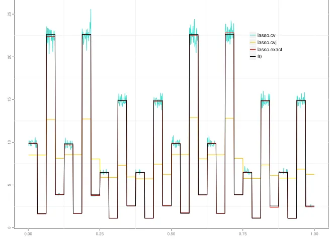
Model selection performance with a true sparse β0. The simple toy example de-scribed above for model selection perfectly shows the performance of our Lasso procedure (Figure 2). Even if our theoretical results do not concern support recovery, our theoret-ically calibrated weights provide the best accuracy in support selection, along with the best sensitivity, specificity and reconstruction errors. This example also shows the interest of the theoretical weights calibration compared with the cross-validation procedure that shows bad performance, and also compared with the Haar-Fisz transform. Also, this toy example illustrates the need of scaling for the cross-validated vanilla Lasso: if the procedure proposed by Sardy et al. (2004) is not used, the cross-validated vanilla Lasso lacks of adap-tation to heteroscedasticity, which leads to poor results on selection (lack of accuracy and specificity, or too many selected coefficients), and thus to overfitted reconstruction (Fig. 3). Thus, in further simulations we only considered the scaled version of the cross-validated Lasso, in order to compare methods that account for heteroscedasticity.
0.900
0.925
0.950
0.975
1.000
2 4 6
alpha
accur
acy
0.900
0.925
0.950
0.975
1.000
2 4 6
alpha
specificity
grplasso.2 grplasso.4 grplasso.8 HaarFisz lasso.cv lasso.cvj lasso.exact
0.00
0.25
0.50
0.75
1.00
2 4 6
alpha
sensitivity
0.2
0.4
0.6
2 4 6
alpha
mse
0
5
10
15
20
25
0.00 0.25 0.50 0.75 1.00
lasso.cv lasso.cvj lasso.exact f0
0.1
0.2
0.3
0.4
0.5
2 4 6
alpha
mse
blocks
0.225
0.250
0.275
0.300
0.325
2 4 6
alpha
mse
bumps
0.1
0.2
0.3
0.4
0.5
2 4 6
alpha
mse
doppler
0.1
0.2
0.3
0.4
2 4 6
alpha
mse
lasso.exact lasso.cvj grplasso.2
grplasso.4 grplasso.8 HaarFisz
heavi
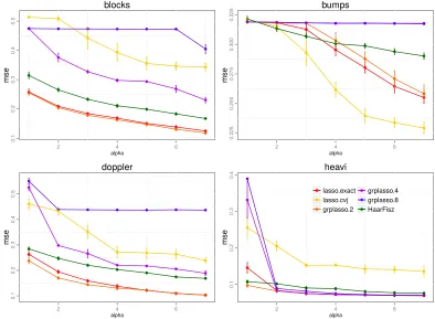
Figure 4: Average (over 20 repetitions) Mean Square Error of reconstruction of different methods for the estimation of simulated intensity functions according to function shapes (blocks, bumps, doppler, heavisine) and signal strength (α). Lasso.exact: Lasso penalty with our data-driven theoretical weights,Lasso.cvj: Lasso penalty with weights calibrated by cross validation with scaling 2s/2λ,group.Lasso.2/4/8: group Lasso penalty with our data-driven theoretical weights with group sizes 2/4/8, HaarFisz: Haar-Fisz tranform followed by soft-thresholding.
4 and 5b), since they are not scaled to the size of the irregularities in the signal. This trend is not systematic as the group Lasso appears to be adapted to functions that are more regular (Heavisine), and seems to avoid edge effects in some situations.
the best choice in terms of reconstruction error, which is stricking in the case of theblocks
function. In this case the Haar system only would be preferable for the Lasso (Figure 6a). For the group-Lasso and theblocksintensity function, the combination of the Daubechies and the Haar systems provides the best MSE, but when looking at the reconstructed intensity (Figure 6b-blocks), the Daubechies system introduces wiggles that are not relevant for blocks. Also, richer dictionaries do not necessarily lead to more selected parameters (Figure 6a), which illustrates that selection depends on the redundancies between the systems elements of the dictionary. In practice we often do not have anyprior knowledge concerning the elements that shape the signal, and these simulations suggest that the blind use of the richest dictionary may not be the best strategy in terms of reconstructed functions. Consequently, in the following application, we propose to adapt the half-fold cross validation of Nason (1996) to choose the best combinations of systems.
5. Applications
The analysis of biological data has faced a new challenge with the extensive use of next gen-eration sequencing (NGS) technologies. NGS experiments are based on the massive parallel sequencing of short sequences (reads). The mapping of these reads onto a reference genome (when available) generates counts data (Yt) spatially organized (in 1D) along the genome
(at position Xt). These technologies have revolutionized the perspectives of many fields
0
10
20
30
0.00 0.25 0.50 0.75 1.00
blocks
5
10
15
20
25
0.00 0.25 0.50 0.75 1.00
bumps
0
5
10
15
20
25
0.00 0.25 0.50 0.75 1.00
doppler
0
10
20
0.00 0.25 0.50 0.75 1.00
lasso.exact lasso.cvj HaarFisz f0 heavi
(a) Average reconstructed functions for the Lasso and competitors.
0
10
20
30
0.00 0.25 0.50 0.75 1.00
blocks
5
10
15
20
25
0.00 0.25 0.50 0.75 1.00
bumps
0
5
10
15
20
25
0.00 0.25 0.50 0.75 1.00
doppler
0
10
20
0.00 0.25 0.50 0.75 1.00
lasso.exact grplasso.2 grplasso.4 grplasso.8 f0 heavi
(b) Average reconstructed functions for the group strategies.
Figure 5: Average (over 20 repetitions) reconstructed functions by different methods of estimation according to function shapes (blocks, bumps, doppler, heavisine). Top panel corresponds to non-grouped strategies (5a) and bottom panel compares group-strategies to the Lasso (5b). Lasso.exact: Lasso penalty with our data-driven theoretical weights,
Lasso.cvj: Lasso penalty with weights calibrated by cross validation with scaling 2s/2λ,
group.Lasso.2/4/8: group Lasso penalty with our data-driven theoretical weights with group sizes 2/4/8, HaarFisz: Haar-Fisz tranform followed by soft-thresholding,f0:
D DF DFH DH F FH H H D DF DFH DH F FH H 0.15 0.16 0.17 0.18 0.19
25 35 45 55 65
df MSE a a a grplasso.2 HaarFisz lasso blocks D DF DFH DH F FH H D
DDH DFH DF
F FH H 0.26 0.27 0.28 0.29 0.30 0.31
5.0 7.5 10.0 12.5
df MSE a a a grplasso.2 HaarFisz lasso bumps D
DF DHDFH
F
FH H D
D DF DFH
DH F FH H 0.125 0.150 0.175
30 40 50
df MSE a a a grplasso.2 HaarFisz lasso doppler DDF DFH DH F FH H D D DF DFH DH F FH H 0.07 0.09 0.11 0.13
7.5 10.0 12.5 15.0
df MSE a a a grplasso.2 HaarFisz lasso heavi
(a) Average Mean Square Error for different dictionaries with respect to the average number of selected coefficients (df).
0
10
20
30
0.00 0.25 0.50 0.75 1.00
grplasso.2 + DH HaarFisz + H lasso + H truth blocks 5 10 15 20 25
0.00 0.25 0.50 0.75 1.00
grplasso.2 + DFH HaarFisz + D lasso + D truth bumps 0 5 10 15 20
0.00 0.25 0.50 0.75 1.00
grplasso.2 + DFH HaarFisz + D lasso + D truth doppler 0 5 10 15 20 25
0.00 0.25 0.50 0.75 1.00
grplasso.2 + DFH HaarFisz + D lasso + DFH truth
heavi
(b) Reconstructed functions for the dictionaries with the smallest MSE.
Figure 6: Average (over 20 repetitions) Mean Square Errors and number of selected coef-ficients (df) (6a), and reconstructed functions (6b) for different dictionaries: Daubechies (D), Fourier (F), Haar (H) and their combinations. Lasso.exact: Lasso penalty with our data-driven theoretical weights, group.Lasso.2: group Lasso penalty with our data-driven theoretical weights with group sizes 2, HaarFisz: Haar-Fisz tranform followed by
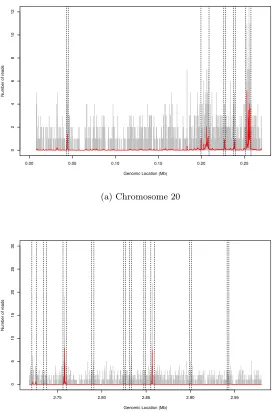
positions 0.20 and 0.25Mb, Figure 7a), which indicates that the dictionary approach may be more sensitive to detect peaks. Given the spread of NGS data and the importance of peak detection in the analysis process, for chIP-Seq Furey (2012), FAIRE-Seq Thurman et al. (2012), OriSeq Picard et al. (2014), our preliminary results suggest that the sparse dictionary approach will be a very promising framework for the analysis of such data.
6. Conclusion
We proposed new adaptive Lasso and group-Lasso procedures to estimate the regression function in high dimensional Poisson regression, with a special focus on the calibration of weights involved in the penalties. Inspired from the adaptive Lasso procedure proposed by Zou (2006) in the context of model selection, we derived data-driven component-specific weights, whose shape appears to be relevant from both theoretical and practical points of view. In the dictionary approach, which extends the classical basis approach, we obtain slow and fast oracle inequalities under RE-type conditions. These theoretical results are enhanced by a numerical study that illustrates the good performance of our procedure on simulated and experimental data. Moreover, even if our main objective is functional reconstruction (that is different from model selection), a numerical toy example shows very promising results of our Lasso and group-Lasso procedures for model selection. The theoretical study of this problem is an exciting challenge we wish to investigate in further works.
The purpose of our data-driven weights is to control the random fluctuations of the normalized observations, namely (AT
jY)j and (ATGkY)k, around their expectation. To ob-tain controls as sharp as possible, we use concentration inequalities for infinitely divisible vectors, which allows us to account for the heteroscedasticity that characterizes the Poisson setting. So, our approach is very different from Zou (2006) who considered weights propor-tional to the inverse of preliminary estimates (ordinary least squares estimates or maximum likelihood estimates). But both approaches confirm that random weighting schemes can provide suitable procedures for inference in regression models.
Finally, we mention that the constants of our procedure were tuned by using theoret-ical arguments, and our numertheoret-ical studies show that they are suitable. Other values for
0.00 0.05 0.10 0.15 0.20 0.25
0
2
4
6
8
10
12
Genomic Location (Mb)
Number of reads
(a) Chromosome 20
2.75 2.80 2.85 2.90 2.95
0
5
10
15
20
25
30
Genomic Location (Mb)
Number of reads
(b) Chromosome X
7. Proofs
7.1 Proof of Theorem 1
We denote byµthe Lebesgue measure onRdand we introduce a partition of the set [0,1]d denoted ∪n
i=1Si so that for any i= 1, . . . , n, Xi ∈ Si and µ(Si) > 0. Let h the function
defined for anyt∈[0,1]d by
h(t) =
n X
i=1
f0(Xi)
µ(Si)
1Si(t).
Finally, we introduce N the Poisson process on [0,1]d with intensity h (see Kingman (1993)). Therefore, for any i = 1, . . . , n, N(Si) is a Poisson variable with parameter R
Sih(t)dt = f0(Xi) and since ∪
n
i=1Si is a partition of [0,1]d, (N(S1), . . . , N(Sn)) has the
same distribution as (Y1, . . . , Yn). We observe that if for anyj= 1, . . . , p,
e
ϕj(t) = n X
i=1
ϕj(Xi)1Si(t),
then
Z
e
ϕj(t)dN(t)∼ n X
i=1
ϕj(Xi)Yi =ATjY.
We use the following exponential inequality (see Inequality (5.2) of Reynaud-Bouret (2003)). If gis bounded, for any u >0,
P
Z
g(x)(dN(x)−h(x)dx)≥
s
2u
Z
g2(x)h(x)dx+u 3||g||∞
!
≤exp(−u). (7.1)
By taking successivelyg=ϕej and g=−ϕej, we obtain
P |ATj(Y−E[Y])| ≥ s
2u
Z
e
ϕ2j(x)h(x)dx+u 3kϕejk∞
!
≤2e−u.
Since
Z
e
ϕ2j(x)h(x)dx=
n X
i=1
ϕ2j(Xi)f0(Xi) =Vj,
we obtain
P |ATj(Y−E[Y])| ≥ p
2uVj +
u 3kϕejk∞
!
≤2e−u. (7.2)
To controlVj, we use (7.1) with g=−ϕe
2
j and we have:
P Vj−Vbj ≥ s
2u
Z
e
ϕ4j(t)h(t)dt+ u 3kϕejk
2
∞
!
We observe that
Z
e
ϕ4j(t)h(t)dt≤ kϕejk2∞
Z
e
ϕ2j(t)h(t)dt=kϕejk2∞Vj.
Setting vj =ukϕejk
2
∞,we have:
P Vj − p
2vjVj−
vj
3 −Vbj ≥0
!
≤e−u.
Letαj = q
b
Vj+56vj+ qv
j
2,such thatαj is the positive solution toα 2
j− p
2vjαj−(Vbj+ vj
3) = 0.Then
P
Vj ≥α2j
=P
p
Vj ≥αj
≤e−u. (7.3)
We choose u =γlogp and observe that α2j ≤Vej.Then, by combining (7.2) and (7.3), we
have
P |ATj(Y−E[Y])| ≥ q
2γlogpVej +
γlogp 3 kϕejk∞
!
≤ 3
pγ.
Askϕejk∞= maxi|ϕj(Xi)|, the theorem follows.
Remark 2 By slightly extending previous computations, we easily show that for u >0,
P |Vj −Vbj| ≥ q
2uVjkϕejk
2
∞+
u 3kϕejk
2
∞
!
≤2e−u,
which leads to
P |Vj−Vbj| ≥
Vj
2 +
4γlogp 3 kϕejk
2
∞
!
≤ 2
pγ.
7.2 Proof of Theorem 2
For each k ∈ {1, . . . , K}, we recall that bik =qP j∈Gkϕ
2
j(Xi), so bik = kATGkeik2, where ei is the vector whosei-th coordinate is equal to 1 and all others to 0. We first state the
following lemma:
Lemma 1 Letkbe fixed. Assume that there exists someM >0such that∀x,|f0(x)| ≤M. Assume further that there exists someck≥0such that∀y∈Rn,kAGkA
T
Gkyk2≤ckkA
T Gkyk2. Then, ∀x >0,∀ε >0,
P kATGk(Y−E[Y])k2≥(1 +ε)
s X
j∈Gk Vj+x
!
≤exp x
bk
−x
bk
+D
ε k
b2k
log1 +bkx Dkε
!
,
Proof Withk∈ {1, . . . , K}being fixed, we definef :Rn→Rbyf(y) =
kATG
kyk2−E
+, where E > 0 is a constant chosen later. We use Corollary 1 from Houdr´e et al. (2008), applied to the infinitely divisible vectorY−E[Y]∈Rn, whose components are independent,
and to f. First note that for anyt >0,
Eetb i
k|Yi−EYi| ≤ Eetb
i
k(Yi+f0(Xi))
= expf0(Xi)(etb
i k+tbi
k−1)
<∞.
Furthermore, for any i∈ {1, ..., n}, any y∈Rn and anyu∈
R,
|f(y+uei)−f(y)| ≤ kA
T
Gk(y+uei)k2− kA
T Gkyk2
≤ kATG
k(uei)k2 = |u|bik.
Therefore, for all x >0,
P
f(Y−E[Y])−E[f(Y−E[Y])]≥x≤exp−
Z x
0
h−f1(s)ds, wherehf is defined for allt >0 by
hf(t) = sup
y∈Rn
n X
i=1
Z
R
|f(y+uei)−f(y)|2
etbik|u|−1 bi
k|u| e
νi(du)
andeνi is the L´evy measure associated withYi−E[Yi]. It is easy to show thatνei =f0(Xi)δ1,
and so
hf(t) = sup
y∈Rn
n X
i=1
f0(Xi)
f(y+ei)−f(y) 2etb
i k−1
bik .
Furthermore, writing Ai = n
kATG
k(y+ei)k2≥E orkA
T
Gkyk2≥E
o
, we have
|f(y+ei)−f(y)| ≤ kA
T
Gk(y+ei)k2− kA
T Gkyk2
1Ai
= 1Ai
kA
T
Gk(y+ei)k 2
2− kATGkyk 2 2
kATG
k(y+ei)k2+kA
T Gkyk2 =
1Ai
2<A
T Gkei,A
T
Gky>+kA
T Gkeik
2 2
kATG
k(y+ei)k2+kA
T Gkyk2
≤ 2
<A
T Gkei,A
T Gky>
kATG kyk2
+kA
T Gkeik
with <·,·>the usual scalar product. We now have
f(y+ei)−f(y) 2
≤8<A
T Gkei,A
T Gky>
2
kAT Gkyk
2 2
+ 2kA
T Gkeik
4 2 E2 . The first term can be rewritten as 8<ei,AGkA
T Gky>
2
kAT
Gkyk22
and the second one is equal to 2b i k
4
E2, so
we can now bound hf(t) as follows.
hf(t) ≤ sup
y
X
i
f0(Xi)
etbik−1 bi
k
8<ei,AGkA
T Gky>
2
kAT Gkyk
2 2
+ 2b
i k 4 E2 ! ≤ e
tbk−1
bk
sup y
8MkAGkA
T Gkyk
2 2
kAT Gkyk
2 2 + 2 E2 X i
f0(Xi)bik
4
!
≤ e
tbk−1
bk
8M c2k+ 2 E2
X
i
f0(Xi)bik
4
!
.
Now, we set
E=ε
s X
j∈Gk Vj.
So we have:
E2 = ε2 X
j∈Gk
n X
i=1
f0(Xi)ϕ2j(Xi)
= ε2
n X
i=1
f0(Xi) X
j∈Gk
ϕ2j(Xi)
= ε2
n X
i=1
f0(Xi)bik
2 .
Thus, we can finally bound the function hf by the increasing functionh defined by
h(t) =Dεke
tbk−1
bk
,
with Dkε= 8M c2k+2b
2
k
ε2 . Therefore,
exp−
Z x
0
h−f1(s)ds ≤ exp−
Z x
0
h−1(s)ds
= exp x bk
−x
bk +D ε k b2 k log
1 +bkx Dεk
!
Now,
f(Y−E[Y])−E[f(Y−E[Y])] =
kATGk(Y−E[Y])k2−E
+−E
kATGk(Y−E[Y])k2−E
+
≥ kATGk(Y−E[Y])k2−E−EkATGk(Y−E[Y])k2. Furthermore, by Jensen’s inequality, we have
EkATGk(Y−E[Y])k2 ≤
q
EkATGk(Y−E[Y])k 2 2 =
s X
j∈Gk
E[(ATj(Y−EY))2]
=
s X
j∈Gk
Var(ATjY)
=
s X
j∈Gk Vj.
Recalling that E=εqP
j∈GkVj, we thus have
P
f(Y−E[Y])−Ef(Y−E[Y])≥x≥PkATG
k(Y−E[Y])k2−(1 +ε)
s X
j∈Gk Vj ≥x
,
which concludes the proof.
We apply Lemma 1 with
ε= 1
2√2γlogp and x= 2
q
γlogpDε k.
Then,
bkx
Dεk = 2bk
√
γlogp
p
Dεk
= 2bk
√
γlogp
q
8M c2k+2b
2
k
ε2
Finally, using the fact that log(1 +u)≥u−u22, we have:
exp x bk
−x
bk
+D
ε k
b2
k
log
1 +bkx Dεk
!
≤ exp x
bk
−x
bk
+D
ε k
b2
k
bkx
Dkε − b2kx2 2Dεk2
!
= exp −x 2 2Dkε +
bkx3
2Dkε2
!
= exp −x 2 2Dkε
1− bkx
Dεk
!
≤ exp
−x2
4Dε k
= 1 pγ.
We obtain
P kATGk(Y−E[Y])k2≥(1 +ε)
s X
j∈Gk Vj+ 2
q
γlogpDεk
!
≤ 1
pγ.
We control Vj as in the proof of Theorem 1, but we takeu=γlogp+ log|Gk|. The analog
of (7.3) is
P
Vj >Ve g j
≤e−u = 1
|Gk|pγ
and thus
P
∃j∈Gk, Vj >Vejg
≤ 1
pγ.
This concludes the proof of Theorem 2.
7.3 Proof of Proposition 1
For the first point, we write:
kAGkA
T Gkxk
2 2=
n X
l=1
X
j∈Gk
ϕj(Xl) n X
i=1
ϕj(Xi)xi !2
Then, we apply the Cauchy-Schwarz inequality:
kAGkA
T Gkxk
2 2 ≤
n X
l=1
X
j∈Gk
ϕ2j(Xl) !
X
j∈Gk
Xn
i=1
ϕj(Xi)xi 2
!
= kATGkxk22
n X
l=1
X
j∈Gk
ϕ2j(Xl) !
= kATGkxk22
n X
l=1 (blk)2
≤ nb2kkATGkxk22,
which proves the upper bound of (2.11). For the lower bound, we just observe that for any i= 1, . . . , n, withei the vector whose i-th coordinate is equal to 1 and all others to 0,
bik2 = kATGkeik22
= <ATGkei,ATGkei > = <ei,AGkA
T Gkei >
≤ keik2kAGkA
T Gkeik2
≤ ckkATGkeik2 = ckbik,
which obviously entails bk≤ck. For the last point, we observe that
kATGkxk22= X