Forest response to increased disturbance in the central Amazon and comparison to western Amazonian forests

www.biogeosciences.net/11/5773/2014/ doi:10.5194/bg-11-5773-2014

© Author(s) 2014. CC Attribution 3.0 License.

Forest response to increased disturbance in the central Amazon and

comparison to western Amazonian forests

J. A. Holm1, J. Q. Chambers1,2, W. D. Collins1,3, and N. Higuchi4 1_{Lawrence Berkeley National Laboratory, Berkeley, California 94720, USA}

2_{Department of Geography, University of California, Berkeley, California 94720, USA}

3_{Department of Earth and Planetary Science, University of California, Berkeley, California 94720, USA} 4_{Departamento de Silvicultura Tropical, Manejo Florestal, Instituto Nacional de Pesquisas da Amazônia,} Av. André Araújo, 2936 Petrópolis, Manaus AM, Brasil

Correspondence to: J. A. Holm ([email protected])

Received: 10 April 2014 – Published in Biogeosciences Discuss.: 28 May 2014

Revised: 25 August 2014 – Accepted: 15 September 2014 – Published: 20 October 2014

Abstract. Uncertainties surrounding vegetation response to increased disturbance rates associated with climate change remains a major global change issue for Amazonian forests. Additionally, turnover rates computed as the average of mor-tality and recruitment rates in the western Amazon basin are doubled when compared to the central Amazon, and notable gradients currently exist in specific wood density and above-ground biomass (AGB) between these two regions. This study investigates the extent to which the variation in dis-turbance regimes contributes to these regional gradients. To address this issue, we evaluated disturbance–recovery pro-cesses in a central Amazonian forest under two scenarios of increased disturbance rates using first ZELIG-TROP, a dy-namic vegetation gap model which we calibrated using long-term inventory data, and second using the Community Land Model (CLM), a global land surface model that is part of the Community Earth System Model (CESM). Upon doubling the mortality rate in the central Amazon to mirror the natural disturbance regime in the western Amazon of∼2 % mortal-ity, the two regions continued to differ in multiple forest pro-cesses. With the inclusion of elevated natural disturbances, at steady state, AGB significantly decreased by 41.9 % with no significant difference between modeled AGB and em-pirical AGB from the western Amazon data sets (104 vs. 107 Mg C ha−1_{, respectively). However, different processes} were responsible for the reductions in AGB between the models and empirical data set. The empirical data set sug-gests that a decrease in wood density is a driver leading to the reduction in AGB. While decreased stand basal area was

the driver of AGB loss in ZELIG-TROP, a forest attribute that does not significantly vary across the Amazon Basin. Further comparisons found that stem density, specific wood density, and basal area growth rates differed between the two Amazo-nian regions. Last, to help quantify the impacts of increased disturbances on the climate and earth system, we evaluated the fidelity of tree mortality and disturbance in CLM. Similar to ZELIG-TROP, CLM predicted a net carbon loss of 49.9 %, with an insignificant effect on aboveground net primary pro-ductivity (ANPP). Decreased leaf area index (LAI) was the driver of AGB loss in CLM, another forest attribute that does not significantly vary across the Amazon Basin, and the tem-poral variability in carbon stock and fluxes was not replicated in CLM. Our results suggest that (1) the variability between regions cannot be entirely explained by the variability in dis-turbance regime, but rather potentially sensitive to intrinsic environmental factors; or (2) the models are not accurately simulating all tropical forest characteristics in response to in-creased disturbances.

1 Introduction

One of the largest uncertainties in future terrestrial sources of atmospheric carbon dioxide results from changes to forest disturbance and tree mortality rates, specifically in tropical forests (Cox et al., 2000, 2004; DeFries et al., 2002; Clark, 2007; Pan et al., 2011). There has been evidence that climate change and forest disturbance are linked such that a changing

5774 J. A. Holm et al.: Forest response to increased disturbance in the central Amazon

climate can influence the timing, duration, and intensity of disturbance regimes (Overpeck et al., 1990; Dale et al., 2001; Anderegg et al., 2013). In the tropics, climate change related impacts such as water and heat stress, and increased vulnera-bility to fires could lead to increased forest dieback (i.e., tree mortality notably higher than usual mortality) and increased disturbance rates (Cox et al., 2004; Malhi et al., 2008, 2009; US DOE, 2012). Increased forest dieback in tropical loca-tions could then produce large economic costs, ecological impacts, and lead to climate related positive feedback cycles (Canham and Marks, 1985; Dale et al., 2001; Laurance and Williamson, 2001; Bonan, 2008).

The effects of large-scale removal of tropical forest, lead-ing to changes in global climate, have been studied within global general circulation models (GCMs) (Shukla et al., 1990; Henderson-Sellers et al., 1993; Hahmann and Dick-inson, 1997; Gedney and Valdes, 2000; Avissar and Werth, 2005). For example, a rapid and complete deforestation of the diverse Amazon Basin was predicted to be irreversible (Shukla et al., 1990), losing ∼180 Gt carbon. These past studies have simulated extreme deforestation, or complete re-moval of the tropical forest biome, with the goal of evaluat-ing climate impacts (i.e., albedo, evaporation, precipitation, surface boundary conditions). However, instead of sudden and complete removal, gradual increases and spatially het-erogeneous patterns of tropical tree mortality due to multiple causes are more likely to occur than complete loss (Fearn-side 2005; Morton et al., 2006). In addition, the effective-ness of climate mitigation strategies will be affected by fu-ture changes in natural disturbances regimes (IPCC, 2014; Le Page et al., 2013), due to the effect of disturbances on the terrestrial carbon balance. By using an economic/energy integrated assessment model, it was found that when natural disturbance rates are doubled and in order to reach a stringent mitigation target, (3.7 W m−2level) the societal, technolog-ical, and economic strategies will be up to 2.5 times more costly (Le Page et al., 2013). Due to the strong feedbacks from terrestrial processes, there is a need to utilize an inte-grated Earth System Model approach (i.e., iESM; Jones et al., 2013), where an integrated assessment model is coupled with a biogeochemical and biophysical climate model such as CLM and CESM. It is necessary to improve earth system models in order to simulate dynamic disturbance rates and gradual forest biomass loss in response to increasing mortal-ity rates.

Turnover rates currently vary for different regions of Ama-zonia (Baker et al., 2004a, b; Lewis et al., 2004; Phillips et al., 2004; Chao et al., 2009), with central Amazonian forests having “slower” turnover rates, and the western and south-ern Amazonian forests (which we call “west and south”) exhibiting “faster” turnover rates. This regional variation in turnover rates is connected with differences in carbon stocks, growth rates, specific wood density, and biodiversity. Baker et al. (2004a) investigated regional-scale AGB estimates, concluding that differences in species composition and

re-lated specific wood density determined the regional patterns in AGB. There is a strong west–east gradient in that “west and south” Amazonian forests were found to have signifi-cantly lower AGB than their eastern counterparts; also con-firmed by additional studies (Malhi et al., 2006; Baraloto et al., 2011).

It is unclear if these regional variations in forest processes and carbon stocks are driven by external disturbance (e.g., in-creased drought, windstorm, forest fragmentation) or internal influences (e.g., soil quality, phosphorus limitation, species composition, wood density) (Phillips et al., 2004; Chao et al., 2009; Quesada et al., 2010; Yang et al., 2013). Inves-tigating the causes that drive variation in tree dynamics in the Amazon, in order to understand consequences for future carbon stocks for each region should still be explored. For example, are the differences in forest structure and function between the two regions a result of the disturbance regime? If the central Amazonian forests were subject to a higher distur-bance regime and turnover rates similar to that of the “west and south”, would the two regions match in terms of forest dynamics, carbon stocks and fluxes? A goal of this paper is to use modeling tools to explore the influence of disturbance regimes on net carbon stocks and fluxes in the central Ama-zon, and then compare to observational data from the “west and south” regions of the Amazon.

We are using an individual-based, demographic, gap model (Botkin et al., 1972; Shugart, 2002) as a “benchmark” model to (1) evaluate the influence of disturbance on net car-bon loss and variations in forest dynamics between two re-gions (central vs. “west and south”), (2) evaluate disturbance and mortality in CLM-CN 4.5 (called CLM for remainder of paper), and (3) improve upon representing terrestrial feed-backs more accurately in earth system modeling. We used the dynamic vegetation gap model ZELIG (Cumming and Bur-ton 1993; Urban et al., 1993). ZELIG has been updated and modified to simulate a tropical forest in Puerto Rico with a new versatile disturbance routine (ZELIG-TROP; Holm et al., 2012), making this vegetation dynamic model a good choice for this study.

independent driver of mortality; therefore, we are not assign-ing mortality to any particular cause. The final research ques-tion will evaluate the accuracy of CLM to predict changes to carbon fluxes due to increased disturbance, a process that is likely to increase with human induced climate change.

2 Methods

2.1 Study area and forest inventory plots

The empirical data used for this study were from two perma-nent transects inventoried from 1996 to 2006, located in re-serves of the National Institute for Amazon Research (Insti-tuto Nacional de Pequisas da Amazonia, INPA) in the central Amazon in Brazil. The forest inventory transects are approx-imately 60 km north of Manaus, Brazil, in the central Ama-zon where vegetation is old-growth closed-canopy tropical evergreen forest. The mean annual precipitation at Manaus was 2110 mm yr−1with a dry season from July to Septem-ber, and mean annual temperature was 26.7◦C (Chambers et al., 2004; National Oceanic and Atmospheric Administra-tion, National Climatic Data Center, Asheville, N.C., USA). However, during 2003–2004, mean annual precipitation in the study area reached 2739 mm yr−1.

We quantified demographic data such as stem density, di-ameter at breast height (DBH, cm), and change in diam-eter for trees >10 cm DBH from census data from the two transects. This data was used to calculate aboveground biomass (ABG) estimates (Mg C ha−1) and were determined using region-specific allometric equations after harvesting 315 trees in the central Amazon (Chambers et al., 2001; see Eq. 1 below). This data was also used to estimate observed values for aboveground net primary productivity (ANPP, Mg C ha−1yr−1) after taking into account loss of tree mass due to tree damage (Chambers et al., 2001). Observed mortality rates (% stems yr−1) were based on census intervals ranging from 1 to 5 yr on 21 1 ha undisturbed plots located in the Biomass and Nutrient Experiment (BIONTE), and the Bi-ological Dynamics and Forest Fragments Project (BDFFP), also located in INPA (Chambers et al., 2004). We compared model predictions from ZELIG-TROP to observed field data. In order to test whether the variability in forest dynamics and carbon stocks between the “west and south” and the cen-tral Amazonian forests can be explained by the variability in the natural disturbance regime, we used forest inventory data collected and reported in Baker et al. (2004a) and Phillips et al. (2004). We used inventory data collected from 59 plots as reported in Baker et al. (2004a, b), and from 97 plots as re-ported in Phillips et al. (2004) with these plots constituting a large part of the RAINFOR Amazonian forest inventory net-work (Malhi et al., 2002). Sites occur across a large range of environmental gradients, such as varying soil types and level of seasonal flooding; however, all sites are considered to be mature tropical forests. We then compared the central

Amazonian forests (both simulated and observed data) to the observed “west and south” data sets.

2.2 Description of ZELIG-TROP

ZELIG-TROP is an individual-based gap model developed to simulate tropical forests (Holm et al., 2012). It is derived from the gap model ZELIG (Urban, 1990, 2000; Urban et al., 1991, 1993), which is based on the original principles of the JABOWA (Botkin et al., 1972) and FORET forest gap models (Shugart and West, 1977). ZELIG-TROP follows the regeneration, growth, development, and death of each indi-vidual tree within dynamic environmental conditions across many plots (400 m2 plots, replicated uniquely 100 times). Maximum potential tree behaviors (e.g., optimal tree estab-lishment, diameter growth, and survival rates) are reduced as a function of light conditions, soil moisture, level of soil fertility resources, and temperature. Specific details on the ZELIG model modifications to create ZELIG-TROP can be found in Holm et al. (2012). Gap models have been used ex-tensively to forecast forest change from varying types and levels of disturbances, such as windstorms and hurricanes (O’Brien et al., 1992; Mailly et al., 2000); simulate vegeta-tion dynamics in response to global change (Solomon, 1986; Smith and Urban, 1988; Smith and Tirpak, 1989; Overpeck et al., 1990; Shugart et al., 1992); and explore feedbacks be-tween climate change and vegetation cover (Shuman et al., 2011; Lutz et al., 2013). ZELIG has been used to simulate forest succession dynamics in many forest types across the globe (O’Brien et al., 1992; Seagle and Liang, 2001; Bus-ing and Solomon, 2004; Larocque et al., 2006; Nakayama, 2008). (Descriptions of the plant mortality algorithm as well as definitions of terms and parameters used in ZELIG-TROP are provided in the Supplement.)

2.2.1 Model parameterization for the central Amazon

The silvicultural and biological parameters for each of the 90 tropical tree species required for ZELIG-TROP are found in Table 1. The 90 tree species consist of 25 different fami-lies, 54 canopy species, 18 emergent species, 12 sub-canopy species, and 6 pioneer species (Table 1). While these tree species do not represent all existing species found in the cen-tral Amazonian forest, they represent a diverse array of fam-ily types, canopy growth forms, and demographic traits such as growth rates, stress tolerances, and recruitment variations that will produce a robust and reliable result. The majority of the data used to parameterize ZELIG-TROP for the Amazon was derived from a long-term (14–18 yr) demographic study to estimate tree longevity (Laurance et al., 2004) located in central Amazon. Data was collected on 3159 individual trees from 24 permanent, 1 ha plots which span across an area of 1000 km2(Laurance et al., 2004). Wood density data for the 90 species used in this study were gathered from published

5776 J. A. Holm et al.: Forest response to increased disturbance in the central Amazon

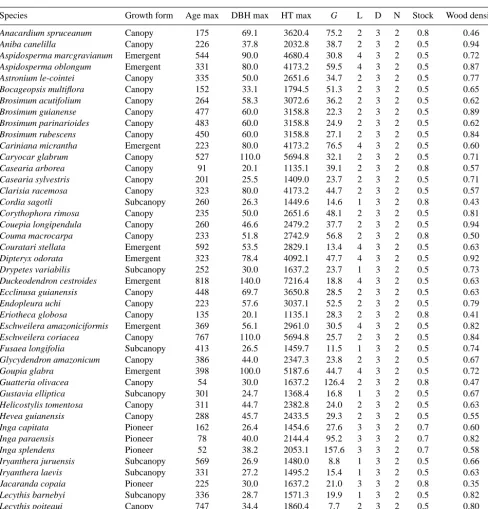
Table 1. Species-specific allometric and ecological parameters for the 90 tree species used in ZELIG-TROP, representing species found in

central Amazonian (Laurance et al., 2004). All species were assigned a probability factor of stress mortality of 0.369, probability factor of natural mortality of 2.813, zone of seed influence of 200, relative seedling establishment rate (RSER) of 0.9, a crown shape value of 4.0, tolerance to drought a ranking of 3, tolerance to low soil nutrients a ranking of 2, minimum growing degree day of 5000, and a maximum growing degree day of 12 229.50.

Species Growth form Age max DBH max HT max G L D N Stock Wood density

Anacardium spruceanum Canopy 175 69.1 3620.4 75.2 2 3 2 0.8 0.46

Aniba canelilla Canopy 226 37.8 2032.8 38.7 2 3 2 0.5 0.94

Aspidosperma marcgravianum Emergent 544 90.0 4680.4 30.8 4 3 2 0.5 0.72

Aspidosperma oblongum Emergent 331 80.0 4173.2 59.5 4 3 2 0.5 0.87

Astronium le-cointei Canopy 335 50.0 2651.6 34.7 2 3 2 0.5 0.77

Bocageopsis multiflora Canopy 152 33.1 1794.5 51.3 2 3 2 0.5 0.65

Brosimum acutifolium Canopy 264 58.3 3072.6 36.2 2 3 2 0.5 0.62

Brosimum guianense Canopy 477 60.0 3158.8 22.3 2 3 2 0.5 0.89

Brosimum parinarioides Canopy 483 60.0 3158.8 24.9 2 3 2 0.5 0.62

Brosimum rubescens Canopy 450 60.0 3158.8 27.1 2 3 2 0.5 0.84

Cariniana micrantha Emergent 223 80.0 4173.2 76.5 4 3 2 0.5 0.60

Caryocar glabrum Canopy 527 110.0 5694.8 32.1 2 3 2 0.5 0.71

Casearia arborea Canopy 91 20.1 1135.1 39.1 2 3 2 0.8 0.57

Casearia sylvestris Canopy 201 25.5 1409.0 23.7 2 3 2 0.5 0.71

Clarisia racemosa Canopy 323 80.0 4173.2 44.7 2 3 2 0.5 0.57

Cordia sagotli Subcanopy 260 26.3 1449.6 14.6 1 3 2 0.8 0.43

Corythophora rimosa Canopy 235 50.0 2651.6 48.1 2 3 2 0.5 0.81

Couepia longipendula Canopy 260 46.6 2479.2 37.7 2 3 2 0.5 0.94

Couma macrocarpa Canopy 233 51.8 2742.9 56.8 2 3 2 0.8 0.50

Couratari stellata Emergent 592 53.5 2829.1 13.4 4 3 2 0.5 0.63

Dipteryx odorata Emergent 323 78.4 4092.1 47.7 4 3 2 0.5 0.92

Drypetes variabilis Subcanopy 252 30.0 1637.2 23.7 1 3 2 0.5 0.73

Duckeodendron cestroides Emergent 818 140.0 7216.4 18.8 4 3 2 0.5 0.63

Ecclinusa guianensis Canopy 448 69.7 3650.8 28.5 2 3 2 0.5 0.63

Endopleura uchi Canopy 223 57.6 3037.1 52.5 2 3 2 0.5 0.79

Eriotheca globosa Canopy 135 20.1 1135.1 28.3 2 3 2 0.8 0.41

Eschweilera amazoniciformis Emergent 369 56.1 2961.0 30.5 4 3 2 0.5 0.82

Eschweilera coriacea Canopy 767 110.0 5694.8 25.7 2 3 2 0.5 0.84

Fusaea longifolia Subcanopy 413 26.5 1459.7 11.5 1 3 2 0.5 0.74

Glycydendron amazonicum Canopy 386 44.0 2347.3 23.8 2 3 2 0.5 0.67

Goupia glabra Emergent 398 100.0 5187.6 44.7 4 3 2 0.5 0.72

Guatteria olivacea Canopy 54 30.0 1637.2 126.4 2 3 2 0.8 0.47

Gustavia elliptica Subcanopy 301 24.7 1368.4 16.8 1 3 2 0.5 0.67

Helicostylis tomentosa Canopy 311 44.7 2382.8 24.0 2 3 2 0.5 0.63

Hevea guianensis Canopy 288 45.7 2433.5 29.3 2 3 2 0.5 0.55

Inga capitata Pioneer 162 26.4 1454.6 27.6 3 3 2 0.7 0.60

Inga paraensis Pioneer 78 40.0 2144.4 95.2 3 3 2 0.7 0.82

Inga splendens Pioneer 52 38.2 2053.1 157.6 3 3 2 0.7 0.58

Iryanthera juruensis Subcanopy 569 26.9 1480.0 8.8 1 3 2 0.5 0.66

Iryanthera laevis Subcanopy 331 27.2 1495.2 15.4 1 3 2 0.5 0.63

Jacaranda copaia Pioneer 225 30.0 1637.2 21.0 3 3 2 0.8 0.35

Lecythis barnebyi Subcanopy 336 28.7 1571.3 19.9 1 3 2 0.5 0.82

Lecythis poiteaui Canopy 747 34.4 1860.4 7.7 2 3 2 0.5 0.80

Table 1. Continued.

Species Growth form Age max DBH max HT max G L D N Stock Wood density

Licania apetala Canopy 199 38.4 2063.3 37.8 2 3 2 0.5 0.76

Licania oblongifolia Canopy 196 54.2 2864.6 65.7 2 3 2 0.5 0.88

Licania octandra Subcanopy 339 35.0 1890.8 21.7 1 3 2 0.5 0.81

Licania cannella Canopy 359 56.5 2981.3 29.0 2 3 2 0.5 0.79

Macrolobium angustifolium Canopy 335 40.0 2144.4 27.7 2 3 2 0.5 0.68

Manilkara bidentata Emergent 773 90.0 4680.4 20.6 4 3 2 0.5 0.87

Manilkara huberi Emergent 349 100.0 5187.6 55.9 4 3 2 0.5 0.93

Maquira sclerophylla Emergent 420 60.0 3158.8 24.0 4 3 2 0.5 0.53

Mezilaurus itauba Canopy 684 44.0 2347.3 12.9 2 3 2 0.5 0.74

Micropholis guyanensis Canopy 248 55.5 2930.6 45.9 2 3 2 0.5 0.66

Micropholis venulosa Canopy 491 60.0 3158.8 22.9 2 3 2 0.5 0.67

Minquartia guianensis Emergent 490 70.0 3666.0 30.4 4 3 2 0.5 0.77

Myrciaria floribunda Subcanopy 490 29.1 1591.6 11.7 1 3 2 0.5 0.77

Onychopetalum amazonicum Canopy 195 29.9 1632.1 33.0 2 3 2 0.5 0.61

Parkia multijuga Emergent 206 119.0 6151.3 101.7 4 3 2 0.8 0.39

Peltogyne paniculata Canopy 251 40.0 2144.4 28.0 2 3 2 0.5 0.80

Pourouma bicolor Pioneer 48 29.8 1627.1 124.6 3 3 2 0.8 0.38

Pourouma guianensis Pioneer 58 31.3 1703.2 112.8 3 3 2 0.8 0.38

Pouteria ambelaniifolia Canopy 296 38.0 2043.0 21.0 2 3 2 0.5 0.70

Pouteria anomala Emergent 452 70.0 3666.0 31.6 4 3 2 0.5 0.78

Pouteria caimito Canopy 240 43.2 2306.7 36.4 2 3 2 0.5 0.82

Pouteria eugeniifolia Canopy 329 44.1 2352.4 25.8 2 3 2 0.5 1.10

Pouteria guianensis Canopy 720 80.0 4173.2 17.5 2 3 2 0.5 0.94

Pouteria macrophylla Canopy 387 29.6 1616.9 13.2 2 3 2 0.5 0.86

Pouteria manaosensis Canopy 981 50.0 2651.6 8.4 2 3 2 0.5 0.64

Pouteria multiflora Canopy 547 35.5 1916.2 9.5 2 3 2 0.5 0.75

Pouteria oppositifolia Canopy 277 35.8 1931.4 21.7 2 3 2 0.5 0.65

Pouteria venosa Canopy 702 45.8 2438.6 10.0 2 3 2 0.5 0.92

Protium altsonii Emergent 238 70.0 3666.0 56.4 4 3 2 0.5 0.68

Protium decandrum Canopy 158 32.8 1779.2 40.3 2 3 2 0.5 0.52

Protium heptaphyllum Canopy 96 26.2 1444.5 60.0 2 3 2 0.8 0.62

Protium tenuifolium Canopy 170 38.2 2053.1 49.1 2 3 2 0.5 0.57

Qualea paraensis Emergent 379 70.0 3666.0 31.9 4 3 2 0.5 0.67

Scleronema micranthum Emergent 353 90.0 4680.4 50.3 4 3 2 0.5 0.60

Sloanea guianensis Subcanopy 179 28.5 1561.1 26.8 1 3 2 0.5 0.82

Swartzia corrugata Subcanopy 407 21.1 1185.8 7.7 1 3 2 0.5 1.06

Swartzia recurva Canopy 177 38.4 2063.3 45.5 2 3 2 0.5 0.97

Swartzia ulei Canopy 293 50.0 2651.6 39.1 2 3 2 0.5 1.00

Tachigali paniculata Canopy 91 27.7 1520.6 60.1 2 3 2 0.8 0.56

Tapirira guianensis Canopy 54 41.6 2225.6 188.0 2 3 2 0.8 0.45

Tetragastris panamensis Canopy 320 38.4 2063.3 25.1 2 3 2 0.5 0.72

Vantanea parviflora Canopy 205 69.6 3645.7 65.1 2 3 2 0.5 0.84

Virola calophylla Subcanopy 293 30.8 1677.8 18.6 3 2 2 0.8 0.51

Virola multinervia Canopy 373 32.0 1738.7 14.0 2 3 2 0.8 0.45

Virola sebifera Canopy 161 30.2 1647.4 44.4 2 3 2 0.8 0.46

Vochysia obidensis Canopy 92 47.4 2519.7 109.1 2 3 2 0.8 0.50

Key: AGEMAX, maximum age for the species (yr); DBH max, maximum diameter at breast height (cm); HT max, maximum height (cm);G, growth-rate scaling coefficient (unitless); light (L): light/shade tolerance class (ranking 1–5); stock, regeneration stocking (%), wood density (g cm−3); (full parameter explanation found in original ZELIG paper: Urban, 1990).

5778 J. A. Holm et al.: Forest response to increased disturbance in the central Amazon

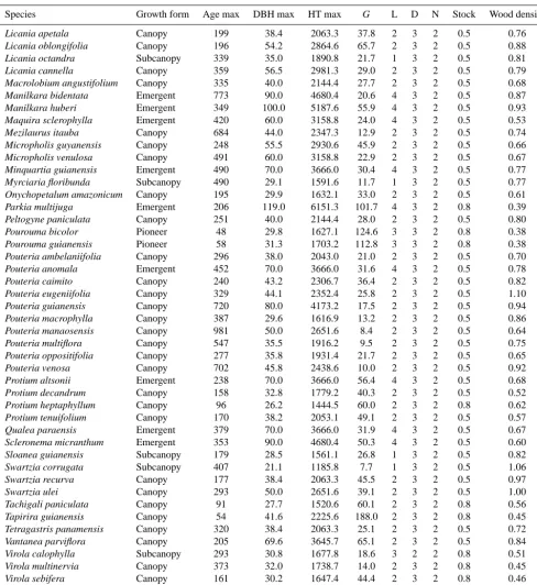
Table 2. Environmental parameters used in ZELIG-TROP for the central Amazon basin. Values reported in a range were monthly low and

high averages.

Lat./long./ Plot Mean monthly Mean monthly Soil field Soil Relative direct alt. (m) area temperature precipitation capacity wilting and diffuse solar

(m2) (◦C) (cm) (cm)a point (cm)a radiation (%)

−2.3/−60.0/ 400.0 25.18–27.47 8.01–45.16 52.0 32.9 0.6/0.4 100.0

a_{Laurance et al. (1999).}

sources with sites across South America (Fearnside, 1997; Chave et al., 2006).

We used results found by Laurance et al. (2004) to deter-mine several parameters; specifically the maximum age of the species (AGEMAX), the maximum diameter at breast height (DBHmax, cm), and the growth-rate scaling coeffi-cient (G) for ZELIG-TROP. AGEMAX was found by tak-ing the mean of three longevity estimates. DBHmax were

scaled to match a more accurate representation of maximum DBH in the simulated field sites (Chambers et al., 2004). We used the canopy classification as described by Laurance et al. (2004) to infer species-specific rankings for tolerance and intolerance to shading. Average monthly precipitation (cm) and temperature (◦C) required for the environmental param-eters in ZELIG-TROP (Table 2) were based on field data col-lected from 2002 to 2004 in the study site (Tribuzy, 2005). Soil field capacity (cm) and soil wilting point (cm) were de-termined from soil measurements in nearby central Amazon study sites (Laurance et al., 1999).

In order to more accurately simulate the central Ama-zonian forest, a few modifications were made to the orig-inal ZELIG-TROP model (Holm et al., 2012). First, the allometric equation used to estimate aboveground biomass (Mg C ha−1) was updated to include an equation specific for the Brazilian rain forest in the central Amazon (Chambers et al., 2001; Eq. 1).

ln(mass)=α+β1ln(DBH)+β2[ln(DBH)]2+β3[ln(DBH)]3, (1)

where aboveground biomass (mass) is in kg,αis−0.370,β1 is 0.333,β2is 0.933, andβ3is−0.122 (r_adj2 =0.973) based upon data collected from 315 harvested trees. Specific wood density is not taken into account in this model.

In model development of the original ZELIG-TROP (mod-ified for a subtropical dry forest), death caused by natural mortality (age-related) was killing tropical trees prematurely. This was also seen in initial model testing for the wet tropical forest. In contrast to tropical dry forests, individuals in tropi-cal wet forests have a longer life potential and a higher likeli-hood of reaching their potential size. For example, the central Amazon is able to support trees>1000 yr old (Chambers et al., 1998, 2001; Laurance et al., 2004), where a dry forest may only be able to support trees to a maximum of 400 yr. To adjust for this variation, the natural survivorship rate was

increased from 1.5 to 6 % of trees surviving to their maxi-mum age (Table 1). This was a conservative value, with one study estimating about 15 % of species in central Amazon at-taining their maximum ages (Laurance et al., 2004). Lastly, we also modified ZELIG-TROP’s mean available light grow-ing factor algorithm, which in part was used to accurately calculate tree height and crown interaction effects, as devel-oped in ZELIG-CFS (Larocque et al., 2011). To best portray tree growth and crown development typical of an individual within a tropical canopy, we used an earlier algorithm ver-sion developed for ZELIG-CFS. This algorithm was the ratio of available growing light factor (ALGF) to a doubled crown width for each individual, thereby adjusting the ALGF rela-tive to horizontal space occupied by the crown and improving the predictive capacities of ZELIG-TROP for the Amazon. This modification thus affected the light extinction on tree growth, allowed more available light from the top to the bot-tom of the individual-tree crown, and in turn better predicted observed data of basal area growth and abundance of stems per plot.

2.2.2 Verification methods

ZELIG-TROP simulations for the central Amazonian for-est were run for 500 yr and replicated on 100 independent plots, each the size of 400 m2. All simulations began from bare ground, and results from ZELIG-TROP were averaged over the final 100 yr of simulation. This was the period when forest dynamics (e.g., stem density, AGB, ANPP) were seen to reach a stable state and represent a mature forest stand. The model was verified by comparing the following five simulated forest attributes (average±SD) to observed field data from the two inventory transects: (1) total basal area (m2ha−1), (2) total AGB (Mg C ha−1), (3) total stem density (ha−1_{), (4) leaf area index, and (5) ANPP (Mg C ha}−1_yr−1_). To test model validity for the central Amazonian forest, we report percent difference between the observed and simulated results (Table 3).

2.3 Disturbance treatments

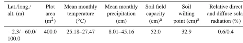
Table 3. Averages (and standard deviations) of five forest attributes for the observed values recorded from sites near Manaus, Brazil, averaged

over 5 ha, and the modeled ZELIG-TROP results. ZELIG-TROP results are averaged for the final 100 yr, after an initial spin up of 400 yr. The remaining values correspond to the percent differences between the observed and simulated values, and the minimum and maximum range of a ZELIG-TROP simulation.

Avg. basal Avg. biomass Avg. stem Avg. LAI Avg. ANPP Area (m2ha−1) (Mg C ha−1) Density (ha−1) (Mg C ha−1yr−1)

Empirical data 30.06 (6.61) 169.84 (27.60) 656 (22) 5.7 (0.50) 6.5 ZELIG-TROP 32.96 (1.22) 178.38 (10.53) 574 (70) 5.8 (0.24) 5.4 (0.22)

Percent diff. (%) 9.66 5.03 −12.49 1.75 −17.08

ZELIG-TROP min./max. 31.14/35.97 167.97/189.26 472/688 5.26/6.48 5.08/5.92

ZELIG-TROP and CLM assuming an independent mecha-nism as the driver of mortality. A description of the Com-munity Land Model (CLM) can be found in the supplemen-tary materials. Predicting the impacts of increased mortality is critical since other recent studies have found that tree mor-tality in the central Amazon has been undersampled in plot-based approaches, and after analyzing a larger range of gap sizes (including larger gaps), ∼9.1 to 16.9 % of tree mor-tality was missing (Chambers et al., 2013). The majority of gaps created in Amazonian rain forests are from windthrow of canopy trees with a large percentage of gaps having rel-atively small areas of<200 m2(Uhl, 1982; Denslow, 1987; Stanford, 1990). However, some windthrow events will cre-ate large gaps that then initicre-ate secondary succession pro-cesses (Brokaw, 1985, Chambers et al., 2013). Since there can be multiple spatial scales and drivers of tree mortal-ity, we are simulating mortality as a stochastic, indepen-dent event within ZELIG-TROP, using the new versatile dis-turbance routine implemented in Holm et al. (2012). Most mortality events in the central Amazon occur on individ-ual trees (Chambers et al., 2004, 2013). Therefore, this phe-nomenon was replicated in the model. Specifically, any one tree >10 cm DBH was randomly selected to die and be re-moved from the forest canopy on an annual basis at the gap scale, in addition to the existing selection of trees removed by natural senescence. This “high-disturbance” treatment for the central Amazonian forests is representative of the cur-rent turnover rates in “west and south” (Phillips et al., 2004), thus creating an opportunity to test whether the variability in forest dynamics and carbon stocks between the “west and south” and the central Amazonian forests can be explained by the variability in the natural disturbance regime. Variables compared between the two regions included AGB, wood density (Baker et al., 2004a), recruitment rates, and stem den-sity (Phillips et al., 2004), and stand-level BA growth rates (Lewis et al., 2004).

A second treatment has been applied in order to improve understanding of periodic large-scale disturbance and re-covery events. This treatment consisted of removing 20 % of stems >10 cm DBH every 50 yr (i.e., periodic treat-ment). It has recently been noted that patch-scale (400 m2)

succession-inducing disturbances exhibit a return frequency of about 50 yr within the central Amazon region (Chambers et al., 2013). Therefore we have set our large-scale distur-bance event to repeat four times over a 200 year period (ev-ery 50 yr) after the forest has reached a mature stable state. This treatment was also conducted in both ZELIG-TROP and CLM. An important metric in determining the forest carbon balance as a result of disturbance is the total change in stand biomass over time (1AGB, Mg C ha−1), defined as AGBt2– AGBt1over the simulation period.

3 Results

3.1 Model verification results

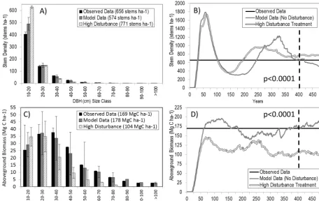
Results simulated by ZELIG-TROP for the mature central Amazon tropical forest (pre-disturbance treatment) were in close range (e.g., within 17 %) to empirical data (Table 3), making ZELIG-TROP successful at predicting stand dynam-ics of a complex tropical forest. Average basal area was 9.7 % higher than the observed value (32.96 vs. 30.06 m2ha−1), av-erage AGB was 5.0 % higher (178.38 vs. 169.84 Mg C ha−1), and average leaf area index (LAI) was 1.8 % higher (5.8 vs. 5.7). ZELIG-TROP predicted average stem density to be 12.5 % lower (574 vs. 656 stems ha−1), and ANPP was 17.1 % lower than observed values reported by Chambers et al. (2001) (5.4 vs. 6.5 Mg C ha−1yr−1). ZELIG-TROP was also successful at accurately predicting stem density and AGB by DBH (cm) size class (Fig. 1a, c). The model over predicted the number of stems in the lowest size class (10–20 cm), by an additional 84 stems per hectare, and in the eighth size class (80–90 cm), but for the remaining size classes values were near to the observed data. Even with these slight over predictions in certain DBH size classes, the model predicted AGB to be within a reasonable range (8.5 Mg C ha−1) of the observed values (r2=0.60).

ZELIG-TROP was also able to predict a realistic commu-nity composition (Fig. 2a). After initiating the model from bare ground, there was a sudden increase in basal area per species, followed by a typical jigsaw pattern of die-offs and growth increases, with the model reaching a steady state

5780 J. A. Holm et al.: Forest response to increased disturbance in the central Amazon

51  

1116  

1117  

Fig. 1.

Comparison between observed field data from “transects” in Central Amazon,

ZELIG-1118  

TROP model data from no-disturbance scenario, and ZELIG-TROP model data from

high-1119  

disturbance treatment.

(A)

Average stem density (stems ha

) and SD by DBH (cm) size class,

(B)

1120  

stem density simulated over 500 years,

(C)

average above-ground biomass (Mg ha

) and SD by

1121  

DBH (cm) size class, and

(D)

above-ground biomass simulated over 500 years. Average results

1122  

and t-test between two model results taken once the model reached a steady-state, or the final 100

1123  

years of simulation.

1124  

Figure 1. Comparison between observed field data from “transects” in central Amazon, ZELIG-TROP model data from no-disturbance

scenario, and ZELIG-TROP model data from high-disturbance treatment. (a) Average stem density (stems ha−1) and SD by DBH (cm) size class, (b) stem density simulated over 500 yr, (c) average aboveground biomass (Mg ha−1) and SD by DBH (cm) size class, and (d) aboveground biomass simulated over 500 yr. Average results andttest between two model results taken once the model reached a steady state, or the final 100 yr of simulation.

during the last 100 yr. The dominant species in terms of basal area, Parkia multijuga, a large, fast-growing emergent species from the Leguminosae family accounted for 17 % of the total basal area in the last 100 yr of simulation. The next four dominant species were all canopy-level species. This was an accurate representation of the forest, as the canopy layer consists of many tree crowns, large trees, and usually a dense area of biodiversity (Wirth et al., 2001). For example, 63 % of the 90 tree species simulated were categorized as a canopy growth form. However, there was also an even mix-ture of emergent, sub-canopy, and pioneer species as domi-nant and rare species, typical of a diverse central Amazonian forest. There was no one single species that dominated the canopy throughout the course of the simulation. Instead, we saw a diverse species representation (Fig. 2a). During the last 100 yr of simulation, emergent species represented 29.6 % of the total basal area, sub-canopy species represented 1.7 %, and pioneer species represented 5.5 % of the total basal area. Empirical mortality rates (% stems yr−1) from BDFFP and BIONTE data were lognormally distributed averag-ing 1.02±1.72 % (Chambers et al., 2004). As estimated by ZELIG-TROP, the no-disturbance annual mortality rates were near to observed values (1.27±0.21 %) but had a

smaller distribution around the mean (Fig. 3). As expected, annual mortality rate doubled (2.66±0.26 %) for the high-disturbance treatment.

3.2 Central and western amazon disturbance comparisons

3.2.1 AGB, stem density, growth and recruitment rates

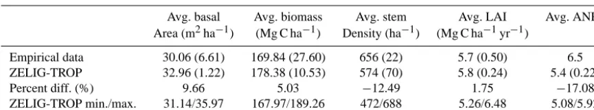
Table 4. Comparison of empirical data and stand model data from Chambers et al. (2004) unless otherwise noted, ZELIG-TROP pre- and

post-disturbance treatments, and CLM pre- and post-disturbance treatments for the pool of carbon in live trees, and the annual flux of carbon from stem growth, coarse litter production rates from mortality, ANPP; and recruitment rate of stems, mean DBH, and average1AGB.

Positive Live Growth Coarse ANPP Recruitment Mean DBH AGB

=sink trees (Mg C ha−1yr−1) litter (Mg C ha−1yr−1) (% yr−1) (cm) change (Mg C ha−1) (Mg C ha−1yr−1) (Mg C ha−1yr−1) Empirical4 156 1.70 −2.10 6.505 1.386 21.1 NA Stand Model4 160 1.60 −1.70 6.60 NA 20.4 NA ZELIG-TROP1 178 3.09 −3.03 5.39 2.33 22.3 0.02 ZELIG-TROP2 104 2.89 −2.78 5.35 3.94 18.3 0.01 ZELIG-TROP3 138 3.29 −3.49 5.06 3.41 26.9 −0.15 CLM-CN1 269 4.88 −4.82 7.81 NA NA 0.04 CLM-CN2 135 4.91 −4.93 7.83 NA NA 0.00 CLM-CN3 230 4.71 −4.95 7.54 NA NA −0.46 ZELIG Diff.1,2 −74 −0.20 0.25 −0.04 1.61 −4.0 0.01 ZELIG Diff.1,3 −40 0.20 −0.46 −0.33 1.08 4.6 −0.17 CLM Diff.1,2 −134 0.03 −0.11 0.02 NA NA −0.04 CLM Diff.1,3 −39 −0.17 −0.15 −0.27 NA NA −0.50

1_{=no disturbance,}2_{=high disturbance,}3_{=periodic disturbance,}4_{Chambers et al. (2004),}5_{Chambers et al. (2001),}6_{Phillips et al. (2004).}

  52  

1125  

1126  

1127  

Fig. 2.(A) Model simulated successional development for all species modeled in ZELIG-TROP

1128  

for a Central Amazon forest, separated by canopy growth form (emergent, canopy, sub-canopy, or

1129  

pioneers). Species composition reported in individual basal area (m2 _ha-1_{). (B) Model simulated}

1130  

successional development for all species modeled in ZELIG-TROP after the high-disturbance

1131  

treatment.

1132  

A) No Disturbance

B) High Disturbance

Figure 2. (a) Model simulated successional development for all

species modeled in ZELIG-TROP for a central Amazonian forest, separated by canopy growth form (emergent, canopy, sub-canopy, or pioneers). Species composition reported in individual basal area (m2ha−1). (b) Model simulated successional development for all species modeled in ZELIG-TROP after the high-disturbance treat-ment.

  53  

1133  

1134  

Fig. 3. Comparison of relative frequency of annual mortality rates (% stems year-1_{) from observed}

1135  

data, ZELIG-TROP no-disturbance, and ZELIG-TROP high-disturbance model data after the

1136  

disturbance treatment. (Observed data: Chambers et al. 2004).

1137  

0.00 0.05 0.10 0.15 0.20 0.25 0.30 0.35

0.1

5

0.3 _0.45 0.6 _0.75 0.9 _1.05 1.2 _1.35 1.5 5 _1.6 1.8 _1.95 2.1 _2.25 2.4 _2.55 2.7 _2.85 3

More

R

el

ati

ve

Fr

eq

ue

nc

y

Mortality Rate (% stems yr-1) Observed Data (1.02%)

ZELIG-TROP No Disturbance (1.27%) ZELIG-TROP High Disturbance (2.66%)

Figure 3. Comparison of relative frequency of annual

mortal-ity rates (% stems yr−1) from observed data, ZELIG-TROP no-disturbance, and ZELIG-TROP high-disturbance model data after the disturbance treatment. (Observed data: Chambers et al., 2004).

set, but there was a significant increase in the model results (Fig. 4).

The high-disturbance treatment did significantly reduce AGB in the central Amazon to values similar to the “west and south” counterpart, but wood density was not included in the biomass allometric equation for the central Amazon there-fore this reduction in AGB was a “false-positive”. Specif-ically, when the central Amazon was subjected to faster turnover rates there was a significant reduction in AGB (two sample t test, t(99,1.97)=108.98, p <0.001) and net

car-bon loss was 74 Mg C ha−1(from 178 to 104 Mg C ha−1) av-eraged over the last 100 yr of simulation (Fig. 1d) equiv-alent to a 41.9 % decrease. AGB in the central Amazon

5782 J. A. Holm et al.: Forest response to increased disturbance in the central Amazon

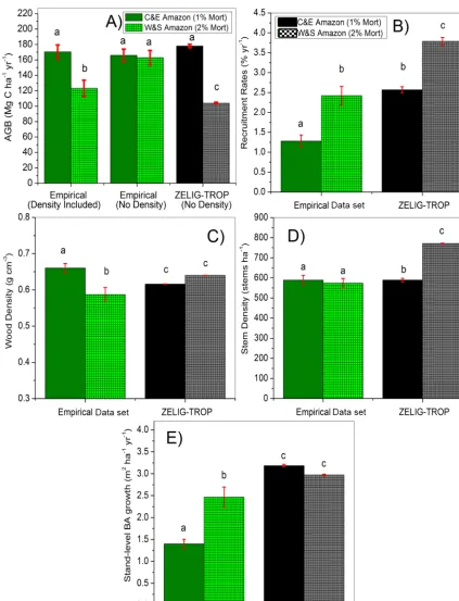
Figure 4. Comparison between “central and eastern” Amazon (“slow dynamics”) and “west and south” Amazon (“fast dynamics”)

be-tween the empirical (RAINFOR data set, green columns) and modeled ZELIG-TROP results for average (a) aboveground biomass (AGB, Mg C ha−1yr−1) with the observed data set either including or not including wood density in the Chambers et al. (2001) allometric equation,

55  

1147  

Fig. 5

. CLM-CN model evaluation and comparisons to ZELIG-TROP for a no-disturbance

1148  

scenario and a high disturbance treatment:

(A)

ANPP,

(B)

above-ground biomass,

(C)

stem

1149  

growth,

(D)

coarse litter production rates, all measured in Mg C ha

, and

(E)

basal area from

1150  

ZELIG-TROP and observed data in green as reported by Baker et al. (2004a), and

(F)

leaf area

1151  

index (LAI) from CLM-CN4.5 and observed data in green as reported by McWilliams et al.

1152  

(1993) and Malhi et al. (2013). Statistical significance test in all panels are two-sample Student’s

1153  

t-test between the no-disturbance and high disturbance treatments, separately for each model.

1154  

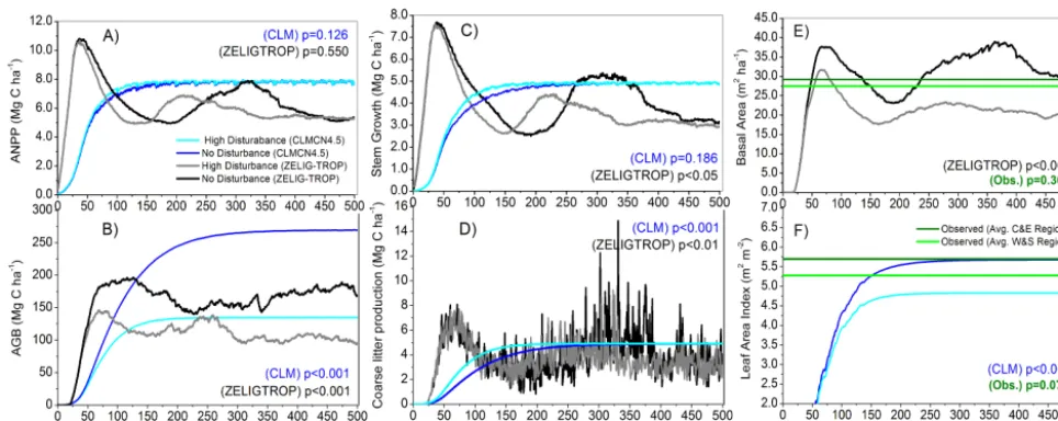
Figure 5. CLM-CN model evaluation and comparisons to ZELIG-TROP for a no-disturbance scenario and a high-disturbance treatment: (a)

ANPP, (b) aboveground biomass, (c) stem growth, (d) coarse litter production rates, all measured in Mg C ha−1, and (e) basal area from ZELIG-TROP and observed data in green as reported by Baker et al. (2004a), and (f) leaf area index (LAI) from CLM-CN4.5 and observed data in green as reported by McWilliams et al. (1993) and Malhi et al. (2013). Statistical significance test in all panels are two-sample Student’sttest between the no-disturbance and high-disturbance treatments, separately for each model.

was impacted the most by the high-disturbance treatment. The AGB from the higher disturbed central Amazon was similar (104 Mg C ha−1) to AGB values in the “west and south” RAINFOR network plots, but only when compar-ing to biomass equations that included weightcompar-ing for wood density (Chave et al., 2001; Chambers et al., 2001). For ex-ample, AGB predicted by the Chave et al. (2001) equation (107 Mg C ha−1_{) had no significant difference between the} two disturbed regions (two sample t test, t(38,2.7)=2.29,

considering alpha=0.01, p=0.03) (Fig. 4a). The signifi-cant reduction in stand basal area, and not variation in wood density, was the main driver of decrease in AGB in ZELIG-TROP (Fig. 5e). However, there was no significant difference in stand basal area between the empirical data sets in the cen-tral and “west and south” plots (p=0.368), a finding also confirmed by Baker et al. (2004a) and Malhi et al. (2006). While net carbon loss was the expected result, it constitutes a “false positive” resulting from omitting wood density in the model estimate of biomass and from an absence of signifi-cant difference in stand basal area across the Amazonia field network.

The high-disturbance treatment in the central Amazon led to a significant increase in stem density by 197 stems from 574 to 771 stems ha−1_{(34.3 % increase, Fig. 1b, two} sample t test, t(99,1.97)= 28.06, p <0.001). Compared

to the regional gradient in the RAINFOR network there was no significant difference between the higher disturbed and the central Amazon empirical data set (573 stems ha−1 vs. 589 stems ha−1) (two sample t test, t(46,2.01)= 0.84,

p=0.4077, Fig. 4d). ANPP did not significantly alter in the central Amazonian forest under a high-disturbance treatment

(two sample t test, t(99,1.97)= 1.54, p=0.1260), only

de-creasing ANPP by 0.04 (from 5.39 to 5.35 Mg C ha−1yr−1, 1.0 %, Fig. 5a). Even with increased disturbance events, ANPP did not decrease in the same manner as biomass due to recovery episodes from more frequent thinning and the increase in smaller stems (i.e., 10 cm DBH size class) in newly opened gaps. When comparing the stand-level BA growth rates (proxy for productivity) in the RAINFOR net-work there was a significant increase in growth rates in the “west and south” compared to the central Amazon, but there was no significant difference between the modeled treat-ments. In fact, an opposite response was seen, and there was a slight decrease as a result of higher disturbance (by 0.21 m2ha−1yr−1, Fig. 4e or 0.20 Mg C ha−1yr−1, Fig. 5c). The model might be inaccurately representing growth rates because prior to applying a higher disturbance regime in the central Amazon, ZELIG-TROP significantly over-estimated the stand-level growth compared to empirical data (3.2 vs. 1.4 m2ha−1yr−1).

The recruitment rates (% yr−1) from the treatment site constitute the only variable that matched the “west and south” observational data set. Under a high-disturbance treat-ment in the central Amazon, as expected, there were subse-quent increases in recruitment rate, where recruitment sig-nificantly increased from 2.3 to 3.9 % yr−1, constituting a 69.1 % increase above no-disturbance recruitment rates (Ta-ble 4, Fig. 6a). Pre-treatment, modeled recruitment rates were 0.9 % yr−1 higher compared to empirical values from the central Amazon BDFFP plots (Phillips et al., 2004). Recruit-ment and mortality rates are tightly linked (Lieberman et al., 1985); therefore, when tree mortality increased, recruitment

5784 J. A. Holm et al.: Forest response to increased disturbance in the central Amazon

56  

1155  

1156  

Fig. 6

.

(A)

Relationship between above-ground biomass (Mg ha

) and recruitment rates (% yr

).

1157  

(B)

Relationship between above-ground biomass (Mg ha

) and coarse litter production rates as a

1158  

result of tree mortality (Mg C ha

yr

), during a no-disturbance, high disturbance, and periodic

1159  

disturbance simulation in ZELIG-TROP for the last 100 years of simulation.

1160  

A)  

B)  

Figure 6. (a) Relationship between aboveground biomass (Mg ha−1) and recruitment rates ( % yr−1). (b) Relationship between above-ground biomass (Mg ha−1) and coarse litter production rates as a result of tree mortality (Mg C ha−1yr−1), during a no-disturbance, high-disturbance, and periodic disturbance simulation in ZELIG-TROP for the last 100 yr of simulation.

also significantly increased. In the “west and south” em-pirical data set recruitment rates were ∼79 % higher com-pared to the central region (Fig. 4b). However, while turnover rates increased, there was not an increase in coarse litter production rate (trunks and large stems >10 cm diameter, Mg C ha−1yr−1, Fig. 6b) compared to the no-disturbance scenario, but rather a significant decrease (two samplettest,

t(99,1.97)=2.70,p <0.01). Under a high-disturbance

treat-ment, the production of coarse litter decreased by an average of 0.25 Mg C ha−1_yr−1 _{(8.3 %, Table 4). However, it is} un-clear if this decrease in production of coarse litter is biologi-cally or atmospheribiologi-cally significant.

Once the forest reached a mature stable state (after 500 yr) the periodic disturbance treatment was applied, removing 20 % of stems in the mature forest every 50 yr (for a du-ration of 200 yr). The carbon loss over the 200 yr period, including the four large-scale disturbances, was less severe than the high-disturbance treatment, but was still a significant decrease (two sample t test, t(99,1.97)=22.73,p <0.001).

Compared to the no-disturbance scenario, average AGB net carbon loss was 40 Mg C ha−1(from 178 to 138 Mg C ha−1, 22.7 %, Fig. 7c) and ANPP significantly decreased from an average of 5.39 to 5.06 Mg C ha−1_yr−1_{(6.1 %, two samplet} test,t(99,1.97)=7.65,p <0.001). For the periodic treatment,

the decrease in biomass was roughly half the decrease ob-served in the high-disturbance treatment; however, the de-crease in ANPP was more severe.

3.3 Community composition changes

The individual-based dynamic vegetation model approach was able to explore the long-term changes to community composition and fate of each species with increased

distur-bance. A high-disturbance treatment shifted species compo-sition towards a more even canopy structure, and increased the species evenness and diversity (Fig. 2b). The largest basal area reduction occurred in the most common species; specif-ically the top two emergent species, followed by the most common canopy species. With an increase in disturbance, the species originally occupying the largest basal area on the plot, Parkia multijuga, decreased by 94.8 % in relative differ-ence in basal area compared to all species averaged over the last 100 yr. The next most common emergent species, Carini-ana micrantha, decreased by 32.6 % with high disturbance, and canopy species filled in as the dominant growth form (Fig. 2b).

57  

1162  

Fig. 7

. CLM-CN model evaluation and comparisons to ZELIG-TROP for a periodic disturbance

1163  

treatment:

(A)

ANPP,

(B)

stem growth,

(C)

aboveground biomass (AGB), and

(D)

coarse litter

1164  

production rates, all measured in Mg C ha

. Statistical significance test in all panels are

two-1165  

sample Student’s t-test between the no-disturbance and high disturbance treatments, separately for

1166  

each model.

1167  

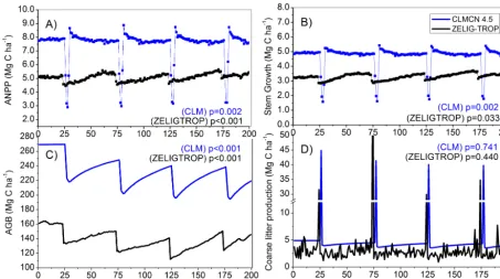
Figure 7. CLM-CN model evaluation and comparisons to ZELIG-TROP for a periodic disturbance treatment: (a) ANPP, (b) stem growth, (c) aboveground biomass (AGB), and (d) coarse litter production rates, all measured in Mg C ha−1. Statistical significance test in all panels are two-sample Student’sttest between the no-disturbance and high-disturbance treatments, separately for each model.

wood density would decrease, as expected in a forest with higher turnover rates. However, the dominant species prior to disturbance (the emergent: Parkia multijuga), which experi-enced the largest decrease in basal area, had a very low wood density (0.39 g cm−3). In addition, even though the emergent size class decreased, the canopy species (which also had high average wood density of 0.71 g cm−3) basal area increased from 63 % to 79.6 %, and the increase in pioneer species from 5.5 % to 5.9 % was not sufficient to lower the total wood den-sity of the forest. With higher disturbance rates subcanopy species represented 6.7 % of the total basal area, compared to 1.7 % prior to high disturbances.

3.4 Disturbances and carbon change in CLM-CN 4.5 vs. ZELIG-TROP

After applying a continual disturbance regime within CLM as in ZELIG-TROP, similar patterns in forest biomass in response to disturbance were observed, and both models were in agreement with each other. For example, the relative change in AGB was consistent (41.9 % vs. 49.9 % decrease) for ZELIG-TROP and CLM, respectively (Fig. 5b). In CLM the aboveground carbon storage pools are not determined us-ing allometric equations, but rather through a carbon alloca-tion framework based off of photosynthesis, total GPP, and respiration (Thornton et al., 2002). Including or excluding specific wood density is not considered in CLM. The model outputs from CLM for the disturbed central Amazon also

showed a reduction in AGB similar to the “west and south”; which was also a “false-positive” result. The significant loss of LAI with disturbance was the main driver of reduction in AGB (Fig. 5f). There was a weak non-significant differ-ence in LAI between the empirical data sets in the central and “west and south” Amazon regions (p=0.077). Another similarity between the two models was the non-significant change in ANPP; however, ZELIG-TROP predicted a de-crease in ANPP while CLM predicted a slight inde-crease in ANPP (Fig. 5a).

With regards to the periodic disturbance treatment of large-scale disturbance events, CLM also replicated analo-gous patterns in biomass loss and recovery as seen in ZELIG-TROP (Fig. 7c). In both models, the sudden decrease in biomass as well as re-equilibration during the recovery phase matched. During each pulse disturbance, the forest lost on av-erage 18.3 and 18.7 % biomass in ZELIG-TROP and CLM, respectively, and gained 16.5 and 15.4 % biomass during the recovery phase. Both CLM and ZELIG-TROP predicted that the recovering forest biomass, on average, was less than the amount lost in each large-scale disturbance event, therefore generating a negative total1AGB (−0.15 and -0.46 Mg C ha−1yr−1 for ZELIG-TROP and CLM, respec-tively, Table 4). The negative total1AGB was less in ZELIG-TROP, and was likely attributed to ZELIG-TROP predict-ing growth rates to significantly increase (by 0.20 Mg C ha−1 yr−1, two sample t test, t(99,1.97)=2.14, p <0.05), most

likely due to the open gaps from disturbance; therefore,

5786 J. A. Holm et al.: Forest response to increased disturbance in the central Amazon

losses were damped in ZELIG-TROP. In contrast CLM had growth rates that on average decreased, due to the sharp de-crease in growth rates following each large-scale disturbance event (Fig. 7b). Both models also showed that each subse-quent recovery period was always greater than the previous period, up to a point where re-growth matched the biomass lost in the disturbance event (Fig. 7c).

There were discrepancies with the response of ANPP to the periodic large-scale forest mortality and recovery events between CLM and ZELIG-TROP. The immediate decrease in ANPP following the large-scale disturbance event was significantly greater in CLM compared to ZELIG-TROP (4.7 vs. 0.6 Mg C ha−1yr−1, Fig. 7a). The subsequent shape of ANPP during the 50 yr recovery was also different be-tween the two models. CLM predicted that within approx-imately two years after the disturbance, ANPP returned to pre-disturbance levels and stayed relatively constant until the next disturbance. However, ZELIG-TROP did not display a fast return to pre-disturbance levels, but instead predicted a gradual increase in ANPP after each disturbance. Comparing the no-disturbance scenario and the periodic treatment, both models predicted that overall ANPP significantly decreased with periodic disturbances (two samplettest,p <0.001 and

p=0.002 for ZELIG-TROP and CLM, respectively); how-ever, the gap model predicted a greater percent difference in average ANPP; a 6.1 % decrease vs. 3.5 % decrease in CLM. To answer our last research question, what are the dif-ferences after increasing disturbance rates in ZELIG-TROP vs. CLM for the central Amazon, we did find other discrep-ancies. While the magnitude of change between AGB was similar between the two models, CLM differs greatly from ZELIG-TROP in that it did not captured the inter-annual vari-ability in carbon stocks, while ZELIG-TROP did (Fig. 5b). Therefore, the demographic forest model captured large fluc-tuations in annual forest biomass and carbon stocks as a sult of either gap dynamics, changes in competition for re-sources, and/or varying size class and age class structure of the forest. In addition, CLM did not produce pulses of coarse litter in response to tree mortality representative of a hetero-geneous landscape (Figs. 5d, 7d). While the relative change in AGB was consistent between the two models, there was a large overestimation in the absolute values. With the inclu-sion of the high-disturbance treatment CLM predicted that average AGB net carbon loss was 134 Mg C ha−1(from 269 to 135 Mg C ha−1) vs. 74 Mg C ha−1in ZELIG-TROP.

4 Discussion

4.1 Elevated forest disturbance and long-term impacts Disturbance is likely to increase in Amazonian forests. Since the mid-1970s observed tree mortality and recruitment rates have been increasing in the Amazon (Phillips et al., 2004), and higher than usual mortality rates have also been

associ-ated with droughts and strong windstorm events (Nepstad et al., 2007; Chambers et al., 2009; Phillips et al, 2009; Negrón-Juárez et al., 2010; Lewis et al., 2011), each of which could increase with human-induced climate change. In addition, re-ported mortality rates might be underestimated as 9.1–16.9 % of tree mortality was missing from plot-based estimates in the Amazon (Chambers et al., 2013). We first investigated the impact of continual high disturbance (100 yr) in a cen-tral Amazonian forest using a demographic forest model as a benchmark model due to operating at finer scales and having mechanistic mortality algorithms. The elevated disturbance resulted in a decrease in AGB by 41.9 %, with essentially no change in ANPP (1.0 % decrease), and an increase in re-cruitment rates by 69.1 %. As a result of higher proportion of smaller stems (20.7 % increase in the 10–30 cm DBH size classes), and decrease in large stems, there was a significant decrease in coarse litter production rate of 8.3 %.

We compared empirical data from the higher disturbed “west and south” Amazon plots (“fast dynamics”), to the modeled central Amazonian forest with mirrored tree mor-tality to evaluate if the models used in this study could pre-dict similar forest dynamics and characteristics. Only one at-tribute that is tightly linked with disturbances (i.e., increase in recruitment) followed the same pattern when shifting from low disturbance to high disturbance. The models were not successful in predicting the shift in growth rates and spe-cific wood density; forest processes and traits that have been shown to differ with varying turnover rates (Baker et al., 2004a; Lewis et al., 2004; Phillips et al., 2004). Therefore, results showed that the disturbance regime alone might not explain all of the differences in forest dynamics between the two regions, or the models do not accurately capture all dis-turbance and recovery processes. Furthermore, the net loss in biomass was assumed to be a “false-positive” in the mod-els because in ZELIG-TROP AGB loss was driven by basal area loss, and in CLM AGB loss was driven by LAI loss. Basal area and LAI are not found to be drivers of AGB loss, or patterns of biomass, in empirical data sets (Baker et al., 2004a; Malhi et al., 2006). In contrast basal area var-ied only slightly across the Amazon plot network (27.5 vs. 29.9 m2ha−1, Baker et al., 2004a). This indicates that wood density, which is a strong indicator of functional traits (Whit-more, 1998); along with patterns of family composition are strong drivers in steady-state AGB variation.

the temporal variability in coarse litter inputs, and instead re-mained constant over time. We also compared the response of large-scale periodic disturbances in the two models, and found that CLM captured similar disturbance and recovery patterns as the gap model.

After applying continual and periodic higher disturbance treatments, we did not observe a continual decrease in for-est structure or biomass that lead to a new forfor-est succes-sional trajectory. Instead, we found that the Amazonian for-est shifted to a new equilibrium state. The outcome of a con-tinual higher disturbance rate generated a stable forest but with less biomass, faster turnover, higher stem density con-sisting of smaller stems, as well as less emergent species, less ANPP, and less contribution of coarse litter inputs. In-ventory studies have reported that with increased turnover, there is a change in community composition, less wood den-sity, and when these traits are taken into account there is also less AGB (Baker et al., 2004a). We conclude that including wood density in dynamic vegetation models is needed. While we have shown that terrestrial biomass will decrease with in-creased disturbances, the interacting effects from potential CO2fertilization should be explored.

4.2 Disturbance, biomass accumulation, and CO2fertilization

Demographic vegetation models are useful tools at predict-ing long-term temporal trends related to changes in carbon stocks and fluxes. The offsetting interactions between possi-ble CO2fertilization and disturbances are an important next step to evaluate. Based on observational studies from per-manent plots there has been an increase in tree biomass in Amazonian forests by∼0.4–0.5 t C yr−1_{over the past three} decades (Lewis et al., 2004; Phillips et al., 1998, 2008). CO2 fertilization effects might be an explanation (Fan et al., 1998; Norby et al., 2005), but this is unknown or refuted (Canadell et al., 2007, Norby et al., 2010), and manipulation experi-ments of enhanced CO2 in the tropics is untested (Zhou et al., 2013). Due to the magnitude of forest growth, CO2 fer-tilization may not be a causal factor but instead driven by interacting agents such as biogeography and changing en-vironmental site conditions (Lewis et al., 2004; Malhi and Phillips, 2004). The role of widespread recovery from past disturbances still needs to be explored as an explanation for biomass accumulation.

In a study evaluating the risk of Amazonian forest dieback, Rammig et al. (2010) used rainfall projections from 24 GCMs and a dynamic vegetation model (LPJmL) and pre-dicted that Amazonian forest biomass is increasing due to strong CO2 fertilization effects (3.9 to 6.2 kg C m−2), and outweighs the biomass loss due to projected precipitation changes; however, larger uncertainties are associated with the effect of CO2compared to uncertainties in precipitation. In-creasing evidence from an ensemble of updated global cli-mate models are predicting that tropical forests are at a lower

risk of forest dieback under climate change, in that they can still retain carbon stocks until 2100 due to fertilization ef-fects of CO2 (Cox et al., 2013; Huntingford et al., 2013); however, there is still large uncertainties between models and how tropical forests will respond to interacting effects of increasing CO2 concentrations, warming temperatures, and changing rainfall patterns (Cox et al., 2013).

In this study over the period of 100 yr there was no signif-icant change in biomass accumulation in both ZELIG-TROP and CLM (Fig. 5b), and the forest did not act as a carbon sink as predicted by empirical studies across a network of Ama-zon inventory plots (Phillips et al., 1998, 2004). One expla-nation could be due to atmospheric CO2being held constant. Upon applying the disturbance treatment, the forest became more stable. With regards to periodic disturbances and sud-den tree mortality events, both models predicted a negative

1AGB,−0.15 and−0.46 Mg C ha−1_yr−1_{for ZELIG-TROP} and CLM, respectively; therefore, the forest acted as a carbon source (Table 4). CLM predicted a larger decrease in biomass under periodic disturbances, which offsets the current ob-served biomass accumulation (lower empirical estimates at 0.20–0.39 Mg C ha−1yr−1, Phillips et al., 1998; Chambers and Silver, 2004).

4.3 Lessons learned from modeling tropical forest disturbance

4.3.1 Model comparison to field data and additional sites

We found that using a dynamic vegetation gap model that operates at the species level was successful at replicating the central Amazonian forest. ZELIG-TROP has also been vali-dated for the subtropical dry forest of Puerto Rico (Holm et al., 2012), but this is the first application of a dynamic veg-etation model of this kind (i.e., gap model) for the Amazon Basin. As a result of using species-specific traits, the values reported by ZELIG-TROP for average basal area, AGB, stem density, LAI, and ANPP were all close to observed values (e.g., ranging from 1.7 to 17.1 % difference between ZELIG-TROP and observed field results). Field measurements of AGB from the central Amazon transects averaged (±SD): 169±27.6 Mg C ha−1, and additional field-based measure-ments from nearby sites in the central Amazon (FLONA Tapajós plots) range from 132 to 197 Mg C ha−1 (Miller et al., 2003; Keller et al., 2001). ZELIG-TROP predicted very similar estimates of AGB: 178±10.5 Mg C ha−1_{; therefore,} model results were within the expected range. From a single-point grid cell, located in the same latitude and longitude co-ordinates as observational plots, CLM predicted higher lev-els of AGB (269 Mg C ha−1). In a study comparable to ours, Chambers et al. (2004) found that upon doubling turnover rates in an individual-based stand model, forest biomass for a central Amazonian forest decreased by slightly more than 50 %. This decrease in forest biomass was similar to the

5788 J. A. Holm et al.: Forest response to increased disturbance in the central Amazon

response reported in this study (41.9 and 49.9 %). Unlike the Chambers et al. (2004) study, we did not impose an increase in growth rates in the model parameters in conjunction with elevated turnover rates. Instead, annual growth rates were de-termined internally within ZELIG-TROP based on species-specific parameters and environmental conditions.

4.3.2 Growth rates and wood density

Our prediction of average growth rate was higher than field data found in the central Amazon BDFFP inventory plots (3.1 vs. 1.7 Mg C ha−1yr−1, Table 4), but similar to other values found in the central and eastern Amazon. For example, us-ing a process-based model, Hirsch et al. (2004) found above-ground stem growth to be 3.6 Mg C ha−1yr−1, and field mea-surements were 2.9 Mg C ha−1_yr−1_{at the Seca Floresta site} in the Tapajós National Forest (Rice et al., 2004). During the high-disturbance treatment, we did not observe an increase in average growth rates compared to the no-disturbance treat-ment. In fact, there was a slight decrease in annual growth (Table 4, Fig. 4e). This non-significant change in growth rates could have been due to the non-occurrence of large increases in available light and resources after each additional death, a result of a continual disturbance treatment as opposed to a dramatic disturbance event. Alternatively, the western Ama-zon plots, counterparts to the high-disturbance treatment, did exhibit an increase in growth rates (Fig. 4e). Differences in environmental gradients between regions, such as higher total phosphorous, less weathered, and more fertile soils in the western Amazon (Quesada et al., 2010), could be a stronger controlling factor. In the periodic disturbance treat-ment, growth and productivity did increase directly following each large-scale disturbance (i.e., removing 20 % of stems). After each pulse disturbance ANPP increased by 14 % over the 50-year recovery phase. The change in community com-position under the high-disturbance treatment was also repre-sentative of what would be expected (i.e., emergent species decreased by the largest percent in basal area, and canopy and subcanopy species increased); however, by not captur-ing expected changes in wood density the model might be missing some shifts in species composition in response to disturbance.

Wood density is a robust indicator of life history strategies, growth rates, and/or successional status of a forest (Whit-more, 1998; Suzuki, 1999; Baker et al., 2004a). Upon model-ing a central Amazonian forest with disturbance rates similar to the “west and south”, the higher disturbance did not create a community composition dominated by pioneer species or lower the average wood density, but instead created a forest of less emergent species, more canopy species, and higher wood density. Our results further confirm that environmental and/or stand factors explain the regional variation of AGB and wood density. Even with elevated disturbance in the cen-tral Amazon, the species that persisted and increased in basal area had on average high wood density (0.7 g cm−3). The

growth-rate scaling coefficients, G, used in ZELIG-TROP were inversely correlated with wood density, matching the robust signal observed from inventory data, but was not cor-related (r2=0.13), leading to a possible explanation of the opposite pattern in wood density shifts with increased dis-turbance. Wood density is not a main parameterization vari-able in ZELIG-TROP, and other factors in the gap model (e.g., drought or light tolerances, maximum age, availability of light) could be a stronger driver of community composi-tion shifts over wood density.

It should be noted that wood density is difficult to mea-sure accurately in the field, varies between and within species (Chave et al., 2006), varies within a tree across diameter and from the base of the tree to the top (Nogueira et al., 2005), and the Chambers et al. (2001) AGB model with-out wood density shows that variation of the data explained by the model is strong (r2=0.973). Including wood density in AGB allometric equations is not required, but it is ben-eficial for accounting for differences in carbon stocks due to changes in species composition, gradients in soil fertility (Müller-Landau, 2004) as opposed to disturbance regimes, and can be a key variable in greenhouse gas emission mitiga-tion programs.

4.3.3 CLM 4.5 vs. dynamic vegetation model

Simulating vegetation demography is beneficial to tracking community shifts, plant competition, and dynamic changes in carbon stocks and fluxes, and should be considered be-ing incorporated into CLM. The version of CLM used here does not take into account differences between plant size, plant age, or all biotic and abiotic stressors. Using demog-raphy typical of a gap model will account for these missing factors, will aid in capturing annual carbon variability as a re-sult of heterogeneous mortality across the landscape, and can help improve global land surface models. The exact causes and processes leading to plant mortality are difficult to quan-tify (Franklin et al., 1987; McDowell et al., 2008, 2011), and additional field research is required in this area, especially in the tropics. However, the gap model approach can quan-tify the contribution due to natural death, stress related death, or disturbance related death under no-disturbance and high-disturbance scenarios.