2
Chapter
E
xponential functions are used to model
situations in which growth or decay change
dramatically. Such situations are found in
nuclear power plants, which contain rods of
plutonium-239; an extremely toxic radioactive
isotope.
Operating at full capacity for one year, a 1,000
megawatt power plant discharges about 435 lb of
plutonium-239. With a half-life of 24,400 years,
how much of the isotope will remain after 1,000
years? This question can be answered with the
mathematics covered in Section 1.3.
Chapter 1 Overview
This chapter reviews the most important things you need to know to start learning
calcu-lus. It also introduces the use of a graphing utility as a tool to investigate mathematical
ideas, to support analytic work, and to solve problems with numerical and graphical
meth-ods. The emphasis is on functions and graphs, the main building blocks of calculus.
Functions and parametric equations are the major tools for describing the real world in
mathematical terms, from temperature variations to planetary motions, from brain waves
to business cycles, and from heartbeat patterns to population growth. Many functions
have particular importance because of the behavior they describe. Trigonometric
func-tions describe cyclic, repetitive activity; exponential, logarithmic, and logistic funcfunc-tions
describe growth and decay; and polynomial functions can approximate these and most
other functions.
Lines
Increments
One reason calculus has proved to be so useful is that it is the right mathematics for
relat-ing the rate of change of a quantity to the graph of the quantity. Explainrelat-ing that
relation-ship is one goal of this book. It all begins with the slopes of lines.
When a particle in the plane moves from one point to another, the net changes or
increments
in its coordinates are found by subtracting the coordinates of its starting point
from the coordinates of its stopping point.
Section 1.1 Lines 3
1.1
What you’ll learn about
• Increments
• Slope of a Line
• Parallel and Perpendicular Lines
• Equations of Lines
• Applications
. . . and why
Linear equations are used
exten-sively in business and economic
applications.
The symbols
x
and
y
are read “delta x” and “delta y.” The letter
is a Greek capital
d
for “difference.” Neither
x
nor
y
denotes multiplication;
x
is not “delta times x” nor
is
y
“delta times y.”
Increments can be positive, negative, or zero, as shown in Example 1.
EXAMPLE 1
Finding Increments
The coordinate increments from
4,
3
to (2, 5) are
x
2
4
2,
y
5
3
8.
From (5, 6) to (5, 1), the increments are
x
5
5
0,
y
1
6
5.
Now try Exercise 1.Slope of a Line
Each nonvertical line has a slope,
which we can calculate from increments in coordinates.
Let L
be a nonvertical line in the plane and P
1(x
1,
y
1) and P
2(x
2,
y
2) two points on L
(Figure 1.1). We call
y
y
2y
1the
rise
from P
1to P
2and
x
x
2x
1the
run
from
xy
O
P1(x1, y1)
L
P2(x2, y2)
Q(x2, y1)
x run
y rise
Figure 1.1 The slope of line Lis
m r
r i u
s n e
yx.
DEFINITION
Increments
If a particle moves from the point (x
1,
y
1) to the point (x
2,
y
2), the
increments
in its
coordinates are
P
1to P
2. Since L
is not vertical,
x
0 and we define the slope of L
to be the amount of
rise per unit of run. It is conventional to denote the slope by the letter m.
A line that goes uphill as x
increases has a positive slope. A line that goes downhill as x
increases has a negative slope. A horizontal line has slope zero since all of its points have
the same y-coordinate, making
y
0. For vertical lines,
x
0 and the ratio
y
x
is
undefined. We express this by saying that vertical lines have no slope.
Parallel and Perpendicular Lines
Parallel lines form equal angles with the x-axis (Figure 1.2). Hence, nonvertical parallel
lines have the same slope. Conversely, lines with equal slopes form equal angles with the
x-axis and are therefore parallel.
If two nonvertical lines L
1and
L
2are perpendicular, their slopes m
1and
m
2satisfy
m
1m
21, so each slope is the negative reciprocal
of the other:
m
1m
1
2
,
m
2m
1
1
.
The argument goes like this: In the notation of Figure 1.3,
m
1tan
f
1a
h, while
m
2tan
f
2h
a.
Hence,
m
1m
2(a
h)(
h
a)
1.
Equations of Lines
The vertical line through the point (a,
b) has equation x
a
since every x-coordinate on
the line has the value a.
Similarly, the horizontal line through (a,
b) has equation y
b.
EXAMPLE 2
Finding Equations of Vertical and Horizontal Lines
The vertical and horizontal lines through the point (2, 3) have equations x
2 and
y
3, respectively (Figure 1.4).
Now try Exercise 9.We can write an equation for any nonvertical line L
if we know its slope m
and the
coordinates of one point P
1(x
1,
y
1) on it. If P(x,
y) is any
other point on L, then
y
x
y
x
1 1m,
so that
y
y
1m(x
x
1)
or
y
m(x
x
1)
y
1.
L1x
1 Slope m1
L2
Slope m2
m1
θ1
1
m2
θ2
Figure 1.2 If L1L2, then u1u2and m1m2. Conversely, if m1m2, then u1u2and L1L2.
x y
A D a B
h C L2
1
1
2
Slope m1 Slope m2
L1
O
Figure 1.3 ADCis similar to CDB. Hence f1is also the upper angle in CDB, where tanf1a
h.Along this line,
x 2.
x y
0 1 2 3 4 (2, 3)
1 3
2 4 6
5
Along this line,
y 3.
Figure 1.4 The standard equations for the vertical and horizontal lines through the point (2, 3) are x2 and y3. (Example 2)
DEFINITION
Slope
Let P
1(x
1,
y
1) and P
2(x
2,
y
2) be points on a nonvertical line,
L.
The
slope
of L
is
m
r
r
i
u
s
n
e
y
x
x
y
22
y
x
1 1
.
DEFINITION
Point-Slope Equation
The equation
y
m(x
x
1)
y
1Section 1.1 Lines 5
EXAMPLE 3
Using the Point-Slope Equation
Write the point-slope equation for the line through the point (2, 3) with slope
3
2.
SOLUTION
We substitute x
12,
y
13, and m
3
2 into the point-slope equation and obtain
y
3
2
x
2
3
or
y
3
2
x
6.
Now try Exercise 13.
The
y-coordinate of the point where a nonvertical line intersects the y-axis is the
y
-intercept
of the line. Similarly, the x-coordinate of the point where a nonhorizontal line
intersects the x-axis is the
x
-intercept
of the line. A line with slope m
and
y-intercept
b
passes through (0,
b) (Figure 1.5), so
y
m
x
0
b,
or, more simply,
y
mx
b.
x y
y = mx + b
Slope m
(x, y)
(0, b)
0
b
Figure 1.5 A line with slope mand y-intercept b.
EXAMPLE 4
Writing the Slope-Intercept Equation
Write the slope-intercept equation for the line through (
2,
1) and (3, 4).
SOLUTION
The line’s slope is
m
3
4
2
1
5
5
1.
We can use this slope with either of the two given points in the point-slope equation. For
(x
1,
y
1)
(
2,
1), we obtain
y
1
•x
2
1
y
x
2
1
y
x
1.
Now try Exercise 17.If A
and B
are not both zero, the graph of the equation Ax
By
C
is a line. Every line
has an equation in this form, even lines with undefined slopes.
DEFINITION
Slope-Intercept Equation
The equation
y
m x
b
is the
slope-intercept equation
of the line with slope m
and y-intercept b.
DEFINITION
General Linear Equation
The equation
Ax
By
C
(A
and B
not both 0)
Although the general linear form helps in the quick identification of lines, the
slope-intercept form is the one to enter into a calculator for graphing.
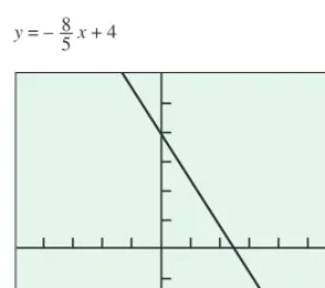
EXAMPLE 5
Analyzing and Graphing a General Linear Equation
Find the slope and y-intercept of the line 8x
5y
20. Graph the line.
SOLUTION
Solve the equation for y
to put the equation in slope-intercept form:
8x
5y
20
5y
8x
20
y
8
5
x
4
This form reveals the slope (m
8
5) and y-intercept (b
4), and puts the equation
in a form suitable for graphing (Figure 1.6).
Now try Exercise 27.
EXAMPLE 6
Writing Equations for Lines
Write an equation for the line through the point (
1, 2) that is
(a)
parallel, and
(b)
perpendicular to the line L:
y
3x
4.
SOLUTION
The line L,
y
3x
4, has slope 3.
(a)
The line y
3(x
1)
2, or y
3x
5, passes through the point (
1, 2), and
is parallel to L
because it has slope 3.
(b)
The line y
(
1
3)(x
1)
2, or y
(
1
3)x
5
3, passes through the point
(
1, 2), and is perpendicular to L
because it has slope
1
3.
Now try Exercise 31.
EXAMPLE 7
Determining a Function
The following table gives values for the linear function f
(x)
mx
b. Determine m
and b.
[–5, 7] by [–2, 6]
[image:5.684.35.184.75.207.2]y = – 8x + 4 5
Figure 1.6 The line 8x5y20. (Example 5)
x ƒ(x)
1 14
31 4
32 13
3SOLUTION
The graph of f
is a line. From the table we know that the following points are on the
line: (
1, 14
3), (1,
4
3), (2,
13
3).
Using the first two points, the slope m
is
m
4
3
1
(14
3)
(
1)
2
6
3.
So f
(x)
3x
b
. Because f
(
1)
14
3, we have
f
(
1)
3(
1)
b
14
3
3
b
b
5
3.
Section 1.1 Lines 7
Thus,
m
3,
b
5
3, and f
(x)
3x
5
3.
We can use either of the other two points determined by the table to check our work.
Now try Exercise 35.Applications
Many important variables are related by linear equations. For example, the relationship
between Fahrenheit temperature and Celsius temperature is linear, a fact we use to
advan-tage in the next example.
EXAMPLE 8
Temperature Conversion
Find the relationship between Fahrenheit and Celsius temperature. Then find the Celsius
equivalent of 90ºF and the Fahrenheit equivalent of
5ºC.
SOLUTION
Because the relationship between the two temperature scales is linear, it has the form
F
mC
b.
The freezing point of water is F
32º or C
0º, while the boiling point
is F
212º or C
100º. Thus,
32
m
•0
b
and
212
m
•100
b,
so b
32 and m
(212
32)
100
9
5. Therefore,
F
9
5
C
32,
or
C
5
9
F
32
.
These relationships let us find equivalent temperatures. The Celsius equivalent of 90ºF is
C
5
9
90
32
32.2°.
The Fahrenheit equivalent of
5ºC is
F
9
5
5
32
23°.
Now try Exercise 43.It can be difficult to see patterns or trends in lists of paired numbers. For this reason, we
sometimes begin by plotting the pairs (such a plot is called a
scatter plot
) to see whether
the corresponding points lie close to a curve of some kind. If they do, and if we can find an
equation y
f
(x) for the curve, then we have a formula that
1.
summarizes the data with a simple expression, and
2.
lets us predict values of y
for other values of x.
The process of finding a curve to fit data is called
regression analysis
and the curve is
called a
regression curve.
There are many useful types of regression curves—power, exponential, logarithmic,
si-nusoidal, and so on. In the next example, we use the calculator’s linear regression feature
to fit the data in Table 1.1 with a line.
EXAMPLE 9
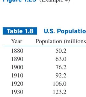
Regression Analysis—–Predicting World Population
Starting with the data in Table 1.1, build a linear model for the growth of the world
pop-ulation. Use the model to predict the world population in the year 2010, and compare
this prediction with the Statistical Abstract prediction of 6812 million.
continued
Some graphing utilities have a feature that enables them to approximate the relationship between variables with a linear equation. We use this feature in Example 9.
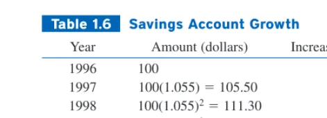
Table 1.1 World Population
Year Population (millions)
1980 4454
1985 4853
1990 5285
1995 5696
2003 6305
2004 6378
2005 6450
SOLUTION
Model
Upon entering the data into the grapher, we find the regression equation to be
ap-proximately
y
79.957x
153848.716,
(1)
where x
represents the year and y
the population in millions.
Figure 1.7a shows the scatter plot for Table 1.1 together with a graph of the regression
line just found. You can see how well the line fits the data.
Why Not Round the Decimals in Equation 1 Even More?
If we do, our final calculation will be way off. Using y80x 153, 849, for instance, gives y6951 when x2010, as compared to y6865, an increase of 86 million. The rule is:
Retain all decimal places while working a problem. Round only at the end.We rounded the coefficients in Equation 1 enough to make it readable, but not enough to hurt the outcome. However, we knew how much we could safely round only from first having done the entire calculation with numbers unrounded.
[1975, 2010] by [4000, 7000]
(a)
Figure 1.7 (Example 9)
Rounding Rule
Round your answer as appropriate, but do not round the numbers in the calcu-lations that lead to it.
Regression Analysis
Regression analysis has four steps:
1.
Plot the data (scatter plot).
2.
Find the regression equation. For a line, it has the form y
mx
b.
3.
Superimpose the graph of the regression equation on the scatter plot to see the fit.
4.
Use the regression equation to predict y-values for particular values of x.
[1975, 2010] by [4000, 7000](b)
X = 2010
Y = 6864.854
Solve Graphically
Our goal is to predict the population in the year 2010. Reading
from the graph in Figure 1.7b, we conclude that when x
is 2010,
y
is approximately
6865.
Confirm Algebraically
Evaluating Equation 1 for x
2010 gives
y
79.957(2010)
153848.716
6865.
Section 1.1 Lines 9
Quick Review 1.1
(For help, go to Section 1.1.)
1. Find the value of ythat corresponds to x3 in y 2 4(x3). 2
2. Find the value of xthat corresponds to y3 in y3 2(x1). 1
In Exercises 3 and 4, find the value of mthat corresponds to the values of xand y.
3. x5, y2, m y x 3 4 1
4. x 1, y 3, m 2 3 y x 54
Section 1.1 Exercises
In Exercises 1–4, find the coordinate increments from Ato B.
1. A(1, 2), B(1,1) 2. A(3, 2), B(1,2)
3. A(3, 1), B(8, 1) 4. A(0, 4), B(0,2) In Exercises 5–8, let Lbe the line determined by points Aand B.
(a) Plot Aand B. (b) Find the slope of L.
(c) Draw the graph of L.
5. A(1,2), B(2, 1) 6. A(2,1), B(1,2)
7. A(2, 3), B(1, 3) 8. A(1, 2), B(1,3) In Exercise 9–12, write an equation for (a)the vertical line and (b)
the horizontal line through the point P.
9. P(3, 2) 10. P(1, 43)
11. P(0,2) 12. P(p, 0)
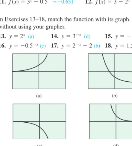
In Exercises 13–16, write the point-slope equation for the line through the point Pwith slope m.
13. P(1, 1), m1 14. P(1, 1), m 1
15. P(0, 3), m2 16. P(4, 0), m 2
In Exercises 17–20, write the slope-intercept equation for the line with slope mand y-intercept b.
17. m3, b 2 18. m 1, b2
19. m 12, b 3 20. m13, b 1 In Exercises 21–24, write a general linear equation for the line through the two points.
21. (0, 0), (2, 3) 22. (1, 1), (2, 1)
23. (2, 0), (2,2) 24. (2, 1), (2,2)
In Exercises 25 and 26, the line contains the origin and the point in the upper right corner of the grapher screen. Write an equation for the line.
25. 26.
In Exercises 27–30, find the (a)slope and (b)y-intercept, and
(c)graph the line.
27. 3x4y12 28. xy2
29. 3 x 4 y
1 30. y2x4
In Exercises 31–34, write an equation for the line through Pthat is
(a)parallel to L, and (b)perpendicular to L.
31. P(0, 0), L:y–x2 32. P(2, 2), L: 2xy4
33. P(2, 4), L:x5 34. P(1, 12), L:y3 In Exercises 35 and 36, a table of values is given for the linear function f(x) mxb.Determine mand b.
35. 36.
x f(x)
2 1
4 4
6 7
x f(x)
1 2
3 9
5 16
[–5, 5] by [–2, 2] [–10, 10] by [–25, 25]
In Exercises 5 and 6, determine whether the ordered pair is a solution to the equation.
5. 3x4y5 6. y 2x5
(a) (2, 14) (b) (3,1) (a) (1, 7) (b) (2, 1)
Yes No Yes No
In Exercises 7 and 8, find the distance between the points.
7. (1, 0), (0, 1) 2 8. (2, 1), (1,13) 5
3
In Exercises 9 and 10, solve for yin terms of x.
9. 4x3y7 10. 2x5y 3
y 4
3x 7
3 y
2 5x
3 5
1. x 2,y 3 2. x2,y 4
x 5,
y0
x0,
y 6
(b)3
(b)0
x3; y2
y x2
y 1
3x1
y3x2
x 1; y 4
3 (a)
3 4 (b)3
m 7
2,
b 3
2
m 3
2,
b 2
(a)–1 (b)2
(a)4
3 (b)4 (a)2 (b)4
x ; y0
x0; y 2
3x– 2y0 y1
3x 4y 2
x 2
(b)Has no slope (undefined) (b)1
3
y 5
2x y
2 5x
13. y1(x– 1) 1 14. y 1(x 1) 1
15. y2(x– 0) 3 16. y 2(x 4) 0 19. y 1
2x 3
31. (a)y x (b)yx 32. (a)y 2x– 2 (b) y 1
2x3 33. (a)x 2 (b)y4 34. (a)y 1
2 (b)x 1
44. Modeling Distance Traveled A car starts from point Pat time t0 and travels at 45 mph.
(a)Write an expression d(t) for the distance the car travels from P.
(b) Graph yd(t).
(c) What is the slope of the graph in (b)? What does it have to do with the car? Slope is 45, which is the speed in miles per hour. (d) Writing to Learn Create a scenario in which tcould have negative values.
(e) Writing to Learn Create a scenario in which the y -inter-cept of yd(t) could be 30.
In Exercises 45 and 46, use linear regression analysis.
45. Table 1.2 shows the mean annual compensation of construction workers.
Table 1.2 Construction Workers’ Average Annual Compensation
Annual Total Compensation
Year (dollars)
1999 42,598
2000 44,764
2001 47,822
2002 48,966
Source:U.S. Bureau of the Census,Statistical Abstract of the United States, 2004–2005.
Table 1.3 Girls’ Ages and Weights
Age (months) Weight (pounds)
19 22
21 23
24 25
27 28
29 31
31 28
34 32
38 34
43 39
In Exercises 37 and 38, find the value of xor yfor which the line through Aand Bhas the given slope m.
37. A(2, 3), B(4,y), m 23 y 1 38. A(8,2), B(x, 2), m2 x 6
39. Revisiting Example 4 Show that you get the same equation in Example 4 if you use the point (3, 4) to write the equation.
40. Writing to Learn x- and y-intercepts
(a) Explain why cand dare the x-intercept and y-intercept, respectively, of the line
x
c d y
1.
(b) How are the x-intercept and y-intercept related to cand din the line
xc dy 2?
41. Parallel and Perpendicular Lines For what value of k are the two lines 2xky3 and xy1 (a)parallel? k2 (b)perpendicular? k 2
Group Activity In Exercises 42–44, work in groups of two or three to solve the problem.
42. Insulation By measuring slopes in the figure below, find the tem-perature change in degrees per inch for the following materials.
(a) gypsum wallboard
(b) fiberglass insulation
(c) wood sheathing
(d) Writing to Learn Which of the materials in (a)–(c) is the best insulator? the poorest? Explain.
0 10°
Distance through wall (inches)
T
emperature (
°
F)
1 2 3 4 5 6 7
0° 20° 30°
40° 50° 60° 70° 80°
Fiberglass between studs Gypsum wallboard
Sheathing
Siding
Air outside at 0°F Air
inside room at 72°F
(a) Find the linear regression equation for the data.
(b) Find the slope of the regression line. What does the slope represent?
(c) Superimpose the graph of the linear regression equation on a scatter plot of the data.
(d) Use the regression equation to predict the construction work-ers’ average annual compensation in the year 2008.about $62,659 46. Table 1.3 lists the ages and weights of nine girls.
43. Pressure under Water The pressure pexperienced by a diver under water is related to the diver’s depth dby an equation of the form pkd1(ka constant). When d0 meters, the pressure is 1 atmosphere. The pressure at 100 meters is 10.94 atmospheres. Find the pressure at 50 meters. 5.97 atmospheres (k0.0994)
(a) Find the linear regression equation for the data.
(b) Find the slope of the regression line. What does the slope represent?
(c) Superimpose the graph of the linear regression equation on a scatter plot of the data.
(d) Use the regression equation to predict the approximate weight of a 30-month-old girl. 29 pounds
d(t) 45t
y 2216.2x 4387470.6
Section 1.1 Lines 11
Standardized Test Questions
You should solve the following problems without using a graphing calculator.
47. True or False The slope of a vertical line is zero. Justify your answer. False. A vertical line has no slope.
48. True or False The slope of a line perpendicular to the line ymxbis 1m. Justify your answer. False. The slope is 1/m. 49. Multiple Choice Which of the following is an equation of the
line through (3, 4) with slope 12? A
(A) y4 1
2(x3) (B) y3
1 2(x4)
(C) y4 2(x3) (D) y4 2(x3)
(E) y32(x4)
50. Multiple Choice Which of the following is an equation of the vertical line through (–2, 4)? E
(A) y4 (B) x2 (C) y 4
(D) x0 (E) x 2
51. Multiple Choice Which of the following is the x-intercept of the line y2x5? D
(A)x 5 (B) x5 (C) x0
(D) x52 (E) x 52
52. Multiple Choice Which of the following is an equation of the line through (2,1) parallel to the line y 3x1? B
(A) y 3x5 (B) y 3x7 (C) y 1 3x
1 3
(D) y 3x1 (E) y 3x4
Extending the Ideas
53. The median price of existing single-family homes has increased con-sistently during the past few years. However, the data in Table 1.4 show that there have been differences in various parts of the country.
54. Fahrenheit versus Celsius We found a relationship between Fahrenheit temperature and Celsius temperature in Example 8.
(a) Is there a temperature at which a Fahrenheit thermometer and a Celsius thermometer give the same reading? If so, what is it?
(b) Writing to Learn Graph y1(95)x32,y2 (59)(x32), and y3xin the same viewing window. Explain how this figure is related to the question in part (a).
55. Parallelogram Three different parallelograms have vertices at (1, 1), (2, 0), and (2, 3). Draw the three and give the coordi-nates of the missing vertices.
56. Parallelogram Show that if the midpoints of consecutive sides of any quadrilateral are connected, the result is a parallelogram.
57. Tangent Line Consider the circle of radius 5 centered at (0, 0). Find an equation of the line tangent to the circle at the point (3, 4).
58. Group ActivityDistance From a Point to a Line This activity investigates how to find the distance from a point P(a,b) to a line L: AxByC.
(a) Write an equation for the line Mthrough Pperpendicular to L.
(b) Find the coordinates of the point Qin which Mand Lintersect.
(c) Find the distance from Pto Q. Distance
Answers
39. y1(x– 3) 4
yx–3 4
yx 1, which is the same equation. 40. (a)When y0,xc; when x0,yd.
(b)The x-intercept is 2cand the y-intercept is 2d.
42. (a)–3.75 degrees/inch (b)–16.1 degrees/inch (c)–7.1 degrees/inch
(d)Best: fiberglass; poorest: gypsum wallboard. The best insulator will have the largest temperature change per inch, because that will allow larger temperature differences on opposite sides of thinner layers. 44. (d)Suppose the car has been traveling 45 mph for several hours when it is
first observed at point Pat time t0.
(e)The car starts at time t0 at a point 30 miles past P. 53. (a)y5980x11,810,220
(b)The rate at which the median price is increasing in dollars per year. (c)y21650x43,105,030
(d)South: $5,980 per year, West: $21,650 per year; more rapidly in the West
56. Suppose that the vertices of the original quadrilateral are (a,b), (c,d), (e,f), and (g,h). When the midpoints are connected, the pairs of opposite
sides of the resulting figure have slopes
e
f
b a
or h
g
d c
, and opposite sides are parallel.
57. y 3
4(x3)4 or y 3 4x
2 4
5
58. (a)y B
A(xa)b
(b)The coordinates are
B2aA2
A C B 2 ABb
,A
2b A2 B C B 2 ABa
AaBbC
A2B
[image:10.684.60.292.493.575.2]2
Table 1.4 Median Price of Single-Family Homes
Year South (dollars) West (dollars)
1999 145,900 173,700
2000 148,000 196,400
2001 155,400 213,600
2002 163,400 238,500
2003 168,100 260,900
Source:U.S. Bureau of the Census,Statistical Abstract of the United States, 2004–2005.
(a) Find the linear regression equation for home cost in the South.
(b) What does the slope of the regression line represent?
(c) Find the linear regression equation for home cost in the West.
(d) Where is the median price increasing more rapidly, in the South or the West?
Functions and Graphs
Functions
The values of one variable often depend on the values for another:
•
The temperature at which water boils depends on elevation (the boiling point drops as
you go up).
•
The amount by which your savings will grow in a year depends on the interest rate
of-fered by the bank.
•
The area of a circle depends on the circle’s radius.
In each of these examples, the value of one variable quantity depends on the value of
another. For example, the boiling temperature of water,
b, depends on the elevation,
e; the
amount of interest,
I, depends on the interest rate,
r.
We call b
and I
dependent variables
because they are determined by the values of the variables e
and r
on which they depend.
The variables e
and r
are
independent variables.
A rule that assigns to each element in one set a unique element in another set is called a
function.
The sets may be sets of any kind and do not have to be the same. A function is
like a machine that assigns a unique output to every allowable input. The inputs make up
the
domain
of the function; the outputs make up the
range
(Figure 1.8).
1.2
What you’ll learn about
• Functions
• Domains and Ranges
• Viewing and Interpreting Graphs
• Even Functions and Odd
Functions——Symmetry
• Functions Defined in Pieces
• Absolute Value Function
• Composite Functions
. . . and why
Functions and graphs form the
basis for understanding
mathe-matics and applications.
x
Input (Domain)
f
Output (Range)
f(x)
Figure 1.8 A “machine” diagram for a function.
In this definition,
D
is the domain of the function and R
is a set containing
the range
(Figure 1.9).
R range set
D domain set (a)
Figure 1.9 (a) A function from a set Dto a set R. (b)Nota function. The assignment is not unique.
R D
(b)
Euler invented a symbolic way to say “y
is a function of x”:
y
f
(x),
which we read as “y
equals f
of x.” This notation enables us to give different functions
dif-ferent names by changing the letters we use. To say that the boiling point of water is a
function of elevation, we can write b
f
(e). To say that the area of a circle is a function of
the circle’s radius, we can write A
A(r), giving the function the same name as the
de-pendent variable.
Leonhard Euler
(1707—1783)
[image:11.684.228.547.476.541.2]Leonhard Euler, the dominant mathematical figure of his century and the most prolific mathematician ever, was also an as-tronomer, physicist, botanist, and chemist, and an expert in oriental languages. His work was the first to give the function concept the prominence that it has in mathematics today. Euler’s collected books and papers fill 72 volumes. This does not count his enormous correspon-dence to approximately 300 addresses. His introductory algebra text, written originally in German (Euler was Swiss), is still available in English translation.
DEFINITION
Function
Section 1.2 Functions and Graphs 13
The notation y
f
(x) gives a way to denote specific values of a function. The value of f
at a
can be written as f
(a), read “f
of a.”
EXAMPLE 1
The Circle-Area Function
Write a formula that expresses the area of a circle as a function of its radius. Use the
formula to find the area of a circle of radius 2 in.
SOLUTION
If the radius of the circle is r, then the area A(r) of the circle can be expressed as
A(r)
p
r
2. The area of a circle of radius 2 can be found by evaluating the function A(r)
at r
2.
A(2)
p
(2)
24
p
The area of a circle of radius 2 is 4
p
in
2.
Now try Exercise 3.Domains and Ranges
In Example 1, the domain of the function is restricted by context: the independent variable
is a radius and must be positive. When we define a function y
f
(x) with a formula and
the domain is not stated explicitly or restricted by context, the domain is assumed to be the
largest set of x-values for which the formula gives real y-values—the so-called
natural
domain.
If we want to restrict the domain, we must say so. The domain of y
x
2is
under-stood to be the entire set of real numbers. We must write “y
x
2,
x
0” if we want to
re-strict the function to positive values of x.
The domains and ranges of many real-valued functions of a real variable are intervals or
combinations of intervals. The intervals may be open, closed, or half-open (Figures 1.10 and
1.11) and finite or infinite (Figure 1.12).
x a
Notation: a ≤ ≤x bor [a, b] Name: Closed interval ab b
x a
Notation: a < x < b or (a, b) Name: Open interval ab
b
Figure 1.10 Open and closed finite intervals.
Notation: a x < b or [a, b)
x a
Notation: a < x b
≤
≤ or (a, b] Open at a and closed at b
b x a
Closed at a and open at b b
Figure 1.11 Half-open finite intervals.
The endpoints of an interval make up the interval’s
boundary
and are called
boundary points.
The remaining points make up the interval’s
interior
and are called
interior points. Closed intervals
contain their boundary points.
Open intervals
con-tain no boundary points. Every point of an open interval is an interior point of the
interval.
Viewing and Interpreting Graphs
The points (x,
y) in the plane whose coordinates are the input-output pairs of a function
y
ƒ(x) make up the function’s
graph.
The graph of the function y
x
2, for example,
is the set of points with coordinates (x,
y) for which y
equals x
2.
xb or (– , b] Notation:
x b or (–, b) Notation:
ax or [a, ) Notation:
a x or (a, ) Notation:
– x
Notation:
0
a
a
b
b
or (–, )
≤
≤
The set of all real numbers Name:
The set of numbers greater than a
Name:
The set of numbers greater than or equal to a
Name:
The set of numbers less than b
Name:
The set of numbers less than or equal to b
Name:
Figure 1.12 Infinite intervals—rays on the number line and the number line itself. The symbol (infinity) is used merely for convenience; it does not mean there is a number .
EXAMPLE 2
Identifying Domain and Range of a Function
Identify the domain and range, and then sketch a graph of the function.
(a)
y
1
x
(b)
y
x
SOLUTION
(a)
The formula gives a real y-value for every real x-value except x
0. (We cannot divide
any number by 0.) The domain is (
, 0)
(0,
). The value y
takes on every real
num-ber except y
0. (y
c
0 if x
1
c) The range is also (
, 0)
(0,
). A sketch is
shown in Figure 1.13a.
x y
1 2 3 4
–4
–1
(a) –1
–2 –2
–4 –3 –3
2 3 4
1
Figure 1.13 A sketch of the graph of (a) y 1xand (b)
y
x
. (Example 2)(b)
The formula gives a real number only when x
is positive or zero. The domain is
[0,
). Because
x
denotes the principal square root of x,
y
is greater than or equal to
zero. The range is also [0,
). A sketch is shown in Figure 1.13b.
Now try Exercise 9.
Graphing with pencil and paper requires that you develop graph drawing
skills. Graphing
with a grapher (graphing calculator) requires that you develop graph viewing
skills.
Graph Viewing Skills
1.
Recognize that the graph is reasonable.
2.
See all the important characteristics of the graph.
3.
Interpret those characteristics.
4.
Recognize grapher failure.
Being able to recognize that a graph is reasonable comes with experience. You need to
know the basic functions, their graphs, and how changes in their equations affect the
graphs.
Grapher failure
occurs when the graph produced by a grapher is less than precise—or
even incorrect—usually due to the limitations of the screen resolution of the grapher.
x y
1 2 3 4 5 6
–1
(b) –1
–2 –2
2 3 4
Section 1.2 Functions and Graphs 15
Graphing y= x2/3—–Possible Grapher Failure
On some graphing calculators you need to enter this function as y(x2)1/3or
y(x1/3)2to obtain a correct graph. Try graphing this function on your gra-pher.
EXAMPLE 3
Identifying Domain and Range of a Function
Use a grapher to identify the domain and range, and then draw a graph of the function.
(a)
y
4
x
2(b)
y
x
2/3SOLUTION
(a)
Figure 1.14a shows a graph of the function for
4.7
x
4.7 and
3.1
y
3.1, that is, the viewing window [
4.7, 4.7] by [
3.1, 3.1], with
x-scale
y-scale
1. The graph appears to be the upper half of a circle. The
do-main appears to be [
2, 2]. This observation is correct because we must have
4
x
20, or equivalently,
2
x
2. The range appears to be [0, 2], which can
also be verified algebraically.
(b)
Figure 1.14b shows a graph of the function in the viewing window
[
4.7, 4.7] by [
2, 4], with
x-scale
y-scale
1. The domain appears to be
(
,
), which we can verify by observing that x
2/3(
3
x
)
2. Also the range is
[0,
) by the same observation.
Now try Exercise 15.Even Functions and Odd Functions—Symmetry
The graphs of even
and odd
functions have important symmetry properties.
[–4.7, 4.7] by [–3.1, 3.1] (a)
y = 4 – x2
[–4.7, 4.7] by [–2, 4]
(b)
y = x2 / 3
Figure 1.14 The graph of (a)
y
4
x
2and (b)y
x
2/3. (Example 3)x y
O y x3
(x, y)
(b) (–x, –y)
Figure 1.15 (a) The graph of yx2
(an even function) is symmetric about the y-axis. (b) The graph of yx3(an odd
function) is symmetric about the origin.
The names even and odd come from powers of x.
If y
is an even power of x, as in y
x
2or
y
x
4, it is an even function of x
(because (
x)
2x
2and (
x)
4x
4). If y
is an odd power
of x, as in y
x
or y
x
3, it is an odd function of x
(because (
x)
1x
and (
x)
3x
3).
The graph of an even function is
symmetric about the
y
-axis.
Since f
(
x)
f
(x), a point
(x,
y) lies on the graph if and only if the point (
x,
y) lies on the graph (Figure 1.15a).
The graph of an odd function is
symmetric about the origin.
Since f
(
x) =
f
(x), a
point (x,
y) lies on the graph if and only if the point (
x,
y) lies on the graph (Figure 1.15b).
xO
y x2
(x, y)
(a) (–x, y)
y
DEFINITIONS
Even Function, Odd Function
A function y
ƒ(x) is an
even function of
x
if f
x
f
x
,
odd function of
x
if f
x
f
x
,
for every x
in the function’s domain.
Equivalently, a graph is symmetric about the origin if a rotation of 180º about the origin
leaves the graph unchanged.
EXAMPLE 4
Recognizing Even and Odd Functions
f
(x)
x
2Even function: (
x)
2x
2for all x; symmetry about y-axis.
f
(x)
x
21
Even function: (
x)
21
x
21 for all x; symmetry about
y-axis (Figure 1.16a).
f
(x)
x
Odd function: (
x)
x
for all x; symmetry about the origin.
f
(x)
x
1 Not
odd:
f
(
x)
x
1, but
f
(x)
x
1. The two are not
equal.
Not even: (
x)
1
x
1 for all x
0 (Figure 1.16b).
Now try Exercises 21 and 23.
It is useful in graphing to recognize even and odd functions. Once we know the graph
of either type of function on one side of the y-axis, we know its graph on both sides.
Functions Defined in Pieces
While some functions are defined by single formulas, others are defined by applying
different formulas to different parts of their domains.
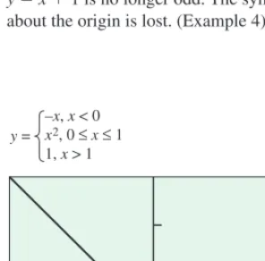
EXAMPLE 5
Graphing Piecewise-Defined Functions
x,
x
0
Graph y
f
x
{
x
2,
0
x
1
1,
x
1.
SOLUTION
The values of f
are given by three separate formulas:
y
x
when x
0,
y
x
2when
0
x
1, and y
1 when x
1. However, the function is just one function,
whose
domain is the entire set of real numbers (Figure 1.17).
Now try Exercise 33.EXAMPLE 6
Writing Formulas for Piecewise Functions
Write a formula for the function y
f
(x) whose graph consists of the two line
segments in Figure 1.18.
SOLUTION
We find formulas for the segments from (0, 0) to (1, 1) and from (1, 0) to (2, 1) and
piece them together in the manner of Example 5.
Segment from (0, 0) to (1, 1)
The line through (0, 0) and (1, 1) has slope
m
(1
0)
(1
0)
1 and y-intercept b
0. Its slope-intercept equation is y
x.
The segment from (0, 0) to (1, 1) that includes the point (0, 0) but not the point (1, 1) is
the graph of the function y
x
restricted to the half-open interval 0
x
1, namely,
y
x,
0
x
1.
xy
0 1
yx2 1
yx2
(a)
x y
0 1
–1
yx 1
yx
[image:15.684.47.179.57.386.2](b)
Figure 1.16 (a) When we add the con-stant term 1 to the function yx2, the
resulting function yx21 is still even
and its graph is still symmetric about the y -axis. (b) When we add the constant term 1 to the function yx, the resulting function yx1 is no longer odd. The symmetry about the origin is lost. (Example 4)
[–3, 3] by [–1, 3]
y =
–x, x < 0
x2, 0 ≤x≤ 1
1, x > 1
Figure 1.17 The graph of a piecewise
[image:15.684.36.184.517.663.2]Section 1.2 Functions and Graphs 17
Segment from (1, 0) to (2, 1)
The line through (1, 0) and (2, 1) has slope
m
(1
0)
(2
1)
1 and passes through the point (1, 0). The corresponding
point-slope equation for the line is
y
1
x
1
0,
or
y
x
1.
The segment from (1, 0) to (2, 1) that includes both endpoints is the graph of y
x
1
restricted to the closed interval 1
x
2, namely,
y
x
1,
1
x
2.
Piecewise Formula
Combining the formulas for the two pieces of the graph,
we obtain
x,
0
x
1
f
x
{x
1,
1
x
2.
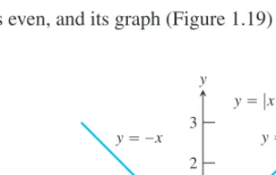
Now try Exercise 43.Absolute Value Function
The
absolute value function
y
x
is defined piecewise by the formula
x,
x
0
x
{x,
x
0.
The function is even, and its graph (Figure 1.19) is symmetric about the y-axis.
xy
1 1
y f(x)
0 2
(1, 1) (2, 1)
Figure 1.18 The segment on the left con-tains (0, 0) but not (1, 1). The segment on the right contains both of its endpoints. (Example 6)
x y
0 1 1 3
2
2 3 –1
– 2 – 3
y x y – x
[image:16.684.322.474.349.445.2]yx
Figure 1.19 The absolute value function has domain ,and range 0,.
[–4, 8] by [–3, 5]
y = |x– 2| – 1
Figure 1.20 The lowest point of the graph of fxx21 is 2,1. (Example 7)
x
g g(x) f f(g(x))
Figure 1.21 Two functions can be com-posed when a portion of the range of the first lies in the domain of the second.
EXAMPLE 7
Using Transformations
Draw the graph of f
x
x
2
1. Then find the domain and range.
SOLUTION
The graph of f
is the graph of the absolute value function shifted 2 units horizontally to
the right and 1 unit vertically downward (Figure 1.20). The domain of ƒ
is
,
and
the range is
1,
.
Now try Exercise 49.Composite Functions
“f
of g
of x”) is the
composite of
g
and
f.
It is made by composing g
and ƒ
in the order of
first g, then f.
The usual “stand-alone” notation for this composite is f
g, which is read as
“f
of g.” Thus, the value of f
g
at x
is
f
g
(x)
f
(g(x)).
EXAMPLE 8
Composing Functions
Find a formula for f
(g(x)) if g(x)
x
2and f
(x)
x
7. Then find f
(g(2)).
SOLUTION
To find f
(g(x)), we replace x
in the formula f
(x)
x
7 by the expression given for
g(x).
f
x
x
7
f
g
x
g
x
7
x
27
We then find the value of f
(g(2)) by substituting 2 for x.
f
g
2
2
27
3
Now try Exercise 51
.
Composing Functions
Some graphers allow a function such as y
1to be used as the independent variable of
another function. With such a grapher, we can compose functions.
1.
Enter the functions y
1f
(x)
4
x
2,
y
2
g(x)
x
,
y
3y
2(y
1(x)), and
y
4y
1(y
2(x)). Which of y
3and y
4corresponds to f
g? to g
f
?
2.
Graph y
1,
y
2, and y
3and make conjectures about the domain and range of y
3.
3.
Graph y
1,
y
2, and y
4and make conjectures about the domain and range of y
4.
4.
Confirm your conjectures algebraically by finding formulas for y
3and y
4.
EXPLORATION 1
Quick Review 1.2
(For help, go to Appendix A1 and Section 1.2.)
In Exercises 1–6, solve for x.
1. 3x15x3 [2,) 2. x(x2) 0
3. x34 [1, 7] 4. x25
5. x216 (4, 4) 6. 9x20 [3, 3]
In Exercises 7 and 8, describe how the graph of ƒcan be transformed to the graph of g.
7. f(x)x2, g(x) (x2)23 8. fxx, gxx52
In Exercises 9–12, find all real solutions to the equations.
9. f(x) x25
(a) ƒ(x) 4 (b) f(x) 6
10. f(x) 1x
(a) fx 5 (b) f(x) 0
11. fxx7
(a) f(x) 4 (b) f(x) 1
12. fx3x1
(a) f(x) 2 (b) f(x) 3
(, 0) (2,)
(,3] [7,)
7. Translate the graph of f 2 units left and 3 units downward. 8. Translate the graph of f 5 units right and 2 units upward.
x 3, 3 No real solution
x 7 x28
x9 x 6
(a)x 1