Competing Conventions
∗
Philip R. Neary
†April 30, 2012
Abstract
This paper introduces a new coordination problem for a large but finite popu-lation - The Language Game. The population is partitioned into two groups of identical agents. Each player shares a common two-action strategy set and in-teracts pairwise with everyone else. Both symmetric profiles are Pareto-efficient strict equilibria, but the groups rank them differently. The profile where success-ful coordination occurs only within-group, with each group adopting their most preferred equilibrium action, is also an equilibrium provided the smaller group’s preferences are sufficiently strong. In all dynamically stable long-run outcomes, players in the same group adopt the same action. Three properties, that do not matter for equilibrium selection in standard homogeneous agent models, do matter in the Language Game. These are: group size, strength of group prefer-ences, and rates of group adaptiveness (“group dynamism”). A relative increase in group size and group dynamism is always weakly beneficial.
∗I would like to thank Sarada, Nageeb Ali, Prashant Bharadwaj, Larry Blume, Tiffany Chou, Vince Crawford, Silke Januszewski Forbes, Dan Friedman, Dalia Ghanem, Roger Gordon, Youjin Hahn, Oana Hirakawa, Matt Jackson, Michihiro Kandori, Chulyoung Kim, David Levine, Daniel Lima, Stephen Morris, Peter Neary, Paul Niehaus, Frances Ruane, Bill Sandholm, Lucas Siga, James Slevin, Bernhard von Stengel, John Sutton, Joel Watson, Hee-Seung Yang, Peyton Young, and seminar participants at UCSD, University of Colorado Boulder, The Brattle Group, LSE, and Royal Holloway for helpful comments. Two anonymous referees and an associate editor made many good suggestions that improved the paper considerably. I would especially like to thank Joel Sobel for all his help. Remaining errors are mine.
“Nobody will ever win the battle of the sexes.
There’s just too much fraternizing with the enemy.”
- Henry Kissinger
1
Introduction
A large population coordination problem is one wherein all parties can realize mutual
gains, but only by making mutually consistent decisions. Often, such mutually
consis-tent decisions require that everybody behave identically, but on occasion they do not.
For example, while writing academic papers in English is a must since English is the
language of science, and driving on the opposite side of the road as the oncoming traffic
hardly seems wise, it may still make sense to buy a Mac even if it is only your friends
who use them.
The emergence of coordinated outcomes in large societies, often referred to as
con-ventions (Lewis, 1969; Young, 1993, 1996, 2001), is conventionally modelled using the framework of evolutionary game theory. In the simplest model, due toKandori, Mailath, and Rob (1993) (hereafter KMR), a large population of homogeneous players are ran-domly matched to play a symmetriclocal-interaction 2×2 game of pure coordination.
This situation is then repeated indefinitely with players assumed to be myopic
best-responders. Coordination is guaranteed in the long run, the only question is which
strict equilibrium (convention) the population will coordinate on.1 However, by
con-struction, KMR’s model can only be used for studying the emergence of conventions in
societies where all agents have identical preferences. Furthermore, since everyone is the
same, all players long for the same coordinated outcome, and so the only level at which
competition occurs is at that of the strategy. This is limiting, since in many situations
of interest people have different tastes, and so what might be best for some may not be
best for all.
In this paper, I introduce “The Language Game”, that allows the study of
conven-tions in a particular heterogeneous environment.2 The population is composed of not
one, but two homogeneous groups with differing preferences.3 Each player has the same
1Young(1993) describes a broad class of games for which such “lock in” will certainly occur. 2A similar model is presented in Quilter(2007).
3Another setting with two homogeneous groups with (potentially) differing preferences are the
two-action strategy set and interacts pairwise with everyone else. Utilities are the sum
of payoffs earned from playing the field, where the same action must be used with each
opponent. Uniform adoption of either action is always a strict equilibrium, but the
groups rank them differently. If the smaller group has sufficiently strong preferences,
then the members of each group adopting their preferred action, and thus forfeiting
coordination with those of the other group, can also be supported in equilibrium.
Next, the Language Game becomes the stage game of a repeated interaction. Time
is discrete, begins at t = 0, and goes forever. Payoffs are received every period and actions for tomorrow must be chosen at the end of today. The same assumptions on
individual behaviour used in KMR generate population dynamics that will lock in on
some convention with probability one. I then turn to the issue ofequilibrium selection,
employing the concept of stochastic stability, introduced in the seminal work of
(Fos-ter and Young, 1990). The basic idea is that players occasionally, and independently, choose non-optimal responses. Such “mutations” perturb the dynamics, enabling crisp
predictions to be made about long-run behaviour. Equilibrium selection in the
Lan-guage Game depends on three factors that have no bearing in KMR’s model. They
are: group size, group payoffs, and group dynamism (how regularly members of a given
group react).4 These properties can be traded off against each other. Increased group
dynamism and greater group numbers are always desirable. However, perhaps
surpris-ingly, stronger preferences need not be.
Welfare issues are interesting. In the homogeneous agent model, for any convention
each player’s behaviour and payoff are identical. As such, the literature has focused
primarily on the tension that arises when the “good” Pareto-dominant equilibrium
action does not coincide with the “safe” risk-dominant one. Foster and Young (1990), KMR and Young (1993) were the first to show that evolutionary forces coupled with mutations will propel population behaviour towards risk-dominance.5 Only
Pareto-players are matched against a population of “column” Pareto-players to play an asymmetric game, e.g. Battle of the Sexes. However, and this is a big difference, it is still the case that players from each group only interact with one other type of player (those from the other group). Thus, despite adding heterogeneity, there is still only one common local interaction.
4“Group dynamism” permits many interpretations. It can be thought of as how sensitive, on
average, a particular group’s members are to their surroundings; as differences in inertia - life in the city is more hectic than life in the countryside; as the frequency of death and replacement; as adjustment costs varying across group since some find change less burdensome; or even as variable information access which would enable greater transparency in decision making.
Pareto-efficient equilibria are selected in the Language Game.
The “Language Game” moniker is due to the model’s applicability to issues of
compatibility: successful coordination is good, while all types of failed coordination
are equally bad. An example is the adoption of technological standards (Katz and
Shapiro, 1985; Farrell and Saloner, 1985; Arthur, 1989). The key observation in this literature is one of network effects, whereby the usefulness of a technology is increasing
in the number of its users. The homogeneity of existing models means the population
collectively agrees on the optimal standard, and whatever standard does emerge is
adopted by one and all. The Language Game helps to organize observations because
often subsets of the population have inherent preferences for different standards, and
often multiple standards coexist. Section 2illustrates this with an example.
It has been traditional in evolutionary models to view the players as being drawn
from a single population. This assumption constrains all local interactions to be the
same and limits the scope of the analysis. The main contribution of this paper is
to provide an uncomplicated model, with immediate economic applications, with this
assumption relaxed. However, while the Language Game is the first detailed setting
with multiple populations interacting together, what I believe to be the major insight
(that of multiple populations all interacting together) is not as novel as I’d hoped, and I
would be remiss not to mention some other work.6 Friedman(1998) discusses a general
setting with two populations where, in addition to asymmetric interactions, there are
also “own-population effects”. Cressman, Garay, and Hofbauer (2001) characterize
Evolutionary Stable Strategies (Smith and Price, 1973) for what they call N-Species Frequency-Dependent Interactions; the textbookCressman (2003) explores these ideas further. Quilter (2007) analyses a similar model, but focuses on how the specifics of the perturbations can affect selection.7
The plan of the paper is as follows. In the next section, I present a simple example
dominant equilibrium action can emerge in similar settings. Ely(2002),Oechssler(1999) andOechssler
(1997) are models with endogenous local interactions, Canals and Vega-Redondo (1998) and Robson and Vega-Redondo(1996) vary the frequency with which players may interact, while Kim and Sobel
(1995) add a round of costless communication, “cheap talk”, before actions are taken.
6Thanks to David Levine, Bill Sandholm, and an anonymous referee for drawing my attention to
these papers.
7Other papers with heterogeneity include Carvalho(2010), where ‘taboos’ are imposed on certain
that demonstrates how homogeneous groups with heterogeneous preferences can be
a more natural way to think about certain large population situations, in particular
technology adoption. The Language Game is formally defined in Section 3, where I
also characterize the set of pure strategy equilibria. Section 4 shows how decisions
at the individual level are aggregated to yield group dynamics, and illustrates via an
example how path dependence may be influenced by the details of the dynamics. This
analysis is carried forward to Section5 which contains the main results on equilibrium
selection. Section 6 looks at welfare properties of selected equilibria, while Section 7
examines how the set of selected equilibria varies as Language Game parameters change.
Section8 concludes and discusses some potential avenues for future work.
2
A Story
The story is an extension of one from KMR. I begin by reminding the reader of theirs
and then build on it.
There is a university dormitory of 10 identical students, referred to as GroupA. Each Group A student chooses a computer system from the set {a, b}. Each evening, the students assemble in the study hall, where everybody encounters everyone else. When
two students interact, they can collaborate by playing games, sharing files, swapping
add-ons, etc. But - and this is key - meetings are fruitful if and only if both students use
the same system. Assuming that system a is inherently superior to system b induces the following local-interaction pure coordination game,GAA,
AI
AII
a b a 3,3 0,0
b 0,0 2,2
whereAI andAII are any pair of GroupA students. The local interactionGAA has two
Following KMR, assume that students occasionally have the opportunity to change
their computer, and that students are myopic in that decisions taken are best-responses
to the current distribution of computers. This generates Darwinian dynamics. Initial
conditions are key: if more than two fifths of the population begins using system a
(5 or more since the population is of size 10), then outcome a will be reached; while
if 6 or more students start out using b, then b will be the final resting point. The reasoning is simple, all players collectively agree on what action is a best-response, so
the best-response today must be at least as good a response tomorrow as the number
of players taking that action can only (weakly) increase. Thus population behaviour is
always drifting towards either aor b.
However, when noise in the form of individual trembles/mistakes/experimentation
is incorporated into the dynamics, it is possible to select between strict equilibrium
outcomes. Suppose that the probability that a student mistakenly chooses the computer
that is not an optimal response is given byε. It takes 5 or more simultaneously occurring mistakes to dislodge the system from b, and 6 or more to get away from a. The most
likely events of this form occur with probability of orders ε5 and ε6 respectively. For small values of ε, ε6 ε5, and so KMR conclude that when agents are myopic best-responders, who occasionally make mistakes, that outcome a is far more likely to be
observed in the long run. Equilibriuma is said to be selected.
A key component of the above story was systema’sinherent superiority to systemb. While in many coordination problems it is plausible to believe that coordination on one
particular strategy is better (by any metric) than another, words like “better” derive
from primitive preferences, and preferences are individual by nature. In a population
with heterogeneous agents, what might be best for some may not be best for all.
To illustrate the impact of adding heterogeneity, consider the following extension to
the above story. Suppose Group A are “slackers” - they must also do coursework on their machines, but their main use for computers is playing games. Instead of assuming
that computer system a is flat out better than b, suppose that system a more readily supports gaming platforms, which justifies GroupA’s preference for coordinating on it. Suppose further that there is another dorm of 5 more students, referred to as Group
B, in the next building. Every evening, these 5 Group B students meet in a separate study hall and exchange software, etc. Again, interactions are beneficial if and only if
“serious” scholars, and that platform b suits these needs better. The local interaction between two GroupB students is thus given by the following pure coordination game,
GBB,
BI
BII
a b a 1,1 0,0
b 0,0 2,2
whereBIand BII are any two GroupB students. By an analysis identical to that given
above for GroupA, left to their own devices GroupB will adopt computer system b in the long run.8 Now, consider the 15 person population as a whole. Writing a
group-symmetric profile9 as a 2-dimensional vector, with the Group A profile written first,
there are 4 strict equilibria: (a,a),(a,b),(b,a),(b,b). The selected equilibrium is (a,b).
Now suppose that in an effort to free up space, the university stipulates that both
groups should study Group A’s larger study room which can accommodate 5 extra bodies (this frees up the smaller study room for other activities). So now, all 15 students
meet in the same room every evening. Everybody interacts with everybody else, and
within-group local interactions are as before. It remains to specify the local interaction
occurring between students from opposite groups. This is described by the following
coordination game,GAB, in which the row player,Ai, is from GroupA, and the column
player, Bj, is from GroupB,
Ai
Bj
a b a 3,1 0,0
b 0,0 2,2
The local interaction GAB is not symmetric. It has two Pareto-efficient pure
strat-egy equilibria, (a, a) and (b, b), over which players’ preferences disagree. Considering the population coordination problem, interactions are now occurring both within- and
8The probability of Group B transitioning from ato boccurs with probability of order ε2, while
that of transitioning frombtoa occurs with probability of orderε4.
9A group-symmetric profile is one in which those in the same group take the same action. A
across-group. Each Group A student interacts with 9 fellow Group A students and 5 GroupBstudents, while each GroupB student interacts with 4 other GroupBstudents and 10 Group A students. The only group-symmetric equilibria to this new situation are (a,a) and (b,b).10 While both are Pareto-efficient, the 10 GroupA students prefer (a,a), while the 5 Group B students view (b,b) as most desirable.
I now pause and ask the reader to predict what they think the selected outcome
will be (recalling that (a,a) and (b,b) are the only viable candidates). One conjecture might be the following. Even though behaviour evolves in a decentralised manner via
individual best-responses, the greater Group A numbers should somehow collectively force its preferred outcome, (a,a), onto the population at large. However, this goes against the equally simple theory that (relative) strength of preferences should be the
determining factor. If preferences were the key ingredient, the selection prediction in
this example would be tilted towards Group B’s preferred outcome, (b,b).
Clearly group sizes and group preferences are important. However, it turns out that
selection also depends on a variety of additional factors aside from these. The first of
these is noise (individual mistakes). In the original story with only GroupA, all agents were identical so assuming they all make time- and profile-independent mistakes with
equal probability seemed not completely unreasonable. However, with a population
composed of two “types” of agents, if Group A students tremble with probability εA
while Group B students tremble with probability εB, there is no obvious reason to
conclude that εA=εB.
The second complicating factor is a property I refer to as group dynamism. Group
dynamism can be thought of as the rate at which a group responds. It may be that
GroupAstudents are more lethargic than Group B students. Perhaps on average only one GroupAstudent updates his action in a given period, whereas all GroupBstudents update their action every period. In the real world, there is no reason to suppose that
different groups respond at identical rates.
However, with these caveats in mind, let’s begin by assuming that: (1) payoffs are
as given in GAA, GAB and GBB; (2) the group sizes are 10 and 5 for Groups A and
B respectively; (3) mistakes are such that εA = εB = ε; and (4) both groups evolve
according to the best-reply dynamic in which all students react every period.
10While (a,b), and (b,a) were equilibria when the two groups were unconnected, they are no longer
Suppose first that the population profile is (b,b). Any Group B student needs to see a minimum of 10 others taking action a in order to switch his/her action, while a Group A student needs to see a minimum of 7. Let’s say between 7 and 9 students accidentally chose actiona(it is not important how these students are distributed across the two groups). In the following period, all GroupB students choose action b, but all Group A students choose action a, so that the new profile is (a,b). With no further mistakes, all students take action a the following period. The conclusion is that 7 or more simultaneous mistakes are sufficient to shift the population from (b,b) to (a,a). Now assume that the current profile is (a,a). If between 6 and 8 mistakes occur whereby students accidentally choose action b, it is enough to induce the 5 Group B
students to take actionb, but not enough to induce the 10 Group Astudents to do so. Thus, next period’s profile is (a,b), and with no further mistakes, the system reverts to (a,a). It can be computed that a minimum of 9 simultaneous mistakes are required to shift the system from (b,b) to (a,a).
Transitioning from (a,a) to (b,b) requires an event that occurs with probability of order ε9, while transitioning from (b,b) to (a,a) one with probability of order ε7. For small values of ε, the second transition is far more likely. So provided that: (i) everybody interacts with everybody else; (ii) both groups respond according to best-reply dynamics; (iii) the probability of a student making a mistake is small, equal for all students, and independent of the current population profile; and (iv) payoffs and group-sizes are as specified above. Thus, the informal analysis above concludes that
the selected equilibrium will be (a,a).
Now suppose that the groups adapt at different rates. The situation is as before
except for the dynamics. Now, every period, three Group B students best-respond, while only one Group A student best-responds. Again let us calculate how easy it is to dislodge the population from each of the equilibria. The bounds on player numbers
from before are derived from preferences and group sizes, not dynamics, so those have
not changed. The difference in this analysis is that it will matter exactly who is
mak-ing mistakes. For a pictorial explanation of why it matters who makes mistakes, the
interested reader should look ahead to Figures1 and 2in Section 4.2.
actiona, so that the total number taking action a is increased to 8. The following pe-riod 8 GroupA students are using action a. And so on. Once all 10 Group Astudents are taking action a, action a becomes optimal for Group B students. After two more periods, all of Group B adopts it. Thus, 7 of the “right kind” of mistakes are enough to transition from (b,b) to (a,a).
Now let the current profile be (a,a), and suppose that 6 GroupA students acciden-tally choose action b (again, it matters that these 6 students are from Group A). At this new profile, Group preferences disagree. The following period, 3 GroupB students adopt action b, while one of the 6 Group A students who mistakenly chose action b
reverts to action a. Thus, there are 8 = 3 + (6−1) students taking action b. Next period, all GroupB students adopt actionb while 4 GroupA players do, and so there are now 9 = 5 + (5−1) students taking action b. This is enough for all for Group
A students to prefer action b. From this new situation, by an analysis similar to the previous paragraph, population behaviour moves incrementally to (b,b).
Under these different dynamics, transitioning from (b,b) to (a,a) still occurs with probability of orderε7. More importantly however, the likelihood of transitioning from (a,a) to (b,b) has been lowered to ε6. So in this case, the analysis concludes that equilibrium (b,b) will be selected.
So what, the reader might ask, is the point of this section? There is certainly no
hint of a crisp result like the risk-dominance predictions of KMR and Young (1993). But in fact, the lack of a clean result is precisely the point. That group size and
strength of payoffs affect long-run behaviour is intuitive but not predicted by KMR’s
homogeneous model. In that framework, once an equilibrium is risk-dominant it is
selected (even though it may be Pareto-dominated to an arbitrary extent), and this is
of course independent of population size.
3
The Language Game
3.1
The Model
The Language Game, G, is defined as the tuple {N,Π, S,G}, where N :={1, . . . , N}
the binary action set common to all players; G := GAA, GAB, GBB is the collection
oflocal interactions, where GAA is the pairwise exchange between a player from Group
A and a player from Group A, etc. The local interactions are given as follows,
GAA GBB
A1
A2
a b
a p, p 0,0
b 0,0 1−p,1−p B1
B2
a b
a 1−q,1−q 0,0
b 0,0 q, q GAB
A
B
a b
a p,1−q 0,0
b 0,0 1−p, q
where p, q ∈ (1/2,1), so that Group A members always prefer to coordinate on a, and GroupB members always prefer to coordinate onb.
The Language Game is a simultaneous move game and players do not randomize.
Utilities are the sum of payoffs earned from playing the field, where the same action
must be used with one and all. Local interactions are opponent-independent in that a
player’s payoff depends only on the actions chosen and not the other player’s identity.
Thus, a player cares only about the number of others who choose the same action, but
not who those others are.
With only two “types” of agent, population behaviour can be written concisely. Let
[ω]Kdenote the number of players in groupK ∈Π using actiona. Callω = [ω]A,[ω]B
thestate of the play, where thestate space is Ω :=0, . . . , NA ×
K ∈Π receives from taking actions ∈ {a, b} in state ω, written UK(s;ω), is given by
UA(a;ω) :=
na−1
p (1)
UA(b;ω) :=N −na−1
(1−p) (2)
UB(a;ω) :=na−1
(1−q) (3)
UB(b;ω) :=N −na−1
q (4)
Before discussing individual behaviour, I will mention genericity. Letting N :=
{1,2, . . .}, the set of Language Games can be parameterized by Θ = {(NA, NB, p, q) :
NA, NB ∈
N\ {1};p, q ∈(1/2,1)}. For a given gameG ∈Θ and a given group K ∈Π,
the statement “if there does not exist a state ω ∈ Ω such that UK(a;ω) = UK(b;ω)”,
will be abbreviated to “genK”. If there exists such a state, the shorthand is “ngenK”.
The subset of the parameter space for which any indifference occurs can be shown to
have a closure of measure zero specifically, for a givenNA,NB, andp, there is only one value ofq such that UB(a;ω) = UB(b;ω)
and so when both genA and genB, following
standard terminology I sayG is generic. Otherwise,G isnongeneric.
3.2
Individual Behaviour
Let R denote the real line, and R+ its positive part. For any x ∈ R, let dxe :=
min{n∈N|x≤n} and bxc:= max{n ∈N|x≥n}. Define the following,11
nAa := minna
UA(a;ω)> UA(b;ω) =d(1−p)N + (2p−1)e, (5)
nBa := minna
UB(a;ω)> UB(b;ω) =dq(N −2) + 1e, (6)
nAb := minnb
UA(a;ω)< UA(b;ω) =dp(N −2) + 1e, (7)
nBb := minnb
UB(a;ω)< UB(b;ω) =d(1−q)N + (2q−1)e (8)
nA
a is the number of players currently taking action a for a player from Group A to
strictly prefer action a, etc. When p = q, by symmetry nA
a = nBb and nAb = nBa. This
appears to suggest that the strategic situation is mirrored for groups A and B. While this is true at the individual level, it need not be true at the level of the group.
Let ΩA,ab and ΩB,ab denote the set of states such that A players and B players respectively strictly prefer action a to actionb. Similarly for ΩA,ba and ΩB,ba. Thus we can write
ΩA,ab :=nω ∈Ω [ω]A+ [ω]B ≥nAa o
(9)
ΩB,ab :=nω ∈Ω [ω]A+ [ω]B ≥nBa o
(10)
ΩA,ba:=nω ∈Ω [ω]A+ [ω]B ≤N −nAb o
(11)
ΩB,ba:=
n
ω ∈Ω [ω]A+ [ω]B ≤N −nBb o
(12)
Sets ΩA,ab, ΩB,ab, ΩA,ba, and ΩB,ba are defined likewise but for weak preference.
Generically, these sets of weak- and strict-preference coincide. Letting ⊆ (⊂) denote
weak (strict) inclusion, we have the following lemma.
Lemma 1. When NA≥2 and NB ≥2,
1. ΩB,ab ⊆ΩA,ab,
2. ΩA,ba ⊆ΩB,ba.
The proof is straightforward and so omitted. The interpretation is as follows. Fix
a state ω. If all members of Group B (A) weakly prefer action a (b) at this particular state, then this same action is strictly preferred by all members of Group A (B), and hence is preferred by the population as a whole. Lemma1 does not say that if action
a (b) is preferred by Group A (B), it must simultaneously be preferred by Group B
(A). That is, there may exist a state such that group preferences differ. The following provides mild sufficient conditions for the existence of such a state.
Lemma 2. If either
• N is even, or
• N is odd and N >2 + p+1q−1. then
ΩA,ab∩ΩB,ba6=∅.
Lemmas 1 and 2 become important once the Language Game gets repeated and
best-response based dynamics are introduced. An immediate implication of Lemma
1 is that there is never a state such that members of both groups are simultaneously
indifferent. This means that the set of non-equilibrium states at which the dynamics can
“get stuck” is not large. Either condition of Lemma2 holding generates an immediate
tension, since there then exists a nonempty set of states at which the groups prefer
different actions. How the dynamics behave in these states is important.
3.3
Equilibria
Behaviour at states (0,0),(0, NB),(NA,0), and (NA, NB), is referred to as
group-symmetric, and denoted by ωbb, ωba,ωab, and ωaa respectively. For a given game, G, let
E(G) denote the set of group-symmetric equilibria. With an abuse of terminology, I refer toE(G) as theequilibrium set, since it turns out (Section4) that group-symmetric equilibria are the only serious candidates for long-run behaviour. The following
theo-rem, stated without proof, classifiesE(G) for various parameters.
Theorem 1. For a given Language Game, G,
1. State ωaa is always a strict equilibrium (a convention).
2. State ωbb is always a strict equilibrium (a convention).
3. State ωba is never an equilibrium.
4. State ωab is an equilibrium (a convention) if and only if
p≥ N
B
N −1 and q≥
NA
N −1
Parts 1 - 2 of Theorem 1 are easily understood since deviating from a symmetric
profile means failing to coordinate with everyone in the population. Part3is also clear.
One of the groups must be (weakly) smaller, and at stateωba, members of this (weakly)
smaller group observe strictly more than half the population adopting their preferred
action. Hence they wish to deviate.
The intuition for part 4 is as follows. To sustain ωab as an equilibrium, the high
from successful coordination with the members of the other group on the less preferred
action. This requires the product of “own group size” and “preferred local-interaction
payoff” to be sufficiently large. The inequality relevant to the larger group always holds,
and so one must only check that of the smaller group.
While Theorem 1 is simple, it is also intuitive. The following example, which was
looked at informally in Section2 and is carried throughout the paper, illustrates this.
Example 1. LetG1 = (10,5,3/5,2/3).
For these parametersωab is not an equilibrium, because from this state GroupB players
have an incentive to deviate to action a. Precisely, the second inequality of part 4 in Theorem 1(corresponding to the smaller group, Group B) does not hold.
Forωab to be an equilibrium, either NB must be increased to 6, or qmust be increased
to 10/14. If this happens, the Group B members’ relative reward for coordinating on action b over action a will have increased sufficiently that even coordinating with less than half the population on their most preferred action can compensate for the larger
number offailed coordinations.
4
Evolutionary Dynamics
4.1
Specification
Now suppose the Language Game becomes the stage game of a repeated interaction.
Time is discrete, begins at t = 0, and goes forever. Utilities are received every period and actions for tomorrow are chosen at the end of today. I avail of precisely the
assumptions on individual behaviour from KMR.
Assumption 1. Inertia: At the end of each period, a nonempty subset of players are
provided with the opportunity to revise their strategy for the following period.
Assumption 2. Myopia: When a player reacts, he/she best-responds to the current
environment.
Let ωt denote the state at time t. Aggregating responses from the individual level,
Ψ, where
ωt+1 := Ψ(ωt)
= ΨA(ωt),ΨB(ωt)
The mappings ΨA : Ω →
0, . . . , NA and ΨB : Ω →
0, . . . , NB are the respective group dynamics. By Assumptions 1 and 2, each of ΨA and ΨB possesses the “
Dar-winian” property of KMR, so that Ψ satisfies the following,
Definition 1(Group-Darwinian Adjustment Process). Say that Ψ = (ΨA,ΨB) has the
Group-Darwinian Property if, for any K ∈ {A, B}, 1. for all ω6∈
ω0 [ω0]K = 0, NK ,
sign ΨK(ω)−[ω]K= sign UK(a;ω)−UK(b;ω) (13)
2. • ΨK(ω) = 0, if [ω]K = 0 and UK(a;ω)≤UK(b;ω)
• ΨK(ω) = NK, if [ω] K =N
K and UK(a;ω)≥UK(b;ω)
Group-Darwinianism naturally extends the Darwinian property of KMR to a
situ-ation with multiple groups. It is similar, in that it makes the standard evolutionary
assumption that better strategies are no worse represented next period. It isdifferent,
in that the extent to which strategies are better represented may differ greatly across
group.
As time proceeds the population reacts every period, and so interest lies in repeated
applications of Ψ. For all ω, let Ψ0(ω) = ω, and for m ∈ N\ {0} define the m-fold repetition of Ψ, Ψm, inductively as Ψm(ω) = Ψ Ψm−1(ω). Define the set ofrest points, Ω0 := {ω|Ψ(ω) =ω} ⊂ Ω. It can be shown that for each ω ∈ Ω, there exists ˆmˆ(ω),
such that for allm ≥mˆˆ(ω), Ψm(ω)∈Ω
0. Finally, let ˆm:= maxωmˆˆ(ω).
Definition 2. For each ω ∈ Ω0, define the basin of attraction of ω by V(ω) := {ω0| ∀m ≥m,ˆ Ψm(ω0) =ω}.
The basin of attraction of a rest point is the set of states such that if the process
so the state space can be partitioned into {V(ω)}ω∈E(G). When ngenA, it is possible that (nA
a −1,0)∈Ω0, and when ngenB, it may be that (NA, NB−nBb + 1)∈Ω0.
When Lemma 2 holds, the basins of attraction depend on Ψ. Keeping track of the
basins of attraction will be of prime concern for issues of equilibrium selection. To
assist in this, define a partial ordering on Ω as follows. If ω and ω0 are elements of Ω, write ω >a ω0, if [ω]A ≥ [ω0]A and [ω]B ≥ [ω0]B. That is, ω >a ω0 if, in state ω, there are (weakly) more players in both groups taking action a than in state ω0. The pair (Ω,>a) is a complete lattice with bottom element ωbb and top element ωaa. (Lattices
are briefly discussed in AppendixA.)
The class of dynamics satisfying Definition 1is very broad. Including the following
additional constraint will make classifying the basins of attraction far easier.
Definition 3 (Monotonic Adjustment Process). Say that Ψ : Ω → Ω is monotonic, if
for any pair ω0, ω00∈Ω,
ω0 >aω00⇒Ψ(ω0)>a Ψ(ω00). (14)
One can construct adaptive processes satisfying Definition 1, but not Definition 3,
and vice versa. I limit attention to the class of dynamics satisfying both definitions, and
refer to these to asmonotone Group-Darwinian processes. Soon I place further
restric-tions on this class, but first, a useful result implying that knowledge of theboundaries
of a basin of attraction is sufficient to fully classify it.12
Lemma 3. For any monotonic Group-Darwinian process, and any state ω ∈ Ω0, the set V(ω) is convex.
Proof. The proof is contained in Appendix C.
The subclass of monotonic Group-Darwinian dynamics on which I focus, is one
where each group responds at a constant rate.
Definition 4. Say that GroupK ∈ {A, B}responds atconstant rate ξK, if there exists
ξK ∈
1, . . . , NK , such that for allω ∈Ω, and all t,
ΨK(ωt) = [ωt+1]K =
max{0,[ωt]K −ξK}, if UK(a;ωt)< UK(b;ωt),
[ωt]K, if UK(a;ωt) = UK(b;ωt),
min
[ωt]K+ξK, NK , if UK(a;ωt)> UK(b;ωt),
Definition 5. Say that Ψ is a constant rate dynamic if both groups adapt at constant
rates. If Groups A and B respond at constant rates ξA and ξB respectively, write
Ψ = (ΨA ξA,Ψ
B ξB).
Constant rate dynamics have a simple interpretation. Next period, a fixed number
of new agents from each group adopt that group’s best-response (provided this new
number, when added to the original number of agents who were already taking that
action, does not exceed the size of the group). This is natural since it means that
better strategies are better represented, but is arguably artificial since it implies that
exactly the same number of “unhappy” (not currently best-responding) agents change
their action each and every period.
The best-reply dynamic, B := (BA,BB), is a constant rate dynamic with ξ
A =NA
and ξB =NB. I now define what it means for one group to bemore dynamic than the
other. Best-replying will be the most reactive a group can be.
Definition 6. If Ψ is a constant rate dynamic, say that GroupK ∈ {A, B}is(weakly) more-dynamic than GroupK0 6=K, written ΨK
d(d)ΨK
0
, if
ξK0 <(≤) min
n
ξK, NK
0o
Groups adapt at the same rate, written ΨA ∼
d ΨB, if neither is more dynamic.
Formally, ΨA∼
dΨB if either (i)ξA=ξB=ξ ∈
1, . . . ,min
NA−1, NB−1
, or (ii)
one of the following holds: ξA = NA ≤ ξB ≤ NB
or ξB = NB ≤ ξA ≤ NA
. The
first condition says that neither group best-replies, and, whenever possible, next period
equal numbers of new agents from each group adopt that group’s best-response. The
second says that if the smaller of the two groups is best-replying, then even if, whenever
possible, the larger group has more agents reacting each period, both groups are still
said to be evolving at the same rate.
Armed with Definitions 4-6, it will now be possible to make positive statements
about varying dynamics. Normative statements are more problematic. While increased
adaptiveness is desirable in the Language Game, that is because locally risk-dominant
actions coincide with most-preferred equilibrium actions.13 If these actions did not
13It is not even clear that the population profile where each player adopts his/her preferred action
accord, then greater group dynamism could be detrimental. See Section7 for more on
this.
4.2
Path Dependence and Basins of Attraction
In KMR’s homogeneous agent model, thepath dependenceof population behaviour rests
crucially on the initial conditions, but the final outcome is “independent ... to all but
the coarsest features of the dynamics”. The reasoning is simple: all players collectively
agree on what action is a best-response, so the optimal action today must be at least as
good tomorrow as the number of players taking it can only (weakly) increase. However,
in the Language Game, the final outcome may depend not only on the initial state,ω0,
but also on the exact specification of the dynamics.
To illustrate this, recall Example 1 from Section 3, where G1 =
(NA, NB),(p, q)
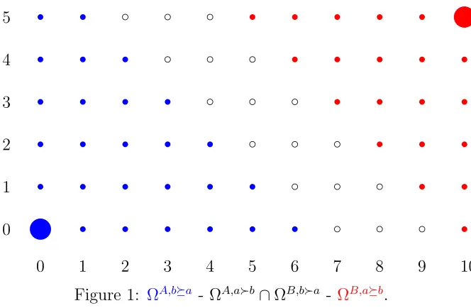
={(10,5),(3/5,2/3)}. (This is also the example covered in Section2.) Figure1 shows the state space Ω as an 11×6 lattice, with [ω]A ∈ {0, . . . ,10} on the horizontal-axis, and [ω]B ∈ {0, . . . ,5} on the vertical-axis. Each state is depicted by a circle.
Figure 1 is also a preference map, with ΩA,ba,ΩB,ab,ΩA,ab ∩ΩB,ba as the colour-coded partition of Ω. The set of blue circles is ΩA,ba, while the red circles
denote ΩB,ab. At the states depicted by hollow circles, the set ΩA,ab∩ΩB,ba, group
preferences disagree (by Lemma 1, GroupA prefers a, Group B prefers b). These sets are defined by (nAa, nAb, nBa, nBb ) = (7,9,10,6), calculated using equations (5)-(8).
To understand Group-Darwinianism, consider the state (5,3) in Figure 1. Since (5,3) ∈ ΩA,ab ∩ ΩB,ba, it must be that Ψ (5,3) ∈ {6, . . . ,10} × {0,1,2}. Mono-tonicity is also easily understood. Consider the pair of states, (5,2) and (5,3). Clearly (5,3)>a(5,2), and so Ψ (5,3)>aΨ (5,2). Since (5,2)∈ΩA,ab∩ΩB,ba, by Group-Darwinianism, Ψ (5,2)
∈ {6, . . .10} × {0,1}. If Ψ (5,3)
= (7,1), then monotonicity further restricts Ψ (5,2) to lie in the set {(6,1),(7,0),(7,1)}.
A large circle denotes a rest point of the dynamics. By Theorem 1, corner states
ωbb and ωaa are always rest points, while corner state ωab is also if the conditions of
part4 are satisfied. While states (nA
a −1,0) and (NA, NB−nBb + 1) can be rest points
nongenerically, no other state can be. Example 1 is both generic and the conditions
of Theorem 1 part 4 are not satisfied. So in Figure 1, the only two rest points are
~ s s s s s s s s s s s s s s s s s s s s s s s s s s c c c c c c c c c c c c c c c c c c s s s s s s s s s s s s s s s s s s s s ~ 0 1 2 3 4 5
0 1 2 3 4 5 6 7 8 9 10
Figure 1: ΩA,ba - ΩA,ab∩ΩB,ba - ΩB,ab.
and ΩB,ba, the colouring scheme for these states also connotes the rest point to which
they will lead.
Figure1 is not a complete description since it does not depict basins of attraction.
To partition Ω into {V(ω)}ω∈Ω
0, further information on the details of the dynamics is needed. To see how these details can matter, consider again state (5,3) in Figure 1. When Ψ = (BA,BB), the dynamics terminate at (10,5) via the path {(5,3) → (10,0)
→ (10,5)}. When Ψ = (ΨA
1,ΨB3), state (5,3) leads to (0,0), via the path {(5,3) →
(6,0)→(5,0)→(4,0)→(3,0)→(2,0)→(1,0)→(0,0)}.
Appendix B shows in detail how to construct basins of attraction for arbitrary
parameters when the groups respond at constant rates. While this requires some
nota-tion, the analysis has an intuitive graphical interpretation. Essentially, the procedure
amounts to conducting the analysis done on state (5,3) in the previous paragraph, for all states in ΩA,ab ∩ΩB,ba. Generically it is true that ΩA,ba ⊆ V(ωbb) and ΩB,ab
⊆ V(ωaa), so only states in ΩA,ab ∩ΩB,ba need be considered. Examples 2 and 3
below compute the basins of attraction for two separate dynamics for the parameters
of Example1.
Example 2(Basins of attraction when Ψ = (BA,BB)). From Figure 1, the situation is
clear: no matter what the current state, the following state must beωbb, ωab, orωaa. Blue
states jump immediately toωbb, black states toωab, and red states toωaa. Formally, for
anyω∈ΩA,ab∩ΩB,ba,B(ω) =ωab andB2(ω) =ωaa. That is, states in ΩA,ab∩ΩB,ba
transition first to ωab, and from there to ωaa, and so with Ψ = B, are part of V(ωaa).
ThusV(ωbb) = ΩB,ba and V(ωaa) = ΩA,ab∪(ΩA,ab∩ΩB,ba) = ΩB,ab.
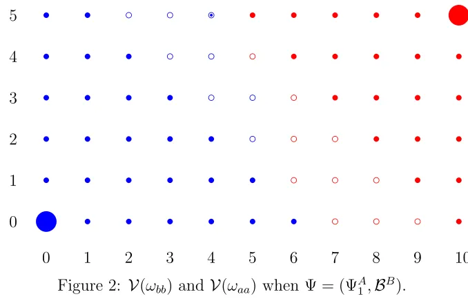
Example 3 (Basins of attraction when Ψ = (ΨA
1,ΨB3)). Figure 2 is not a preference
map. It colour-codes the basins of attraction, but also contains additional detail
illus-trating the recursive nature of the procedure used to construct them.
I show how to constructV(ωbb) from the ground up while glossing over some tedious
technical details. (AppendixB deals with these details.) Since ΨB
d ΨA, the
proce-dure says to begin by considering ΩA,ba ⊆ V(ωbb). The recursive part is as follows:
any state that maps to ΩA,ba must be part of V(ωbb); but then so must any state that
maps to any state that maps to ΩA,ba; but then so must ..., etc.
Begin by considering the upper boundary (ΩA,ba)+={ω| [ω]A+ [ω]B = 6}.
Con-sider those statesω∈ΩB,ba∩ΩA,absuch that Ψ(ω)∈(ΩA,ba)+. Call this set of states,
X, and consider the down set generated by it, X↓. Now define B1 := ΩA,ba ∪ X↓.
This appends the set{(2,5),(3,4),(3,5),(4,3), (4,4),(5,2),(5,3)}to ΩA,ba. In Figure 2these states are denoted by a hollow blue circle. But now, any stateω∈ΩB,ba∩ΩA,ab such that Ψ(ω) ∈ (B1)
+ must be part of V(ωbb).14 State (4,5) is the only state that
satisfies the requirement. This state is denoted by a hollow blue circle containing a
smaller solid blue circle in order to differentiate it. Since no states map to (4,5) under Ψ, it must be that all remaining states in ΩB,ba∩ΩA,ab are part ofV(ωaa) and so we
are done. These remaining states are denoted by a hollow red circle.
We can also trace how the boundaries of a basin of attraction vary. When ΨA∼ dΨB,
a basin of attraction’s boundaries and total boundaries will coincide.15 By Lemma 3,
for any monotone dynamics the basins will be convex. Extrapolating from Figure1, for
any Ψ such that ΨA∼ dΨB,
• V(ωbb)
+= V(ωbb)
++={(1,5),(2,4),(3,3),(4,2),(5,1),(6,0)} • V(ωaa)
− = V(ωaa)
−− ={(2,5),(3,4),(4,3),(5,2),(6,1),(7,0)}
while in Figure2, with Ψ = (ΨA
1,ΨA3), • V(ωbb)
+={(4,5),(5,3),(6,0)}
14The procedure is simplified by noting that actually only states inX↓\ΩA,ab need be considered.
15In fact, this statement also holds true under the condition thatξA≥nA
~ s s s s s s s s s s s s s s s s s s s s s s s s s s q c c c c c c c c c c c c c c c c c c s s s s s s s s s s s s s s s s s s s s ~ 0 1 2 3 4 5
0 1 2 3 4 5 6 7 8 9 10
Figure 2: V(ωbb) and V(ωaa) when Ψ = (ΨA1,BB).
• V(ωbb)
++={(4,5),(4,4),(5,3),(5,2),(5,1),(6,0)} • V(ωaa)
− ={(5,4),(6,1),(7,0)}
• V(ωaa)
−− ={(5,5),(5,4),(6,3),(6,2),(6,1),(7,0)}
5
Equilibrium Selection
Any deterministic Group-Darwinian dynamic, Ψ, induces a time-homogeneous Markov
process on the finite state space Ω. LetP be the associated transition matrix.16 That is,
for every pair of statesω0, ω00 ∈Ω,P(ω0, ω00)≥0 denotes the probability of transitioning fromω0 toω00, and for each ω∈Ω,P
ω0P(ω, ω0) = 1.
Let 4(Ω) denote the set of distributions on Ω. A stationary distribution of P is a row-vectorµ∈ 4(Ω), such thatµP =µ. The set of stationary distributions is denoted
40(Ω). Writing Pt for the t-fold application of P, and supp(µ) for the support of µ,
say that D ⊆ Ω is a recurrent class of P, if for all ω ∈ Ω, and all µ ∈ 4(Ω) with supp(µ) ⊆ D, limt→∞µPt
(ω) > 0 ⇐⇒ ω ∈ D. A state is recurrent if it is an element of a recurrent class, and transient otherwise. A singleton recurrent class is
anabsorbing state. For the Language Game, all recurrent classes are absorbing states,
corresponding with the rest points Ω0, as defined in Section 4.
All Markov processes possess at least one stationary distribution, while ergodic
Markov processes possess only one. The third assumption of KMR, perturbs the
deter-ministic dynamics in such a way as to induce a new Markov process that is ergodic.17
Assumption 3. Behavioural mutation: There is a small probability that an agent may
choose an action at random.
Specifically, after afforded decisions have been taken, but before payoffs are made,
with probability εA > 0 (εB > 0) each Group A (B) player switches his/her current
action, and with probability 1−εA (1−εB) maintains it.18
For constant rate dynamics, I claimed that there were no grounds for always
as-suming ΨA∼
d ΨB. Similarly, there is no reason to suppose that behavioural mutations
occur with equal likelihood for the different groups.19 But, while ultimately interest
will lie in the case where (εA, εB) ↓ (0,0), I will make the strong assumption that
εA = εB = ε, for all states and all time periods. It is tempting to insist on a milder
condition likeεA =O(εB) andεB=O(εA),20 but the equilibrium selection results may
differ.21
Mutations of size ε > 0 induce a new, ergodic Markov process with associated transition matrixPεand unique stationary distributionµε. Consider a sequence of such transition matrices {Pε}ε>0, each with corresponding stationary distribution {µε}ε>0. By continuity, the accumulation point of {µε}
ε>0, µ?, is a stationary distribution of
P := limε↓0Pε. Interest lies in the states to which µ? assigns positive probability. Definition 7. Stateω isstochastically stable, orselected, ifµ?(ω)>0, and uniquely so
if µ?(ω) = 1. Let Ω? denote the set of stochastically stable states.
17Actually this assumption makes the processirreducible andaperiodic, but for finite state Markov
processes this is sufficient for ergodicity. SeeKarlin and Taylor(1975).
18This interpretation is qualitatively different, though technically identical, to KMR’s interpretation. 19Nor is there any reason to suppose that mutations are both state- and time-independent. The
effects that subtle differences in mutation rates can have on equilibrium selection in general settings are discusses in detail inBergin and Lipman (1996).
20Letting both εA andεB be functions of ε, εA(ε) =O εB(ε)
as ε↓0, if and only if there exists positive numbersM andδ, such thatεA(ε)≤ |M εB(ε)|for allε < δ.
Calculating µ? is the objective. This is done using tree-surgery techniques from
Freidlin and Wentzell (1998), first introduced to game theory in Foster and Young (1990). To do so, consider states in Ω as the vertices of a fully connected directed
graph, Γ?. An edge in Γ? from ω0 to ω00 is denoted (ω0 → ω00). A path from ω0 to ω00
is a sequence of edges{(ωi →ωi+1)}
m−1
i=0 where ω0 =ω0, and ωm =ω00, and all vertices
are distinct. A typical path from ω0 to ω00 is denoted by h(ω0, ω00), and the set of all paths from ω0 to ω00 byH(ω0, ω00). Using this, the set of all paths from a state ω to a setQ63ω, H(ω, Q), can be defined as follows, H(ω, Q) :=∪ω0∈QH(ω, ω0).
Let k,k denote the taxicab metric (L1 distance) on Ω. For any pair ω0, ω00, define
cΨ(ω0, ω00) := kΨ(ω0), ω00k. The mapping cΨ : Ω×Ω → {0, . . . , N} is known as a cost function. The value it takes for any pair (ω0, ω00) is the minimum number of simultaneous mutations needed to transition directly fromω0 toω00 when the dynamics are described by Ψ. In graph theoretic terms, this is the cost of edge (ω0 →ω00) in Γ?.22
For any functionτ : Ω→Ω, a path from ω0 toω00 inτ, is a path{(ω0 →ω1),(ω1 →
ω2), . . . ,(ωm−1 → ωm)}, where ω0 = ω0 and ωm = ω00, such that τ(ωi) = ωi+1 for all
i = 0, . . . , m−1. An ω-tree, τω, is a mapping τω : Ω → Ω such that: (i) τω(ω) = ω;
(ii) for every ω0 ∈ Ω\ {ω}, there is a unique path in τω fromω0 to ω. Say that ω00 is a
successor of ω0 in τω if τωm(ω
0) = ω00 for some m ≥ 1, and the immediate successor if
m= 1.
For each ω, let Tω denote the set of all ω-trees. The cost of τω ∈ Tω is the sum of
costs of its edges,
cΨ(τω) = X
ω06=ω
cΨ ω0 →τω(ω0)
Define the set of states that achieve minimum cost ω-trees as Ξ(G, cΨ) :=
n
ω? ∈Ω
for any ω ∈Ω,τmin ω?∈Tω?
cΨ(τω?)≤ min τω∈Tω
cΨ(τω) o
The following is the result of Freidlin and Wentzell (1998) as applied to the Language Game. Note it’s relation to Definition 7above.
Lemma 4. Stateω is stochastically stable, or selected, if ω ∈Ξ(G, cΨ), and uniquely
so if {ω}= Ξ(G, cΨ). That is, Ξ(G, cΨ) = Ω?.
22In more general settings,c
Ψ can take any value inR+∪ {∞}, where∞is the value if a transition
By Theorem 4 of Young (1993), the stochastically stable states are contained in a recurrent class, which in this case are the absorbing states, Ω0. The key to computing
minimum costω-trees of the absorbing states, is to find paths of minimum cost between all pairs of them. Since, V(ω0)∩ V(ω00) = ∅ for all distinct ω0, ω00 ∈ Ω0, this amounts
to finding paths of minimum cost from each absorbing state to the convex basin of
attraction of the others. Before doing this, we need to know the precise structure of
the basins of attraction. Appendix B does this formally, though the procedure was
sketched in Examples 2and 3.
The two main results of the paper, Theorems2and3, concern equilibrium selection.
They compute the stochastically stable equilibria for the case whereE(G) = {ωbb, ωaa}
and E(G) = {ωbb, ωab, ωaa} respectively. Lemma 8 in Appendix C is needed for both
results. Lemma8says that a path of minimum cost out of a region of the state space in
which the dynamics are unambiguous, involves a direct transition out. An immediate,
and, for my analysis, the important consequence, is that it holds for the symmetric
profilesωbb and ωaa.
The analysis of each case is quite different, but the case whereE(G) ={ωbb, ωab, ωaa}
uses intuition that is more easily described in the first case and so I begin with it.
5.1
Equilibrium set is
{
ω
bb, ω
aa}
The main result in this section, Theorem 2, has a nice geometric interpretation that I
will explain before the formal statement. Refer back to Figures 1 and 2 which regard
the parameters from Example 1. From equation (5), nA
a = 7 ≤ NA, and therefore
ωab = (10,0)∈ V(ωaa). Figure1, with the hollow states assumed to be red, represents
the basins of attraction when ΨA ∼
d ΨB. In this case, a minimum cost ωaa-tree has
cost of 7 - one candidate costly edge being (0,0)→ (7,0)
. A minimum cost ωbb-tree
has cost of 9 - one candidate costly edge of the path being (10,5) → (1,5).23 Thus when ΨA∼d ΨB, clearly ωaa is the stochastically stable outcome.
Now look at Figure 2 representing the basins of attraction when Ψ = (ΨA
1,ΨB3).
As described in Section 4.2, the greater rate of adapting for Group B means that
V(ωbb) “eats” in to the region ΩA,ab ∩ΩB,ba. The cost of a minimum cost ωaa-tree
23Some work is required to show this since the path “jumps” through part of the region where
is unchanged, since the transition (0,0) → (7,0), is still available as an edge on a path from ωbb to V(ωaa). However, the minimum cost ωbb-tree is now different. Now
the transition (10,5)→(4,5)
is the unique costly edge on the path of minimum cost
fromωaa toV(ωbb). This has a cost of 6. The stochastically stable equilibrium changed
fromωaa to ωbb.
The following theorem performs this computation for any parameters.
Theorem 2. Suppose Condition 4 of Theorem 1 does not hold, so E = {ωbb, ωaa},
and that the monotonic Group-Darwinian adjustment process is such that both groups
evolve at constant rates. Let τ?
ωbb and τ ?
ωaa, denote minimum cost ω-trees for ωbb and
ωaa respectively. Then,
1. if (NA,0) = ω
ab∈ V(ωaa), then
cΨ(τω?aa) =n A
a, (15)
cΨ(τω?bb) =n A b −
(V(ωbb))+
N W , (Ω A,ba
)+
N W
; (16)
2. if (NA,0) = ωab∈ V(ωbb), then
cΨ(τω?bb) = n B
b , (17)
cΨ(τω?aa) = n B a −
(V(ωaa))−
N W , (Ω A,ba
)−
N W
. (18)
The set of stochastically stable states are those with the ω-tree of minimum cost. Proof. The proof is found in AppendixC.
Example 1 falls into case1 of the theorem. Some general statements can be made.
First, the state ωab plays an important role. When it is not an equilibrium, it always
lies in the basin of attraction of the larger group’s preferred convention. If the larger
group is weakly more reactive, then the region where preferences disagree will be part
of that group’s basin of attraction, and the larger group’s preferred outcome will be
stochastically stable. Furthermore, the feature whereby the minimum cost ωaa-tree is
unchanged from the example is robust, as it is always unchanged by varying dynamics
So when Group A is the larger group, the minimum cost ωaa-tree is nAa (since
(nA
a,0)∈ V(ωaa) always). The upper bound for a minimum cost ωbb-tree is nAb is given
in Equation (16). The second term in Equation (16) can be thought of as having an
indicator function in front, such that it only “kicks in” when GroupB is more reactive. This term computes the cost by which the minimum cost ωbb-tree is reduced from nAb.
A lower bound for the minimum cost ωbb-tree is given by nBb . This means that
Group B, the smaller group, must not only react quicker, but also have stronger rela-tive preferences for its preferred equilibrium to be stochastically stable. Conversely, if
GroupA, the larger group, has equally strong preferences, then (a,a) will always be a stochastically stable state.
5.2
Equilibrium set is
{
ω
bb, ω
ab, ω
aa}
Again, I will work through an example and then state the theorem. The example is a
variant ofG1 from Example1, where the size of the groups have been altered.
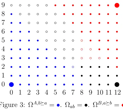
Example 4. LetG2 = (12,9,3/5,2/3). For these parameters E(G2) ={ω
bb, ωab, ωaa}.
Using equations (5) - (8), we get that (nAa, nAb, nBa, nBb ) = (9,13,14,8).
The state space forG2is a 13×10 grid, as depicted in Figure3. The first thing to note
is that regardless of rates of reaction, there exist some states at which the dynamics are
unambiguous. These states are represented by solid circles in Figure3, and are colour
coded by the convention to which they lead. The blue states represent ΩA,ba, the red
states comprise ΩB,ab, and the black states define the set Ωab ⊂(ΩA,ab ∩ΩB,ba), as
defined at the beginning of the proof of Theorem3. The remaining states are depicted
as hollow circles but they are also colour coded. State (7,2) is hollow and blue, because, depending on the dynamics, it can be an element ofV(ωbb) or V(ωab), but not V(ωaa).
Similarly, the hollow red circles, states (8,3),(8,4),(8,5),(9,3),(9,4), and (10,3), are so coloured since no matter what the dynamics, they cannot be elements ofV(ωbb). The
black hollow circles can be elements of any basin depending on the dynamics.
To solve for the stochastically stable states, we need to compute paths of
min-imum cost between the six pairs, (ωbb, ωab), (ωbb, ωaa), (ωab, ωbb),(ωab, ωaa),(ωaa, ωbb),
and (ωaa, ωab). Using Lemma 8, a minimum cost path over all h0 ∈ H(ωbb, ωab), has
edge of positive cost ωbb→(nAa,0)
w r r r r r r r r r r r r r r r r r r r r r r r r r r r r r r r r r r r r r r r r r r r r r r b b b b b b b b b b b b b b b b b b b b b b b b b b b b b b r r r r r r r r r r r r r w b b b b b b r r r r r r r r r r r r r r r r r r r r r r r r r r r r r r r r r r r rw 0 1 2 3 4 5 6 7 8 9
0 1 2 3 4 5 6 7 8 9 10 11 12
Figure 3: ΩA,ba=•. Ωab =•. ΩB,ab =•.
The cost of this path isnA
a (= 9). A similar statement holds for a path of minimum cost
fromωaa to ωbb, which has cost nBb (= 8), with costly edge ωaa →(NA, NB−nBb )
.
Lemma 10, in the Appendix, is essentially the analog of Lemma 8 for states in Ωab
(the solid black states in Figure3). Lemma 10is used to show that the unique path of
minimum cost fromωab toωbb has costly edge ωab →(NA−(nAb −NB),0)
with total
cost nA
b −NB (= 4). Similarly, the path of minimum cost from ωab to ωaa has costly
edge ωab →(NA, nBa −NA)
with total cost nB
a −NA (= 2).
The last two pairs to be considered are (ωbb, ωaa) and (ωaa, ωbb). An upper bound
for the paths of minimum costs between these can found by combining paths computed
above. For example, the path of minimum cost fromωbbtoωaa, must have cost at most
equal to nA
a + (nBa −NA) = 11. Lower cost paths between symmetric conventions can
be found when the dynamics are varied, but not when the groups react at equal rates.
This is stated formally in the following Theorem, whose proof is in AppendixC.
Theorem 3. Suppose Condition 4 of Theorem 1 holds, so E(G) ={ωbb, ωab, ωaa}, and
that the monotonic Group-Darwinian adjustment process is such that both groups evolve
at constant and equal rates. Let τω?bb, τω?ab, and τω?aa, denote minimum cost ω-trees for
ωbb, ωab, and ωaa respectively. Then,
cΨ(τω?bb) =n B b + (n
A b −N
B) (19)
cΨ(τω?ab) =n B
b +nAa (20)
cΨ(τω?aa) =n A a + (n
B a −N
A
The set of stochastically stable states are those equilibria withω-tree of minimum cost.
When the groups react at equal rates all hollow states in Figure 3 are part of
V(ωab). Let’s now apply Theorem 3. Plugging in to equations (19) - (21), we get that
cΨ(τω?bb), cΨ(τ ?
ωab), and cΨ(τ ?
ωaa) have costs 12 (= 8 + 4), 17 (= 9 + 8), and 11 (= 9 + 2) respectively. So when ΨA∼dΨB, conventionωaa is stochastically stable.
This is a good time to mention a few features of the set up. Due to the 2-dimensional
nature of the state space, there need not be a connection between the size of the basins
of attraction and stochastic stability.24 In fact, it is possible that the equilibrium with
the smallest basin of attraction is stochastically stable. To illustrate this refer back
to Figure 3 once again. When ΨA ∼d ΨB, simple counting yields |V(ωbb)| = 45,
|V(ωab)|= 44, and |V(ωaa)|= 36. We saw already thatωaa is stochastically stable, and
this is despite it having the maximal basin of attraction.
Another observation concerns the notions of the radius and modified coradius of a
recurrent class, introduced by Ellison (2000). The radius is defined as the minimum
number of mutations necessary to escape the basin of attraction, while the modified
coradius is defined as the maximum (over all states) of the minimum cost of a path
necessary to reach it, where one subtracts from the cost the radii of the intermediate
recurrent classes through which the path passes. Ellison (2000) shows that when the radius of a recurrent class is strictly greater than its modified coradius, this recurrent
class contains a stochastically stable state. Though the result is not universally powerful
as it only provides sufficient conditions, it does hold for many of the most frequently
studied games. In the Language Game, however, it need not be applicable whenE(G) =
{ωbb, ωab, ωaa}. Example4with ΨA∼dΨBdisplays this. The [radius, modified coradius]
pair for each absorbing state is given as follows, ωbb 7→[9,10], ωab 7→[2,9], and ωaa 7→
[8,9]. Note that all absorbing states have a greater modified coradius than radius. I now show (Theorem 4) that if ωab is stochastically stable when ΨA ∼d ΨB, then
the set of stochastically stable equilibria is independent of the specifics of the dynamics.
What happens is this. First, varying rates of adjustment will never lower the cost τω?
ab. Showing this is straightforward. Second, while it may lower the cost ofτ?
ωbb orτ ? ωaa, it will not lower the cost enough to alter selection. That is, Theorem4 does not say that
the minimum cost ω-tree of each convention is necessarily unchanged and as given by equations (19) - (21). Rather it just says that if ωab is ever stochastically stable for
some constant rate dynamic, it will always be for any constant rate dynamic and it will
haveω-tree with cost given by that in equation20.
Theorem 4. Suppose Condition4of Theorem 1holds, so E ={ωbb, ωab, ωaa}, and that
the monotonic Group-Darwinian adjustment process is such that both groups evolve at
constant rates. Ifωab ∈Ξ(G, cΨ) whenΨA∼dΨB, thenωab ∈Ξ(G, cΨ) for any constant rate Group-Darwinian adjustment processΨ.
Proof. The proof is found in AppendixC.
To reiterate, Theorem 4 does not say that equilibrium selection is unaffected by
varying rates. To see this, again consider Example4 and suppose that Ψ = (ΨA1,BB).
In Figure 3, all the hollow blue and black states are then elements of V(ωbb), and all
the hollow red states are elements ofV(ωab). The minimum cost ω-trees forωab andωaa
are unchanged. However, a new minimum costωbb-tree is attained with costly branches
ωab → (12,2)
and ωaa → (4,9)
, for a total cost of 10. Thus the stochastically
stable equilibrium is now ωbb. A formal result of this form would be similar to that of
Theorem3. The difference would appear in the analogs to equations (19) and (21). The
minimum cost ω-tree for ωbb, for example, would be the minimum of that in equation
(19), and the sum of (nB
a −NA) and a term similar to k (V(ωbb))+
N W, ωaak. While
this second term’s value must be at least nB
b , slightly more care must be taken since it
need not be the case that ωba ∈ V(ωbb). And a statement like that of Lemma 9 need
not hold true in this case.
6
Stability versus Welfare
When the population is homogeneous, players collectively agree on what action they
“would like to have taken” earlier today, and hence what action they will choose for
tomorrow if afforded a revision opportunity. The main issue in existing large population
coordination problems is the tension between efficiency and risk-dominance. Both KMR
and Young (1993) show that the risk-dominant action will emerge under perturbed best-response based dynamics. This result isnegative in the sense that the locally
risk-dominant equilibrium action need not coincide with the Pareto-risk-dominant one, and may
In the Language Game, both symmetric profiles are Pareto-efficient equilibria, and
there is never uniform preference over these. Thus Pareto-efficiency is useless as a
selection device. The purpose of this section is to rank profiles in E(G) according to various welfare criteria, and then compare this ranking to the outcome(s) selected by
decentralised dynamics. Since all profiles in E(G) are group-symmetric, to infer how members of the population rank them, it suffices to analyse the situation from the
perspective of any one agent from each Group.
Theorem 5. Within the set of group-symmetric profiles:
1. ωaa and ωbb are always Pareto-efficient.
2. ωab is Pareto-efficient if and only if
p≥ N −1
2N −NB−2 and q≥
N−1
2N −NA−2 (22)
Proof. The proof is straightforward and is omitted.
A natural question to ask is the relationship between Pareto-efficiency and
equilib-rium. The following shows that a Pareto-efficient profile must be an equilibrium, but
that not all equilibria are Pareto-efficient.
Theorem 6. If ωab is Pareto-efficient, then it must be an equilibrium. Butωab may be
an equilibrium without being Pareto-efficient.
Proof. Follows from conditions in part4of Theorem1, and those in part 2of Theorem
5. The second imply the first, while the first need not imply the second.
Consider another variant of G1 from Example 1, in which Group B’s preference
for coordinating on action b are stronger. Specifically, consider the new game G3 =
(10,5,3/5,5/6). In this case, E(G3) = {ω
bb, ωab, ωaa}. Evaluating utilities at each
equi-librium givesUA(ω
aa), UB(ωaa) ={42/5,28/6},
UA(ω
ab), UB(ωab) ={27/5,50/6},
and {UA(ω
bb), UB(ωbb)} = {28/5,140/6}. Note that ωab is Pareto-dominated by ωbb,
and so provides an example of Theorem6 at work.
It can be checked thatωab is not a stochastically stable inG3. One might then
won-der whether or not stochastic stability will ever select a Pareto-inefficient convention.
Theorem 7. Suppose E(G) = {ωbb, ωab,