Vol. 9, No. 1, 2017 Article ID IJIM-00584, 6 pages Research Article
A New Approach for Solving Volterra Integral Equations Using the
Reproducing Kernel Method
R. Ketabchi ∗, R. Mokhtari†, E. Babolian ‡§
Received Date: 2014-09-01 Revised Date: 2014-10-27 Accepted Date: 2016-08-03 ————————————————————————————————–
Abstract
This paper is concerned with a technique for solving Volterra integral equations in the reproducing kernel Hilbert space. In contrast with the conventional reproducing kernel method,the Gram-Schmidt process is omitted here and satisfactory results are obtained. The analytical solution is represented in the form of series. An iterative method is given to obtain the approximate solution. The convergence analysis is established theoretically. The applicability of the iterative method is demonstrated by testing some various examples.
Keywords: Reproducing kernel method; Volterra integral equations; Gram-Schmidt orthogonalization process.
—————————————————————————————————–
1
Introduction
I
nmethod (RKM) has been a promising methodthe last decades, the reproducing kernel which applied more and more for solving vari-ous problems such as ordinary differential equa-tions, partial differential equaequa-tions, differential-difference equations, integral equations, and so on (see e.g. [1]-[16] and references therein). Among many literatures related to RKM for solving var-ious problems and even among a bunch of exten-sive works related to RKM for solving integral equations, we just mention some more interest-ing problems. An approximate solution of the Fredholm integral equation of the first kind in∗Department of Mathematics, Science and Research branch, Islamic Azad University, Tehran,Iran.
†Department of Mathematical Sciences, Isfahan Uni-versity of Technology, Isfahan 84156-83111, Iran.
‡Corresponding author. [email protected], Tel: +98 (21)77630040.
§Department of Mathematics, Science and Research branch, Islamic Azad University, Tehran, Iran.
the reproducing kernel space was presented by Du and Cui [8,9], solution of a system of the lin-ear Volterra integral equations was discussed by Yang et al. [10], solvability of a class of Volterra integral equations with weakly singular kernel us-ing RKM was investigated in [11, 12, 13], Geng [14] explained how to solve a Fredholm integral equation of the third kind in the reproducing ker-nel space, and Ketabchi et al. [7] obtained some error estimates for solving Volterra integral equa-tions using RKM. In [7] and some other places, a general technique for solving Volterra integral equations was discussed in the reproducing ker-nel space. This general technique is based on the Gram-Schmidt (GS) orthogonalization pro-cess. In this study, we aim to explain how to construct a reproducing kernel method without using this process. For this purpose, we consider the following nonlinear Volterra integral equation
u(x) =F(x, u(x)), (1.1)
where
F(x, u(x)) =f(x) +
∫ x
0
k(x, ξ)N(u(ξ))dξ,
x ∈ [0,1], in which functions f and k and the nonlinear operator N are considered such that Eq. (1.1) has a unique solution. Furthermore, we need to assume that F is continuous. The rest of the paper is organized as follows. In the next Section, some preliminaries are represented. The method implementation is discussed in Section3. Section4is devoted to convergence analysis of the method. For confirming the theoretical results, some numerical examples are provided in Section
5. The paper will be closed by a brief conclusion in the last Section.
2
Preliminaries
In this section, we follow the recent work by Cui et al. [16] and represent some useful materials.
Definition 2.1 LetH be a Hilbert space of func-tions f : Ω → R. Denote by < ., . > the in-ner product and let ∥.∥=√< ., . >be the induced norm in H. The function R : Ω×Ω → R is called a reproducing kernel of H if the followings are satisfied
(i) Ry(x) =R(x, y)∈H,∀y∈Ω,
(ii) f(y) =< f(x), Ry(x)>,∀f ∈H, for all y ∈ Ω.
Definition 2.2 A Hilbert space H of functions on a set Ω is called a reproducing kernel Hilbert space if there exists a reproducing kernel R of H.
Remark 2.1 The existence of the reproducing kernel of a Hilbert space is due to the Riesz Rep-resentation Theorem. It is known that the repro-ducing kernel of a Hilbert space is unique.
Theorem 2.1 [5] The reproducing kernel R of reproducing kernel Hilbert spaceH is positive def-inite.
Definition 2.3 The function space Wm[0,1] is defined as follows
Wm[0,1] = {u|u(m−1) ∈ AC[0,1], u(m) ∈
L2[0,1]},
AC[0,1] is an absolutely continuous function in [0,1].
The inner product and norm in Wm[0,1] are de-fined respectively by
< u, v >Wm=
=∑mi=0−1u(i)(0)v(i)(0) +∫01u(m)(x)v(m)(x)dx,
∀u, v∈Wm[0,1],
∥u∥Wm=
√
< u, u >Wm,∀u∈Wm[0,1].
In general, the function space Wm[0,1] is a re-producing kernel space and its rere-producing ker-nel Rm has the following reproducing property
u(.) =< u(x), Rm(x, .)>Wm,∀u ∈ Wm[0,1]. For m= 1, the function space W1[0,1] is a reproduc-ing kernel space and its reproducreproduc-ing kernel is
R(x, y) =
{
1 +x, x≤y,
1 +y, x > y.
3
The method implementation
We rewrite Eq. (1.1) as follows
Lu(x) =f(x) +
∫ x
0
k(x, ξ)N(u(ξ))dξ,
where L : W1[0,1] → W1[0,1] is an invert-ible bounded linear operator, N is a nonlin-ear operator, and f is an arbitrary function in
W1[0,1].W1[0,1] is a reproducing kernel space de-fined according to the highest derivatives involved in (1.1).We choose a countable set of points {xi}∞i=1 in the interval [0,1], and define
ϕi(x) =R(x, xi), ψi(x) =L∗ϕi(x),
where L∗ is the adjoint operator of L.Obviously, in this paperLis the identity operator and there-fore ψi(x) =R(x, xi).
Theorem 3.1 Let {xi}∞i=1 be dense in the inter-val[0,1]. If Eq. (1.1) has a unique solution, then it can be represented as
u(x) = ∞ ∑
j=1
ajψj(x), (3.2)
where the coefficientsaj are determined by solving the following semi-infinite system of linear equa-tions
Ba=F, (3.3)
in which
B = [ψj(xi)], i, j= 1,2, . . . ,
a= [a1, a2, . . .]T, and
Proof. Since {xi}∞i=1 is dense in the interval [0,1], thenψj(x) is a complete system inW1[0,1], see e.g. [16]. So the analytical solution can be represented as Eq. (3.2). Since
< ψi(x), ψj(x)>w1= < L∗ϕi(x), ψj(x)>w1=
< ϕi(x), Lψj(x)>w1=Lψj(x)|x=xi=ψj(xi),
and
< u(x), ψj(x)>w1= < u(x), L∗ϕj(x)>w1=
< Lu(x), ϕj(x)>w1=F(xj, u(xj)),
according to the best approximation in Hilbert spaces [5], the coefficients aj are determined by (3.3).
The approximate solution of the problem is the
m-term intercept of the analytical solution which can be determined by solving am×msystem of linear equations. We need to construct an itera-tive method for solving (3.3). For this purpose, we choose the number of points m, the num-ber of iterations n and put the initial function
u0,m(x) = 0. Then, the approximate solution of Eq. (1.1) is defined by
un,m(x) = m
∑
j=1
anjψj(x) =F(xj, un−1,m(xj)).
(3.4)
Remark 3.1 There exists a unique solution for equations (3.4) due to the strictly positive defi-niteness property of the reproducing kernel.
The results of this section can be summarized in the following algorithm.
Algorithm1.
1. Choose m collocation points in the interval [0,1].
2. SetB = [ψj(xi)], i, j = 1,2, . . . , m.
3. Choose the number of iterationsn.
4. Seti= 0.
5. Set the initial functionu0,m(x) = 0.
6. Seti=i+ 1.
7. SetF = [F(xj, ui−1,m(xj))]T, j = 1, . . . , m.
8. Solve Ba=F.
9. Setui,m(x) =∑mj=1aijψj(x).
10. If i < n, then go to step 6, else stop the algorithm.
The conventional reproducing kernel method which used the GS orthogonalization process is represented in the following algorithm [7].
Algorithm2.
1. Choose m collocation points in the domain set [0,1].
3. Setψi(x) =R(x, xi), i= 1, . . . , m.
4. Set ¯ψi(x) =
∑i
k=1βikψk(x), i = 1, . . . , m, (βik which obtained by the GS process).
5. Choose an initial function u0(x).
6. Setn= 1.
7. SetBn=
∑n
l=1βnlF(xl, un−1(xl)).
8. Setun(x) =∑nj=1Bjψ¯j(x).
9. Ifn < m, then setn=n+ 1 and go to step 7, else stop.
Remark 3.2 In comparison with Algorithm 2, Algorithm 1 needs not to use the GS orthogonal-ization process but in step 8 of it, we must to solve a linear system. The coefficient matrix of this system is positive definite because of the positive definiteness of the kernel. Therefore, it needs to decompose matrix B once using the QR decom-position and to solve a triangular system in step 8.
4
Convergence analysis
In this section, we show that the approximate solution un,m is converged to the analytical solu-tion uuniformly. At first, the following lemma is given.
Lemma 4.1 For a positive constant M, A = {u| ∥u∥w1≤ M} is a compact set in the space C[0,1] provided that ∥u′∥w1≤c,
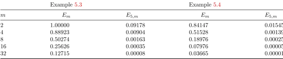
Table 1: Results of Algorithms 1 and 2.
Example5.1 Example5.2
m Em E5,m Em E5,m
2 2.71828 0.09544 1.00000 0.22222
4 1.33040 0.01045 0.97862 0.02663
8 0.69767 0.00187 0.69761 0.00478
16 0.35213 0.00036 0.40235 0.00103
32 0.17439 0.00005 0.21231 0.00024
Table 2: Results of Algorithms 1 and 2.
Example5.3 Example5.4
m Em E5,m Em E5,m
2 1.00000 0.09178 0.84147 0.01545
4 0.88923 0.00904 0.51528 0.00139
8 0.50274 0.00163 0.18976 0.00025
16 0.25626 0.00035 0.07976 0.00005
32 0.12715 0.00008 0.03665 0.00001
Proof. It is enough to show thatAis a bounded and equicontinuous set [5]. Since
∥R(x, y)∥2w1=
< R(x, y), R(x, y)>w1=R(x, x)< c0,
wherec0 is a positive constant, there exists a con-stantc1 such that
|u(x)|=|< u(y), R(x, y)>w1 |≤
∥u(y)∥w1∥R(x, y)∥w1≤c1∥u(y)∥w1.
For any u∈A, we have|u(x)|≤c1M HenceA is a bounded set in the space C[0,1]. On the other hand,
|u′(x)|=|< u(y),∂R∂x(x,y) >w1 |≤
∥u(y)∥w1∥∂R∂x(x,y)∥w1≤
c2∥u(y)∥w1≤c2M
Then for any u∈A and ϵ >0, we have |u(x+h)−u(x)|≤ |u′(η)||h|≤c2M|h|
where η ∈ [x, x+h]. So, there exists δ = cϵ
2M
such that for|h|< δ, we get|u(x+h)−u(x)|< ϵ
Hence A is an equicontinuous set in the space
C[0,1].
Theorem 4.1 If L is an invertible bounded linear operator and F(x, u(x)) is a nonlin-ear bounded operator, it can be deduced that {un,m(x)}∞n=1 is the bounded sequence of func-tions in w1[0,1].
Proof. We can write
∥un,m(x)∥2w1
=< un,m(x), un,m(x)>w1
=<∑mj=1ajψj(x),
∑m
l=1alψl(x)>w1
=∑mj=1aj < ψj(x),
∑m
l=1alψl(x)>w1
=∑mj=1aj < ϕj(x),
∑m
l=1alψl(x)>w1
=∑mj=1aj(
∑m
l=1alψl(xj)) =aTBa,
where
a= [aj], j= 1,2, . . . , m.
Now, since
B = [ψj(xi)], i, j= 1,2, . . . , m,
is a positive definite matrix then we have a =
B−1F and the assumed assumptions imply that ∥un,m(x)∥w1≤M,
where M is a constant.
Theorem 4.2 Assume that {xi}∞i=1 is dense in [0,1] and the assumptions of Theorem 4.1 and Lemma 4.1 hold. Then the approximate solution
un,m is converged to the analytical solutionu.
Proof. For j = 1,2, . . . , m and n = 1,2, . . ., we have Lun,m(xj) =F(xj, un−1,m(xj)).
According to Lemma 4.1, there exists a conver-gent subsequence {unl,m(x)}∞l=1 of {un,m(x)}∞n=1 such that unl,m(x) → un,m(x), uniformly as l →
∞, m → ∞. Then for j = 1,2, . . . , m and
n= 1,2, . . ., we derive
Since the operatorsLandF are both continuous (according to the structure of Land assumption onF), after taking limit from both sides of (4.5), it can be inferred that u is the analytical solu-tion of Eq. (1.1). Sounl,m(x) is the approximate
solution of Eq. (1.1).
5
Examples
In this section, we compare results of both Algo-rithms in solving four various problems using the following norms
∥u−un,m∥∞≃En,m= max
1≤i≤m|u(xi)−un,m(xi)|,
∥u−um∥∞≃Em = max
1≤i≤m|u(xi)−um(xi)|,
whereun,mandumare approximate solutions ob-tained by Algorithms 1 and 2, respectively andu
is the exact solution. The results of Tables 1, 2
(for n= 5) confirm the superiority of Algorithm 1.
Example 5.1 If k(x, ξ) =x2ξ, f(x) = exp(x)−
x2+x2exp(x)−x3exp(x) and N(u(x)) =u(x), then the Volterra integral equation (1.1) has the following exact solution u(x) = exp(x).
Example 5.2 Ifk(x, ξ) =x72ξ,f(x) =x 7 2−2
11x9 and N(u(x)) = u(x), then the Volterra integral equation (1.1) has the following exact solution
u(x) =x72.
Example 5.3 If k(x, ξ) = x2ξ, f(x) = 12x2 + 1
2x
2cos(x2) and N(u(x)) = sin(u(x)), then the
Volterra integral equation (1.1) has the following exact solution u(x) =x2.
Example 5.4 If k(x, ξ) = sin(x− ξ), f(x) = sin(x) +23cos(x)−16cos(2x)− 12 andN(u(x)) =
u(x)2, then the Volterra integral equation (1.1) has the following exact solution u(x) = sin(x).
6
Conclusion
In this work, we proposed an iterative algorithm for solving nonlinear volterra integral equations on the basis of the reproducing kernel Hilbert space without using the Gram-Schmidt orthog-onalization process.The results of some numeri-cal examples show that the present method could be an accurate and reliable analytical-numerical
technique.Examples presented here belong to dif-ferent categories such as linear or nonlinear prob-lem with smooth or none-smooth kernel and so-lution.Nevertheless, our results only apply to the given examples; this, of course, does not mean that it holds in general.The advantage of the ap-proach is that the method can be easily imple-mented. It seems that the method can be also applied for solving other nonlinear integral equa-tions.
References
[1] F. Z. Geng, M. G. Cui, Appl. Math. Letters, 25, 818-823 (2012).
[2] F. Z. Geng, S. P. Qian, Appl. Math. Letters, 26, 998-1004 (2013).
[3] M. Mohammadi, R. Mokhtari, J. Comput. Appl. Math., 235, 4003-4011 (2011).
[4] M. Mohammadi, R. Mokhtari, Iranian J. Sci. Tech. Trans. A., 37, 546-523 (2013).
[5] M. Mohammadi, R. Mokhtari,Math. Model. Anal., 19, 180-198 (2014).
[6] R. Mokhtari, F. Toutian Isfahani, M. Mo-hammadi, Abs. Appl. Anal., Article ID 514103 (2012).
[7] R. Ketabchi, R. Mokhtari, E. Babolian, J. Comput. Appl. Math., 273, 245-250 (2015).
[8] H. Du, M. G. Cui, Appl. Math. Letters, 21, 617-623 (2008).
[9] H. Du, M. G. Cui, Appl. Math. Comput., 182, 1608-1614 (2006).
[10] L. H. Yang, J. H. Shen, Y. Wang,J. Comput. Appl. Math, 236, 2398-2405 (2012).
[11] Z. Chen, W. Jiang, Appl. Math. Comput., 217, 7515-7519 (2011).
[12] Z. Chen, Y. Lin Y, J. Math. Anal. Appl., 344, 726-736 (2008).
[13] W. Jiang, M. G. Cui, Appl. Math. Comput., 202, 666-674 (2008).
[15] F. Z. Geng, S. P. Qian, S. Li, J. Comput. Appl. Math., 255, 97-105 (2013).
[16] M. G. Cui, Y. Lin, Nova Science Pub. Inc., Hauppauge, (2009).
Razieh Ketabchi is an Assistant professor at the Department of Mathematics in Islamic Azad Uni-versity Mobarakeh branch, IAU. She received PHD degree in ap-plied mathematics, numerical anal-ysis field from Science and Re-search Branch, Islamic Azad University. Her re-search interests include Numerical solution of IEs ODEs.
Reza Mokhtari is an Associate Pro-fessor in Numerical Analysis at the Isfahan University of Technology, Isfahan, Iran (IUT). He received PHD degree in Applied Mathe-matics (Numerical Analysis) from the Iran University of Science and Technology. His research interests include Nu-merical Analysis, Scientific Computing, Numer-ical solution of ODEs, PDEs IEs and Mesh-dependent Meshfree methods.