Vol. 6, No. 2, 2014 Article ID IJIM-00389, 5 pages Research Article
Solving Differential Equations Using Modified VIM
F. Goharee ∗ †, E. Babolian ‡
————————————————————————————————–
Abstract
In this paper a modification of He’s variational iteration method (VIM) has been employed to solve Duffing and Riccati equations. Sometimes, it is not easy or even impossible, to obtain the first few iterations of VIM , therefore, we suggest to approximate the integrand by using suitable expansions such as Taylor or Chebyshev expansions.
Keywords: Variational iteration method; Duffing equation; Riccati equation; Taylor expansion; Cheby-shev expansion.
—————————————————————————————————–
1
Introduction
T
happlied science. In this paper, we considere Duffing equation is a nonlinear equation of the nonlinear Duffing equation of the form{
u′′(t) +αu′(t) +βu(t) +γu3(t) =f(t)
u(0) =a, u′(0) =b.
(1.1) where α, β, γ, a, b are real constants. Vahidi et al. in [1] used the restarted Adomian’s decompo-sition method to solve Duffing equation, also in [2] they used homotopy perturbation method for solving nonlinear Duffing equations.
The general form of Riccati equation is as follows: {
u′(t) =A(t) +B(t)u(t) +c(t)u2(t), 0≤t≤T u(t0) =d.
(1.2)
where A(t), B(t), C(t) are given functions and
d is an arbitrary constant. The Riccati equa-tion plays an important role in some fields of
∗Corresponding author. [email protected]
†Department of Mathematics, Science and Research
Branch, Islamic Azad University, Tehran, Iran.
‡Department of Mathematics, Science and Research
Branch, Islamic Azad University, Tehran, Iran.
applied sciences. Recently, Adomian’s decom-position method has been employed for solv-ing Riccati differential equations in [3]. Geng [4] presented the piecewise VIM for solving Ric-cati differential equations. Abbasbandy [5, 6, 7] used He’s VIM, homotopy perturbation method (HPM) and iterated He’s HPM to solve this equa-tion. Here, we propose a modification of VIM and show by some examples that using this modifica-tion accurate solumodifica-tions can be obtained.
2
Outline of VIM
Variational iteration method plays an important role for solving different types of differential equa-tions [8,9,10,11,12,13,14,15,16].
To illustrate the basic idea of the method we con-sider the following nonlinear equation:
Lu(t) +N u(t) =g(t), (2.3)
where L is a linear operator, N is a nonlinear op-erator, and g is a known analytic function. Ac-cording to VIM, we can construct the following correction functional:
un+1(t) =
un(t) + ∫ t
0
λ(t, x){Lun(x) +Nuen(x)−g(x)}dx.
(2.4) where λ is a Lagrange multiplier, which can be identified optimally via the variational theory, and une is a restricted variation which means
δuen = 0. The successive approximation un(x); n ⩾ 1, of the solution u(x) will be readily ob-tained upon using the obob-tained Lagrange multi-plier and by using selective function uo(x).
Con-sequently, the exact solution maybe obtained by using
u(x) = limn→∞un(x),
when un(x) has a limit as n→ ∞.
3
Description of the Modified
VIM
In general the method of VIM only a few itera-tions can be applied for Duffing and Riccati equa-tions, because as we proceed the integrand in-volved on the right hand side of (2.4) becomes complicated. therefore, to achive a high accurate solution we replace the integrand by Taylor and Chebyshev expansions as follows:
1)Taylor expasion:
f(x)≈
n ∑
k=0
f(k)(0)
k! x
k. (3.5)
2)Chebyshev expansion:
f(x)≈ ∞
∑
i=0
aiTi(x), ai=
2
π ∫ 1
−1
f√(x)Ti(x)
1−x2 (3.6)
Here, we assume that all integrands have Taylor and Chebyshev expansions (3.5), (3.6).
4
Numerical Examples
In this section, we illustrate the proposed modi-fication of the Variational iteration method with three examples. All of the calculation have been done with Maple 15 with 8 digits precision.In all of examples, Chebyshev expansions, have been obtained with tolerance 10−10 and for all exam-ples only 10 terms of Taylor expansions have been used.
Example 4.1 Consider the following Duffing equation
{
u′′(t) + 2u′(t) +u(t) + 8u3(t) =e−3t
u(0) = 1/2, u′(0) =−1/2, (4.7)
with the exact solution u(t) = 12e−t.
According to VIM, we can construct the correc-tion funccorrec-tional of Eq. (4.7) as follows:
un+1(t) =un(t)+ ∫ t
0
λ{u′′n(x) + 2eu′n(x) +eun(x) + 8ue3n(x)−e−3x}dx.
(4.8) where λ is general Lagrange multiplier and
e
u′n(x),une (x),ue3n(x) denote restricted variations,
i.e.
δue′n(x) =δuen(x) =δue3n(x) = 0.
The stationary conditions yields:
1−λ′(x)
x=t= 0, λ(x)
x=t= 0,λ
′′(x)
x=t= 0,
hence, the Lagrange multiplier can be identified asλ=x−t.
Therefore, the following iteration formula is obtained:
un+1(t) =un(t)+ ∫ t
0
(x−t){u′′n(x)+2u′n(x)+un(x)+8u3n(x)−e−3x}dx.
(4.9) According to Eq. (4.7) initial approximation is
u0(t) = 12 − 12t and the numerical results are tabulated in Table 1, where by um(x) we mean
mthiteration of (4.9).
If we use VIM for (4.9), in the second iteration,
u2(t) is as follows:
−0.14139104t − 0.21682098t4 − 0.07206790t5 + 0.03271858e−3t+ 0.06851851t6−0.03747795t7−
0.09039351t8+ 0.05428240t9+ 0.00024691t10
−0.02451178t11+0.02002525t12−0.00912393t13+ 0.00269230t14−0.00052380t15+ 0.00006250t16−
0.00000367t17−0.26303155t2
+0.29526748t3 − 0.27942894te−3t −
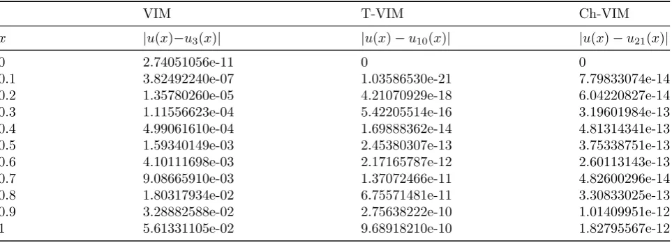
Table 1: Comparison of absolute errors for Example4.1, using VIM, Taylor-VIM, Chebyshev-VIM.
VIM T-VIM Ch-VIM
x |u(x)−u3(x)| |u(x)−u10(x)| |u(x)−u21(x)|
0 2.74051056e-11 0 0
0.1 3.82492240e-07 1.03586530e-21 7.79833074e-14 0.2 1.35780260e-05 4.21070929e-18 6.04220827e-14 0.3 1.11556623e-04 5.42205514e-16 3.19601984e-13 0.4 4.99061610e-04 1.69888362e-14 4.81314341e-13 0.5 1.59340149e-03 2.45380307e-13 3.75338751e-13 0.6 4.10111698e-03 2.17165787e-12 2.60113143e-13 0.7 9.08665910e-03 1.37072466e-11 4.82600296e-14 0.8 1.80317934e-02 6.75571481e-11 3.30833025e-13 0.9 3.28882588e-02 2.75638222e-10 1.01409951e-12 1 5.61331105e-02 9.68918210e-10 1.82795567e-12
0.40938881e−3tt2−0.34202103e−3tt3
−0.04074074e−3tt6 − 0.01358024e−3tt8 + 0.00246913e−3tt9 + 0.00164609e−3tt7 −
0.00074074e−3tt10 + 0.00106691te−6t + 0.00137174e−6tt4
−0.00041152e−6tt5 − 0.00114311e−6tt2 −
0.00274348e−6tt3+0.47019847−0.00278158e−6t−
0.00013548e−9t.
It is easy to see that, next iterations have more terms and become more complicated, therefore to overcome this difficulty we re-place the integrand by Taylor or Chebyshev expansions.
Example 4.2 Consider the following Duffing equation
{
u′′(t) + 3u(t)−2u3(t) =costsin2t
u(0) = 0, u′(0) = 1, (4.10)
with the exact solution u(t) =sint.
Similar to example (4.1) the iteration furmula for equation (4.10) is:
un+1(t) =un(t)+ ∫ x
0
(x−t){u′′n(x)+3un(x)−2u3n(x)−cosxsin2x}dx.
(4.11) According to Eq. (4.10) initial approximation is
u0(t) =tand the numerical results are tabulated in Table2.
Example 4.3 Consider the following Riccati equation
{
u′(t) = 1 + 2u(t)−u2(t), 0≤t≤1
u(0) = 0.48364861,
(4.12)
with the exact solution u(t) = 1 +√2 tanh(√2t+ 1
2log
√
2−1
√
2+1).
According to the variational iteration method, we can construct the correction functional of Eq. (4.12) as follows:
un+1(t) =un(t)+ ∫ t
0
λ{u′n(x)−2un(x)−1 +eu2n(x)}dx. (4.13)
whereλis general Lagrange multiplier andue2n(x) denote restricted variation, i.e. δue2n(x) = 0. The stationary conditions yields:
1 +λ(t, x)
x=t= 0, λ
′(t, x) + 2λ(t, x) = 0.
these equations yield:
λ=−e2(x−t).
and the iteration furmula for the Riccati equation is as follows:
un+1(t) =un(t)− ∫ x
0
e2(x−t){u′n(x)−1−2un(x) +u2n(x)}dx.
(4.14) According to Eq. (4.12) initial approximation is
Table 2: Comparison of absolute errors for Example4.2, using VIM, Taylor-VIM, Chebyshev-VIM.
VIM T-VIM Ch-VIM
x |u(x)−u2(x)| |u(x)−u5(x)| |u(x)−u6(x)|
0 0 0 0
0.1 1.67707847e-04 1.60582791e-23 9.13801475e-15 0.2 1.34604752e-03 1.31530632e-19 1.54481934e-14 0.3 4.59073661e-03 2.55923337e-17 4.25219661e-14 0.4 1.10152497e-02 1.07688356e-15 1.56458755e-14 0.5 2.17671868e-02 1.95800091e-14 4.77034519e-14 0.6 3.79382391e-02 2.09383174e-13 1.19483205e-13 0.7 6.04001929e-02 1.55232085e-12 2.34465586e-13 0.8 8.95609796e-02 8.80170983e-12 6.43658653e-13 0.9 1.25042472e-01 4.06629542e-11 8.18536342e-13 1 1.65288637e-01 1.59828525e-10 1.30343939e-13
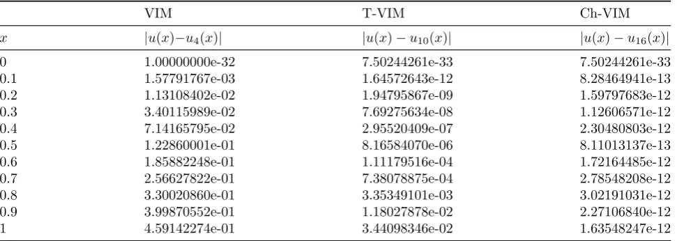
Table 3: Comparison of absolute errors for Example4.3, using VIM, Taylor-VIM, Chebyshev-VIM.
VIM T-VIM Ch-VIM
x |u(x)−u4(x)| |u(x)−u10(x)| |u(x)−u16(x)|
0 1.00000000e-32 7.50244261e-33 7.50244261e-33 0.1 1.57791767e-03 1.64572643e-12 8.28464941e-13 0.2 1.13108402e-02 1.94795867e-09 1.59797683e-12 0.3 3.40115989e-02 7.69275634e-08 1.12606571e-12 0.4 7.14165795e-02 2.95520409e-07 2.30480803e-12 0.5 1.22860001e-01 8.16584070e-06 8.11013137e-13 0.6 1.85882248e-01 1.11179516e-04 1.72164485e-12 0.7 2.56627822e-01 7.38078875e-04 2.78548208e-12 0.8 3.30020860e-01 3.35349101e-03 3.02191031e-12 0.9 3.99870552e-01 1.18027878e-02 2.27106840e-12 1 4.59142274e-01 3.44098346e-02 1.63548247e-12
5
Conclusion
In this paper, we presented a modification of VIM to solve Riccati and Duffing equations. This mod-ification is based on replacing the integrand, in-volved in the corresponding correction functional, by its Taylor or Chebyshev expansions. Numeri-cal experience show that using the proposed mod-ification one can obtain more accurate solutions, and the overall performance, when we use Cheby-shev expansion, is better.
References
[1] A. R. Vahidi, E.Babolian, Gh. Asadi Cord-shooli and F. Samiee, Restarted Adomian’s decomposition method for Duffing’s equation, J. Math. Anal. 3 (2009) 711-717.
[2] A. R. Vahidi, E. Babolian, A. Azimzadeh, An improvement to the homotopy perturba-tion method for solving nonlinear Duffing’s equations, Bulletin of the Malaysian Mathe-matical Sciences Society, (2011).
[3] M. A. El-Tawil, A. A. Bahnasawi, A. Abdel-Naby, Solving Riccati differential equation using Adomian decomposition method, Ap-plied Mathematics and Computation 157 (2004) 503-514.
[4] F. Z. Geng, Y. Z. Lin, M. G. Cui, A piece-wise variational iteration method for Riccati differential equations, Computers and Math-ematics with Applications 58 (2009) 2518-2522.
de-composition method, Applied Mathematics and Computation 172 (2006) 485-490.
[6] S. Abbasbandy, A new application of He’s variational iteration method for quadratic Riccati differential equation by using Ado-mian’s polynomials, Journal of Computa-tional and Applied Mathematics 207 (2007) 59-63.
[7] S. Abbasbandy,Iterated He’s homotopy per-turbation method for quadratic Riccati dif-ferential equation, Applied Mathematics and Computation 175 (2006) 581-589.
[8] J. H. He, Variational iteration method- a kind of non-linear analytical technique: some examples, International Journal of Non-linear Mechanics 34 (1999) 699-708.
[9] J. H. He, Some asymptotic methods for strongly nonlinear equations, International Journal of Modern Physics B 20 (2006) 1141-1199.
[10] J. H. He, X. H. Wu, Variational iteration method: new development and applications, Computers and Mathematics with Applica-tions 54 (2007) 881-894.
[11] J. H. He, Variational iteration method for autonomous ordinary differential systems, Appl. Math. Comput. 114 (2000) 115-123.
[12] J. H. He,Variational iteration method- some recent results and new interpretations, Jour-nal of ComputatioJour-nal and Applied Mathe-matics 207 (2007) 3-17.
[13] J. H. He, G. C. Wu, F. Austin, The varia-tional iteration method which should be fol-lowed, Nonlinear Science Letters A 1 (2010) 1-30.
[14] Sh. S. Behzadi,A study on Degasperis - Pro-cesi equation by iterative methods, Int. J. In-dustrial Mathematics 5(2013) 129-141.
[15] M. A. Fariborzi Araghi, Sh. S. Behzadi, Solving nonlinear Volterra-Fredholm integro-differential equations using He’s variational iteration method, Int. J. Comput. Math 88 (2011) 829-838.
[16] T. Allahviranloo, Sh. S. Behzadi,The use of iterative methods for Solving Black-Scholes equation, Int. J. Industrial Mathematics 5(2013) 1-18
Fatemeh Goharee is currently a PhD student at Islamic Azad Uni-versity, Tehran, Iran. Her research interests include numerical solu-tion of nonlinear differential equa-tions, Integral equations and com-putational mathematics.