www.theoryofcomputing.org
A Constructive Lovász Local Lemma for
Permutations
∗
David G. Harris
†Aravind Srinivasan
‡Received July 27, 2015; Revised December 30, 2016; Published December 21, 2017
Abstract: While there has been significant progress on algorithmic aspects of the Lovász Local Lemma (LLL) in recent years, a noteworthy exception is when the LLL is used in the context of random permutations. The breakthrough algorithm of Moser & Tardos only works in the setting of independent variables, and does not apply in this context. We resolve this by developing a randomized polynomial-time algorithm for such applications. A noteworthy application is for Latin transversals: the best general result known here (Bissacot et al., improving on Erd˝os and Spencer), states that anyn×nmatrix in which each entry appears at most(27/256)ntimes, has a Latin transversal. We present the first polynomial-time algorithm to construct such a transversal. We also developRNCalgorithms for Latin transversals, rainbow Hamiltonian cycles, strong chromatic number, and hypergraph packing. In addition to efficiently finding a configuration which avoids bad events, the algo-rithm of Moser & Tardos has many powerful extensions and properties. These include a well-characterized distribution on the output distribution, parallel algorithms, and a partial ∗An extended abstract of this paper has appeared in the Proceedings of the 25th ACM-SIAM Symposium on Discrete
Algorithms, 2014 [19].
†Research supported in part by NSF Awards CNS-1010789 and CCF-1422569.
‡Research supported in part by NSF Awards CNS-1010789 and CCF-1422569, and by a research award from Adobe, Inc.
ACM Classification:F.2.2, G.3
AMS Classification:68W20, 60C05, 05B15
resampling variant. We show that our algorithm has nearly all of the same useful properties as the Moser–Tardos algorithm, and present a comparison of this aspect with recent work on the LLL in general probability spaces.
1
Introduction
Recent years have seen substantial progress in developing algorithmic versions of the Lovász Local Lemma (LLL) and some of its generalizations, starting with the breakthrough by Moser & Tardos [31], see, e. g., [16,18,25,32]. However, one major relative of the LLL that has eluded constructive versions, is the “lopsided” version of the LLL (with the single exception of the CNF-SAT problem [31]). A natural setting for the lopsided LLL is where we have one or many random permutations [13,27,30]. This approach has been used for Latin transversals [9,13,36], hypergraph packing [28], graph coloring [10], and certain error-correcting codes [24]. However, current techniques do not give constructive versions in this context. We develop a randomized polynomial-time algorithm to construct such permutation(s) whose existence is guaranteed by the lopsided LLL, leading to several algorithmic applications in combinatorics. Furthermore, since the appearance of the conference version of this work [19], related papers, including [1,20,26] have been published; we make a comparison to these in Sections1.2and6.3, detailing which of our contributions do not appear to follow from the frameworks of [1,20,26].
1.1 The Lopsided Lovász Local Lemma and random permutations
Suppose we want to selectNpermutationsπ1, . . . ,πN, where eachπkis a permutation on the set[nk] =
{1, . . . ,nk}, which satisfy a given list of side constraints. TheLopsidedLovász Local Lemma (LLLL)
can be used to prove that such permutations exist, under suitable conditions. To do so, we define the probability spaceΩ, which is the uniform distribution onSn1× · · · ×SnN, i. e., each permutationπk is
chosen independently and uniformly. For every constraint on the permutations, there is an associated “bad” event in the probability spaceΩthat the permutations violate the constraint. We then wish to show
that there is positive probability that no bad event occurs, i. e., permutations exist satisfying the list of constraints.
We restrict our attention to a limited class of constraints, in which each bad eventBhas the form
B≡πk1(x1) =y1∧ · · · ∧πkr(xr) =yr
for some list of tuples{(k1,x1,y1), . . . ,(kr,xr,yr)}. (More complex constraints can usually be decomposed
into such conjunctions, so this does not lose much generality.) We frequently abuse notation to identifyB
with the set of tuples describing it, so we writeB={(k1,x1,y1), . . . ,(kr,xr,yr)}and say thatBis true onπ
ifπk1(x1) =y1∧ · · · ∧πkr(xr) =yr. We will assume that no bad event contains two tuples(k,x,y),(k,x,y 0)
wherey6=y0, or two tuples(k,x,y),(k,x0,y)wherex6=x0; such a bad event would be impossible and could be ignored.
To apply the LLLL in this setting, we need to define a dependency graphwith respect to these bad events. We connect two bad eventsB,B0 by an edge if they overlap in one slice of the domain or range, that is, if there arek,x,y1,y2 with (k,x,y1)∈B,(k,x,y2)∈B0 or there are k,x1,x2,y with
for pairs(x1,y1),(x2,y2), we write(x1,y1)∼(x2,y2)ifx1=x2or y1=y2(or both). Thus, another way to writeB∼B0is that “there are(k,x,y)∈B,(k,x0,y0)∈B0with(x,y)∼(x0,y0).” At various points we use the notation(k,x,∗)to mean any (or all) triples of the form(k,x,y), and similarly for(k,∗,y), or(x,∗)
etc. Therefore, yet another way to write the conditionB∼B0is that there are(k,x,∗)∈B,(k,x,∗)∈B0or
(k,∗,y)∈B,(k,∗,y)∈B0.
With these definitions, one can show that in the spaceΩthe probability of avoiding a bad eventBcan
only beincreasedby avoiding other bad eventsB06∼B[28]. Thus, in the language of the lopsided LLL, the relation∼defines anegative-dependencegraph among the bad events. (See [27,28,30] for a study of the connection between negative dependence, random injections/permutations, and the LLLL.) Hence, the standard LLLL criterion is as follows.
Theorem 1.1([28]). Suppose some function x:B→(0,1)satisfies, for every B∈B, the condition PΩ(B)≤x(B)
∏
B0∼B
B06=B
(1−x(B0)).
Then the random process of selecting eachπk uniformly at random and independently has a positive
probability of selecting permutations that avoid all the bad events.
The “positive probability” ofTheorem 1.1is however typically exponentially small, as is standard for the LLL. As mentioned above, a variety of papers have used the framework ofTheorem 1.1to prove the existence of various combinatorial structures. Unfortunately, the algorithms for the LLL, such as Moser–Tardos resampling [31], do not apply in this setting. The problem is that such algorithms have a more restrictive notion of when two bad events are dependent, namely, that they share variables. (The Moser–Tardos algorithm allows for a restricted type of dependence calledlopsidependence, wherein two bad events which share a variable but alwaysagreeon that value, are counted as independent. This is not strong enough to generate permutations.) So we do not have an efficient algorithm to generate such permutations, we can merely show that they exist.
We develop an algorithmic analogue of the LLL for permutations. The necessary conditions for our Swapping Algorithm are the same as for the LLL (Theorem 1.1); however, we will construct such permutations in randomized polynomial (typically linear or near-linear) time. Our setting is far more complex than [31], and requires many intermediate results first. The main complication is that when we encounter a bad event involving “πk(x) =y,” and perform our algorithm’s random swap associated with
it, we could potentially change any entry ofπk. In contrast, when we resample a variable in [31,18], all
the changes are confined to that variable. There is a further technical issue: the current witness-tree-based algorithmic versions of the LLL such as [31,18], identify, for each bad eventBin the witness-treeτ,
some necessary event occurring with probability at mostPΩ(B). This is not the proof we employ here;
there are significant additional terms (“(nk−A0k)!/n!”—see the proof ofLemma 3.1) that are gradually
“discharged” over time.
We also developRNCversions of our algorithms. Going from serial to parallel is fairly direct in [31]; our main bottleneck here is that when we resample an “independent” set of bad events, they could still influence each other.
1.2 Comparison with other LLLL algorithms
Building on an earlier version of this article [19], several papers have developed generic frameworks for variations of the Moser–Tardos algorithm applied to other probability spaces. In [1], Achlioptas & Iliopoulos gave an algorithm which is based on a compression analysis for a random walk; this was improved for permutations and matchings by Kolmogorov [26]. In [20], Harvey & Vondrák gave a probabilistic analysis similar to the parallel Moser–Tardos algorithm. These frameworks both include the permutation LLL as well as some other combinatorial applications. These papers give much simpler proofs that the Swapping Algorithm terminates quickly.
The Moser–Tardos algorithm has many other powerful properties and extensions, beyond the fact that it efficiently finds a configuration avoiding bad events. These properties include a well-characterized distribution on the output distribution at the end of the resampling process, a corresponding efficient parallel (RNC) algorithm, a partial-resampling variant (as developed in [18]), and an arbitrary (even adversarial) choice of which bad event to resample. All of these properties follow from the Witness Tree Lemma we show for our Swapping Algorithm. The more generalized LLLL frameworks of [1,20] have a limited ability to show such extensions.
We will discuss the relationship between this paper and the other LLLL frameworks further in
Section 6.3. As one example of the power of our proof method, we develop a parallel Swapping
Algorithm inSection 7; we emphasize that such a parallel algorithm cannot be shown using the results of [1] or [20]. A second example is provided byTheorem 8.2, which we do not see how to develop using the frameworks of [1,20,26].
One of the main goals of our paper is to provide a model for what properties a generalized LLLL algorithm should have. In our view, there has been significant progress toward this goal but there remain many missing pieces toward atruegeneralization of the Moser–Tardos algorithm. We will discuss this more in a concluding section,Section 9.
1.3 Applications
We present algorithmic applications for four classical combinatorial problems: Latin transversals, rainbow Hamiltonian cycles, strong chromatic number, and edge-disjoint hypergraph packing. In addition to the improved bounds, we wish to highlight that our algorithmic approach can go beyondTheorem 1.1. As we will see shortly, one of our asymptotically optimal algorithmic results on Latin transversals, could not even have been shown non-constructively using the lopsided LLL prior to this work.
The study of Latin squares and the closely related Latin transversals is a classical area of combinatorics, going back to Euler and earlier [23]. Given anm×nmatrixAwithm≤n, atransversalofAis a choice ofmelements fromA, one from each row and at most one from any column. Perhaps the major open problem here is given an integers, under what conditions willAhave ans-transversal: a transversal in which no value appears more thans times [9, 12,13,35,36]? The usual type of sufficient condition sought here is an upper bound∆on the number of occurrences of any given value inA. Thus we ask:
what is the maximum∆such that anym×nmatrixAin which each value appears at most∆times, is guaranteed to have ans-transversal? We denote this quantity byL(s;m,n).
The cases=1 is perhaps most studied, and 1-transversals are also calledLatin transversals. The case
these. It is well-known thatL(1;n,n)≤n−1 [35]. In perhaps the first application of the LLLL to random permutations, Erd˝os & Spencer essentially proved a result very similar toTheorem 1.1, and used it to show thatL(1;n,n)≥n/(4e)[13]. (Their paper shows thatL(1;n,n)≥n/16; then/(4e)lower bound follows easily from their technique.) To our knowledge, this is the firstΩ(n)lower bound onL(1;n,n). Alon asked if there is a constructive version of this result [4]. Building on [13] and using the connections to the LLL from [33,34], Bissacotet al. showed non-constructively thatL(1;n,n)≥(27/256)n[9]. Our result makes these results constructive.
The lopsided LLL has also been used to study the cases>1 [36]. Here, we prove a result that is asymptotically optimal for larges, except for the lower-orderO(√s)term: we show (algorithmically) thatL(s;n,n)≥(s−O(√s))·n. An interesting fact is that this was not known even non-constructively before—Theorem 1.1roughly givesL(s;n,n)≥(s/e)·n. We also give faster serial and perhaps the first RNCalgorithms with good bounds, for the strong chromatic number. Strong coloring is quite well studied [5,8,14,21,22], and is in turn useful incoveringa matrix with Latin transversals [7].
1.4 Outline
InSection 2we introduce our Swapping Algorithm, a variant of the Moser–Tardos resampling algorithm.
In it, we randomly select our initial permutations; as long as some bad event is currently true, we perform certain random swaps to randomize (or resample) them.
Section 3introduces the key analytic tools to understand the behavior of the Swapping Algorithm,
namely the witness tree and the witness subdag. The construction for witness trees follows [31]; it provides an explanation or history for the random choices used in each resampling. The witness subdag is a related concept, which is new here; it provides a history not for each resampling, but for each individual swapping operation performed during the resamplings.
InSection 4, we show how these witness subdags may be used to deduce partial information about the permutations. As the Swapping Algorithm proceeds in time, the witness subdags can also be considered to evolve over time. At each stage of this process, the current value of the witness subdags provides information about the current values of the permutations. InSection 5, we use this process to make probabilistic predictions for certain swaps made by the Swapping Algorithm. Whenever the witness subdags change, the swaps must be highly constrained so that the permutations still conform to them. We calculate the probability that the swaps satisfy these constraints.
Section 6 puts the analyses of Sections3, 4, 5 together, to prove that our Swapping Algorithm
terminates in polynomial time under the same conditions as those ofTheorem 1.1; also, as mentioned in
Section 1.2,Section 6.3discusses certain contributions that our approach leads to that do not appear to follow from [1,20,26].
InSection 7, we introduce a parallel (RNC) algorithm corresponding to the Swapping Algorithm.
This is similar in spirit to the Parallel Resampling Algorithm of Moser & Tardos. In the latter algorithm, one repeatedly selects a maximal independent set (MIS) of bad events which are currently true, and resamples them in parallel. In our setting, bad events which are “independent” in the LLL sense (that is, they are not connected via∼), may still influence each other; a great deal of care must be taken to avoid these conflicts.
Section 8 describes a variety of combinatorial problems to which our Swapping Algorithm can
we conclude inSection 9with a discussion of future goals for the construction of a generalized LLL algorithm.
2
The Swapping Algorithm
We will analyze the followingSwapping Algorithmto find a satisfactoryπ1, . . . ,πN.
1. Generate the permutationsπ1, . . . ,πNuniformly at random and independently.
2. While there is some true bad event,
3. Choose some true bad eventB∈Barbitrarily. For each permutation that is involved inB, we perform aswappingof all the relevant entries. (We will describe the swapping subroutine “Swap” shortly.) We refer to this step as aresamplingof the bad eventB.
Each permutation involved inBis swapped independently, but ifBinvolves multiple entries from a single permutation, then all such entries are swappedsimultaneously. For example, if
Bconsisted of triples(k1,x1,y1),(k2,x2,y2),(k2,x3,y3), then we would perform Swap(π1;x1) and Swap(π2;x2,x3), where the “Swap” procedure is given next.
The swapping subroutine Swap(π;x1, . . . ,xr)for a permutationπ:[t]→[t]is defined as follows.
Repeat the following fori=1, . . . ,r:
• Selectx0iuniformly at random among[t]− {x1, . . . ,xi−1}.
• Swap entriesxiandx0iofπ.
At every stage of this algorithm all theπkare permutations, and if this algorithm terminates, then the
πkmust avoid all the bad events. So our task will be to show that the algorithm terminates in polynomial
time. We measure time in terms of a single iteration of the main loop of the Swapping Algorithm: each time we run one such iteration, we increment the time by one. We will use the notationπkT to denote the value of permutationπkafter timeT. The initial sampling of the permutation (after Step (1)) generates
πk0.
The swapping subroutine seems strange; it would appear more natural to allowx0i to be uniformly selected among[t]. However, the swapping subroutine is nothing more than than the Fisher–Yates Shuffle for generating uniformly random permutations. If we allowedx0ito be chosen from[t]then the resulting permutation would be biased. The goal is to changeπkin a minimal way to ensure thatπk(x1), . . . ,πk(xr)
andπk−1(y1), . . . ,πk−1(yr)are adequately randomized.
There are alternative methods for generating random permutations, and many of these can replace the Swapping subroutine without changing our analysis. We discuss a variety of such equivalencies in AppendixA, which are used in various parts of our proofs. One class of algorithms that has a very different behavior is the commonly used method to generate random realsri∈[0,1], and then form the
permutation by sorting these reals. When encountering a bad event, one would resample the affected realsri. In our setting, where the bad events are defined in terms of specific values of the permutation,
When bad events are defined in terms of the relativerankingsof the permutation (e. g., a bad event is
π(x1)<π(x2)<π(x3)), then this is a better method and can be analyzed in the framework of the ordinary Moser–Tardos algorithm.
3
Witness trees and witness subdags
To analyze the Swapping Algorithm, following the Moser–Tardos approach [31], we introduce the concept of an execution log and a witness tree. The execution log consists of listing every resampled bad event, in the order that they are resampled. We form a witness tree to justify the resampling at timet. We start with the resampled bad eventBcorresponding to timet, and create a single node in our tree labeled by this event. We move backward in time; for each bad eventBwe encounter, we add it to the witness tree if
B∼B0for some eventB0already in the tree. We choose such aB0that has the maximum depth in the current tree (breaking ties arbitrarily), and makeBa child of thisB0(there could be many nodes labeled
B0). IfB6∼B0for allB0in the current tree, we ignore thisBand keep moving backward in time. To make this discussion simpler we say that the root of the tree is at the “top” and the deep layers of the tree are at the “bottom.” The top of the tree corresponds to later events, the bottom of the tree to the earliest events.
We will use the term “witness tree” in two closely related senses in the following proof. First, when we run the Swapping Algorithm, we produce a witness tree ˆτT; this is a random variable. Second, we
might want to fix some labeled treeτ, and discuss hypothetically under what conditions it could be
produced or what properties it has; in this sense,τis a specific object. We will always use the notation
ˆ
τT to denote the specific witness tree produced by running the Swapping Algorithm, corresponding to
resampling timeT. We write ˆτ as shorthand for ˆτT whereT is understood from context (or irrelevant).
We say that a witness treeτ appearsif ˆτT =τ for someT ≥0.
The critical lemma that allows us to analyze the behavior of this algorithm is the followingWitness Tree Lemma.
Lemma 3.1(Witness Tree Lemma). Letτ be a witness tree, with nodes labeled B1, . . . ,Bs. Then
P(τ appears)≤PΩ(B1)· · ·PΩ(Bs).
Note that the probability of the event B within the spaceΩcan be computed as follows: if B contains r1, . . . ,rNelements from each of the permutations1, . . . ,N, (and B is not impossible) then
PΩ(B) =(n1−r1)! n1!
. . .(nN−rN)! nN!
.
This lemma is superficially similar to the corresponding lemma of Moser & Tardos [31]. However, the proof will be far more complex, and we will require many intermediate results first. The main complication is that when we encounter a bad event involvingπk(x) =y, and we perform the random
swap associated with it, then we could potentially change any entry ofπk. By contrast, when the Moser–
The analysis in the next sections can be very complicated. We have two recommendations to make these proofs easier. First, the basic idea behind how to form and analyze these trees comes from [31]; the reader should consult that paper for results and examples which we omit here. Second, one can get most of the intuition behind these proofs by considering the situation in which there is a single permutation, and every bad event has the formπ(xi) =yi. In this case, the witness subdags (defined later) are more or
less equivalent to the witness tree. (The main point of the witness subdag concept is, in effect, to reduce bad events to their individual elements.) When reading the following proofs, it is a good idea to keep this special case in mind. In several places, we will discuss how certain results simplify in that setting.
The following proposition is the main reason the witness tree encodes sufficient information about the sequence of swaps.
Proposition 3.2. Suppose that at some time t0we haveπkt0(X)6=Y , and at some later time t2>t0we
haveπkt2(X) =Y . Then there must have occurred at some intermediate time t1some bad event including
(k,X,∗)or(k,∗,Y).
Proof. Lett1∈[t0,t2−1]denote the earliest time at which we hadπt1+1(X) =Y; this must be due to encountering some bad event including the elements(k,x1,y1), . . . ,(k,xr,yr)(and possibly other elements
from other permutations). Suppose thatπk(X) =Y was first caused by swapping entryxi, which at that
time hadπk(xi) =y0i, with somex00.
After this swap, we haveπk(xi) =y00andπk(x00) =y0i. Evidentlyx00=Xorxi=X. In the second case,
the bad event at timet1included(k,X,∗)as desired and we are done. So supposex00=X andy0i=Y.
So at the time of the swap, we hadπk(xi) =Y. The only earlier swaps in this resampling were with
x1, . . . ,xi−1; so at the beginning of timet1, we must have hadπkt1(xj) =Y for some j≤i. This implies
thatyj=Y, so that the bad event at timet1included(k,∗,Y)as desired.
To explain some of the intuition behindLemma 3.1, we note that Proposition3.2impliesLemma 3.1
for asingletonwitness tree.
Corollary 3.3. Suppose thatτis a singleton node labeled by B. Then P(τappears)≤PΩ(B).
Proof. Suppose ˆτT=τ. We claim thatBmust have been true of the initial configuration. For suppose that(k,x,y)∈Bbut in the initial configuration we haveπk(x)6=y. At some later point in timet≤T, the
eventBmust become true. ByProposition 3.2, then there is some timet0<tat which we encounter a bad eventB0 including(k,x,∗)or(k,∗,y). This bad eventB0 occurs earlier thanB, andB0∼B. Hence, we would have placedB0belowBin the witness tree ˆτT.
In provingLemma 3.1, we willnotneed to analyze the interactions between the separate permutations, but rather we will be able to handle each permutation in a completely independent way. For a permutation
πk, we define thewitness subdag for permutationπk; this is a relative of the witness tree, but which only
includes the information for a single permutation at a time.
Definition 3.4(Witness subdags). For a permutationπk, awitness subdag for πk is defined to be a
1. If any pair of nodes overlaps in a coordinate, that is,v≈(x,y)∼(x0,y0)≈v0, then nodesv,v0must be comparable (that is, either there is a path fromvtov0or vice versa).
2. Every node ofGhas in-degree at most two and out-degree at most two.
We also may label the nodes with some auxiliary information, for example we will record that the nodes of a witness subdag correspond to bad events or nodes in a witness treeτ.
We refer to vertices close to the source nodes ofG(appearing earlier in term) as the “bottom” and vertices close to the sink nodes (appearing in later in time) as the “top” ofG.
The witness subdags that we will be interested in are derived from witness trees in the following manner.
Definition 3.5(Projection of a witness tree). For a witness treeτ, we define theprojection ofτ onto
permutationπkwhich we denote Projk(τ), as follows.
Consider a nodev∈τ labeled by some bad eventB={(k1,x1,y1), . . . ,(kr,xr,yr)}. For eachiwith
ki=k, we create a corresponding nodev0i≈(xi,yi)in the graph Projk(τ). We also include some auxiliary
information indicating that these nodes came from bad eventB, and in particular that all such nodes are part of the same bad event.
The edges of Projk(τ) are formed follows. For each node v0 ∈Projk(τ), labeled by (x,y) and
corresponding tov∈τ, we find the nodewx∈τ (if any) which satisfies the following conditions:
(P1) The depth ofwxis smaller than the depth ofv.
(P2) wx is labeled by some bad eventB0which contains(k,x,∗).
(P3) Among all vertices satisfying (P1), (P2), the depth ofwx is maximal.
If this nodewx∈τ exists, then it corresponds to a nodew0x∈Projk(τ)labeled(k,x,∗); we construct
an edge fromv0tow0x. Note that, since the levels of the witness tree are independent under∼, there can be at most one suchwxand at most one suchw0x.
We similarly define a nodewysatisfying:
(P1’) The depth ofwyis smaller than the depth ofv.
(P2’) wyis labeled by some bad eventB0which contains(k,∗,y).
(P3’) Among all vertices satisfying (P1’), (P2’), the depth ofwyis maximal.
If this node exists, we create an edge fromv0to the correspondingw0y∈Projk(τ)labeled(k,∗,y).
Note that since edges in Projk(τ) correspond to strictlysmaller depth inτ, the graph Projk(τ)is
Expository remark. In the special case when each bad event contains a single element, the witness subdag is a “flattening” of the tree structure. Each node in the tree corresponds to a node in the witness subdag, and each node in the witness subdag points to the next highest occurrence of the domain and range variables.
Basically, the projection ofτontoktells us all of the swaps ofπkthat occur. It also gives us some
of the temporal information about these swaps that would have been available fromτ. If there is a path
fromvtov0 in Projk(τ), then we know that the swap corresponding tov must come before the swap
corresponding tov0. It is possible that there are a pair of nodes in Projk(τ)which are incomparable, yet in τthere was enough information to deduce which event came first (because the nodes would have been connected through some other permutation). So Projk(τ)does discard some information fromτ, but it
turns out that we will not need this information.
To proveLemma 3.1, we will prove (almost) the following claim: Letτ be a witness tree whose nodes are labeled with bad eventsB1, . . . ,Bs. Then the probability that there is someT >0 such that
Projk(τ) =Projk(τˆT), is at mostPk(B1)· · ·Pk(Bs), where, for a bad eventBwe definePk(B)in a manner,
similar toPΩ(B); namely, if the bad eventBcontainsrk elements from permutationk, then we define
Pk(B) = (nk−rk)!/nk!.
Unfortunately, proving this directly runs into technical complications regarding the order of condi-tioning. It is simpler to just sidestep these issues. However, the reader should bear this in mind as the
informalmotivation for the analysis inSection 4.
4
The conditions on a permutation
π
k∗over time
InSection 4, we will fix a value k∗, and we will describe conditions that πkt∗ must satisfy at various timestduring the execution of the Swapping Algorithm.In this section, we are only analyzing a single permutation k∗. To simplify notation, the dependence on k∗will be hidden henceforth; we will discuss simplyπ,Proj(τ), and so forth.
This analysis can be divided into three phases.
1. We define the future-subgraphat time t, denotedGt. This is a kind of graph which encodes
necessary conditions onπt, in order forτto appear, that is, for ˆτT=τfor someT >0. Importantly,
these conditions, andGt itself, are independent of the precise value ofT. We define and describe
some structural properties of these graphs.
2. We analyze how a future-subgraphGt imposes conditions on the corresponding permutationπt,
and how these conditions change over time.
3. We compute the probability that the swapping satisfies these conditions.
We will prove 1. and 2. inSection 4. InSection 5we will put this together to prove 3. for all the permutations.
4.1 The future-subgraph
G=Projk∗(τˆT), or ifGhas been disqualified somehow. Suppose we are at timetof this process; we will
show that certain swaps must have already occurred at past timest0<t, and certain other swaps must occur at future timest0>t.
We define thefuture-subgraphofGat timet, denotedGt, which tells us all the future swaps that must
occur.
Definition 4.1(The future-subgraph). We define the future-subgraphsGtinductively. InitiallyG0=G. When we run the Swapping Algorithm, as we encounter a bad event(k1,x1,y1), . . . ,(kr,xr,yr)at timet,
we formGt+1fromGt as follows:
1. Suppose thatki=k∗, andGt has a source labeled(xi,y00)wherey006=yi or(x00,yi)wherex006=xi.
Then, as will be shown inProposition 4.2, we can immediately concludeGis impossible; we set
Gt+1=⊥, and we can abort the execution of the Swapping Algorithm.
2. Suppose thatGtcontains source nodes labeled(ki,xi,yi); thenGt+1is obtained fromGtby removing
all such nodes.
3. Otherwise, we setGt+1=Gt.
Proposition 4.2. For any time t≥0, letτˆ≥Tt denote the witness tree built for the event at time T , but only
using the execution log from time t onwards. Then ifProj(τˆT) =G we also haveProj(τˆ≥Tt) =Gt.
Note that if Gt =⊥, the latter condition is obviously impossible; in this case, we are asserting that
whenever Gt=⊥, it is impossible to haveProj(τˆT) =G.
Proof. We omit T from the notation, as usual. We prove this by induction ont. Whent=0, this is obviously true as ˆτ≥0=τˆandG0=G.
Suppose Proj(τˆ) =G; at timetwe encounter a bad eventB= (k1,x1,y1), . . . ,(kr,xr,yr). By inductive
hypothesis, Proj(τˆ≥t) =Gt.
Suppose first that ˆτ≥t+1does not contain any bad eventsB0∼B. Then, by our rule for building the witness tree, we have ˆτ≥t =τˆ≥t+1. HenceGt =Proj(τˆ≥t+1). The graph Proj(τˆ≥t+1) cannot have any source node labeled(k,x,y)with(x,y)∼(xi,yi)as such node would be labeled with B0∼B. Hence,
according to our rules for updatingGt, we have Gt+1=Gt. So in this case we have ˆτ≥t =τˆ≥t+1and
Gt =Gt+1and Proj(τˆ≥t) =Gt; it follows that Proj(τˆ≥t+1) =Gt+1as desired.
Next, suppose ˆτ≥t+1does containB0∼B. Then bad eventBwill be added to ˆτ≥t, placed below any
suchB0. When we project ˆτ≥t, then for eachiwithki=k∗ we add a node(xi,yi)to Proj(τˆ≥t). Each
such node is necessarily a source node; if such a node(xi,yi)had a predecessor(x00,y00)∼(xi,yi), then
the node(x00,y00)would correspond to an eventB00∼Bplaced belowB. Hence we see that Proj(τˆ≥t)is
obtained from Proj(τˆ≥t)by adding source nodes(xi,yi)for each(k∗,xi,yi)∈B.
So Proj(τˆ≥t) =Proj(τˆ≥t+1) plus the addition of source nodes for each (k∗,xi,yi). By inductive
hypothesis,Gt=Proj(τˆ≥t), so thatGt=Proj(τˆ≥t+1)plus source nodes for each(k∗,xi,yi). Now our rule
for updatingGt+1fromGt is to remove all such source nodes, so it is clear thatGt+1=Proj(τˆ≥t+1), as desired.
Note that in this proof, we assumed that Proj(τˆ) =G, and we never encountered the case in which
ByProposition 4.2, the witness subdagGand the future-subgraphsGthave a similar shape; they are
all produced by projecting witness trees of (possibly truncated) execution logs. Note that ifG=Proj(τ)
for some treeτ, then for any bad eventB∈τ, eitherBis not represented inG, or all the pairs of the form
(k∗,x,y)∈Bare represented inGand are incomparable there.
The following structural decomposition of a witness subdagGwill be critical.
Definition 4.3(Alternating paths). Given a witness subdagG, we define analternating pathinGto be a simple path which alternately proceeds forward and backward along the directed edges ofG. For a vertex
v∈G, theforward pathofvinGis the maximal alternating path which includesvand all the forward edges emanating fromv. Thebackward pathofGis defined analogously. BecauseGhas in-degree and out-degree at most two, every vertexvhas a unique forward and backward path (up to reflection); this justifies our reference to “the” forward and backward path. These paths may be even-length cycles.
Note that ifvis a source node, then its backward path contains justvitself. This is an important type of alternating path which should always be taken into account in our definitions.
One type of alternating path, which is referred to as theW-configuration, plays a particularly important role.
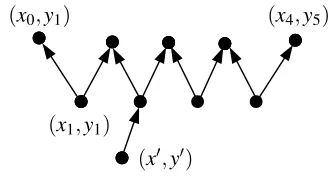
Definition 4.4(The W-configuration). Supposev≈(x,y)has in-degree at most one, and the backward path contains anevennumber of edges, terminating at vertexv0≈(x0,y0). We refer to this alternating path as aW-configuration. (SeeFigure 1.)
Any W-configuration can be written (in one of its two orientations) as a path of vertices labeled
(x0,y1),(x1,y1),(x1,y2), . . . ,(xs,ys),(xs,ys+1);
here the vertices(x1,y1), . . . ,(xs,ys)are at the “base” of the W-configuration. Note here that we have
written the path so that thex-coordinate changes, then they-coordinate, thenx, and so on. When written this way, we refer to(x0,ys+1)as theendpointsof the W-configuration.
Ifv≈(x,y)is a source node, then it defines a W-configuration with endpoints(x,y). This should not be considered a triviality or degeneracy, rather it will be the most important type of W-configuration.
(x0,y1)
(x1,y1)
(x0,y0)
(x4,y5)
4.2 The conditions onπkt∗ encoded byGt
At any timet, the future-subgraphGt gives certain necessary conditions onπin order for some putativeτ
to appear.Proposition 4.5describes a certain set of conditions that plays a key role in the analysis.
Proposition 4.5. For a witness subdag G and integers t≤T , the following condition is necessary to have G=Proj(τˆ≥Tt): For every W-configuration inGwith endpoints(x0,ys+1), we must haveπt(x0) =ys+1,
For example, ifv≈(x,y)is a source node ofG, thenπt(x) =y.
Proof. We prove this by induction ons. The base case iss=0; in this case we have a source node(x,y). Supposeπt(x)6=y. In order for ˆτT to contain some bad event containing(k∗,x,y), we must at some point
t0>t haveπt
0
(x) =y; lett0 be the minimal such time. ByProposition 3.2, we must encounter a bad event containing(k∗,x,∗)or(k∗,∗,y)at some intervening timet00<t0. If this bad event contains(k∗,x,y)
then necessarilyπt00(x) =ycontradicting minimality oft0. So there is a bad eventBcontaining either
(k∗,x,6=y)or(k∗,6=x,y), earlier than the earliest occurrence ofπ(x) =y. This eventBcorresponds to a
source node(x,6=y)or(6=x,y)in Proj(τˆ≥Tt). So(x,y)cannot also be a source node ofG.
We now prove the induction step. Consider a W-configuration with base(x1,y1), . . . ,(xs,ys), whose
endpoints are verticesv,v0labeled(x0,y1)and(xs,ys+1), respectively.
At some future timet0≥t we must encounter a bad eventBinvolving some subset of the source nodes, say thatBincludes(xi1,yi1), . . . ,(xir,yir)for 1≤r≤s. As these were necessarily source nodes
in Proj(τˆ≥Tt0), we hadπt 0
(xi1) =yi1, . . . ,π
t0(x
ir) =yir. After the swaps, these source nodes are removed
and so the updated Proj(τˆ≥Tt0+1)hasr+1 new W-configurations, whose length is all smaller thans. By inductive hypothesis, the updated permutationπt
0+1
must then satisfy
πt
0+1
(x0) =yi1,π
t0+1(x
i1) =yi2, . . . ,π
t0+1(x
ir) =ys+1.
ByProposition A.2, we may suppose without loss of generality that the resampling of the bad event
first swapsxi1, . . . ,xir in that order. Letπ
0denote the result of these swaps; there may be additional swaps
to other elements of the permutation, but we must haveπt
0+1
(xi`) =π
0(x
i`)for`=1, . . . ,r. Evidently
xi1 swapped with xi2, then xi2 swapped with xi3, and so on, until eventually xir was swapped with
x00= (πt
0
)−1ys+1. At this point, we haveπ0(x00) =yi1. Later swaps during timet
0may swapx00with some
otherx, where (x,y)∈B. Thus, at timet0+1 we either haveπt
0+1
(x00) =yi1 orπ
t0+1(x) =y
i1 where
(x,y)∈B. Recall thatπt0+1(x0) =yi−1; thus eitherx00=x0orx=x0.
In the latter case, (x0,y)∈B. Thus implies that, when we encounter the bad event Bat time t0, there is a source node labeled(x0,y)∈Proj(τˆ≥Tt0). This node(x0,y)would also occur in Proj(τˆ≥Tt). So
(x0,y1),(x1,y1), . . . ,(xs,ys+1)cannot be a W-configuration in Proj(τˆ≥Tt), although it is a W-configuration
inG.
Thus, we conclude thatx00=x0. So(πt
0
)−1ys=x00=x0or equivalentlyπt 0
(x0) =ys. This in turn
implies thatπt(x0) =ys+1. For, byProposition 3.2, otherwise we would have encountered a bad event involving(x0,∗)or(∗,ys+1); these would imply an additional in-neighbor ofvorv0, respectively, which contradicts that it is part of a W-configuration of Proj(τˆ≥Tt).
Definition 4.6(Active conditions of a witness subdag). We refer to the conditions implied by Proposi-tion 4.5as theactive conditionsof the witness subdagG. More formally, we define
Active(G) ={(x,y)|(x,y)are the end-points of aW-configuration ofG}.
We also defineAtk to be the cardinality of Active(Gt), that is, the number of active conditions of
permuta-tionπkat timet. (The subscriptkmay be omitted in context, as usual.)
Lemma 4.7. Suppose G is a witness subdag which has source nodes v1≈(x1,y1), . . . ,vr≈(xr,yr)
(plus possibly some additional source nodes). Let H =G−v1− · · · −vr. Then there is a set Z ⊆
{(x1,y1), . . . ,(xr,yr)}with the following properties:
1. There is aninjectivefunction f :Z→Active(H), with the property that(x,y)∼f((x,y))for all (x,y)∈Z .
2. |Active(H)|=|Active(G)| −(r− |Z|).
Intuitively, we are saying that every node(x,y)we are removing is either explicitly constrained in an “independent way” by some new condition in the graph H (corresponding to Z), or it is almost totally unconstrained.
Expository remark. We have recommended bearing in mind the special case when each bad event consists of a single element. In this case, we would have r=1; and the stated theorem would be that either
|Active(H)|=|Active(G)| −1; OR|Active(H)|=|Active(G)|and(x1,y1)∼(x10,y01)∈Active(H).
Proof. LetHi=G−v1− · · · −vi. We will recursively build up a setZiand functions fi:Zi→Active(Hi),
whereZi⊆ {(x1,y1), . . . ,(xi,yi)}, and which satisfy the given conditions up to stagei.
We remove the source nodevi from Hi−1. Observe that(xi,yi)∈Active(Hi−1), but (unless there is some other vertex with the same label inG),(xi,yi)6∈Active(Hi). Thus, the most obvious change
when we removeviis that we destroy the active condition(xi,yi). This may add or subtract other active
conditions as well.
We will need to updateZi−1,fi−1. Most importantly, fi−1may have mapped(xj,yj)for j<i, to an
active condition ofHi−1which is destroyed whenviis removed. In this case, we must re-map this to a
new active condition. Note that we cannot have fi−1(xj,yj) = (xi,yi)for j<i, asxi6=xjandyi6=yj.
There are now a variety of cases depending on the forward path ofviinHi−1.
1. This forward path consists of a cycle, or the forward path terminates on both sides in forward edges. This is the easiest case. Then no more active conditions ofHi−1are created or destroyed. We updateZi =Zi−1,fi = fi−1. One active condition is removed, in net, from Hi−1; hence |Active(Hi)|=|Active(Hi−1)| −1.
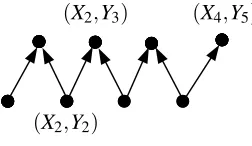
2. This forward path contains a forward edge on one side and a backward edge on the other. For example, suppose the path has the form(X1,Y1),(X1,Y2),(X2,Y2), . . . ,(Xs,Ys+1), where the vertices
case, we do not destroy any W-configurations, but we create a new W-configuration with endpoints
(Xj,Ys+1) = (xi,Ys+1).
We now updateZi=Zi−1∪ {(xi,yi)}. We define fi= fi−1plus we map(xi,yi)to the new active
condition (xi,Ys+1). In net, no active conditions were added or removed, and|Active(Hi)|=
|Active(Hi−1)|.
(X2,Y2)
(X2,Y3) (X4,Y5)
Figure 2: When we remove(X2,Y2), we create a new W-configuration with endpoints(X2,Y5).
3. This forward path was a W-configuration (X0,Y1),(X1,Y1), . . . ,(Xs,Ys),(Xs,Ys+1)with the pairs
(X1,Y1), . . . ,(Xs,Ys) on the base, and we had (xi,yi) = (Xj,Yj). This is the most complicated
situation; in this case, we destroy the original W-configuration with endpoints(X0,Ys+1)but create two new W-configurations with endpoints(X0,Yj)and(Xj,Ys+1). We updateZi=Zi−1∪ {(xi,yi)}.
We will set fi= fi−1, except for a few small changes as follows.
If(fi−1)−1(X0,Ys+1) = /0 then simply set fi(xi,yi) = (X0,Yj). Otherwise, we have fi−1(x`,y`) = (X0,Ys+1) for some ` < i; so either x` =X0 or y` =Ys+1. If it is the former, set fi(x`,y`) = (X0,Yj),fi(xi,yi) = (Xj,Ys+1). If it is the latter, set fi(x`,y`) = (Xj,Ys+1),fi(xi,yi) = (X0,Yj).
In any case, fi is updated appropriately, and in the net no active conditions are added or removed, so|Active(Hi)|=|Active(Hi−1)|.
5
The probability that the swaps are all successful
In the previous sections, we determined necessary conditions for the permutationsπkt, depending on the
graphsGk,t. In this section, we finish by computing the probability that the swapping subroutine causes
the permutations to, in fact, satisfy all such conditions.
Proposition 5.1states the key randomness condition satisfied by the swapping subroutine. The
basic intuition is as follows: supposeπ :[n]→[n] is a fixed permutation withπ(x) =y, and π0 =
Swap(π;x1, . . . ,xr). Thenπ0(x1)has a uniform distribution over[n]. Similarly,π0−1(y1)has a uniform distribution over[n]. However, the joint distribution isnotuniform—there is essentially only one degree of freedom for the two values. In general, any subset of the variablesπ0(x1), . . . ,π0(xr),π0−1(y1), . . . ,π−1(yr)
will have the uniform distribution,as long as the subset does not simultaneously containπ0(xi),π0−1(yi)
for some i∈[r].
1. 0≤s≤min(q,r).
2. q+ (r−s)≤n.
Letπ be a fixed permutation of[n]. Let x1, . . . ,xr∈[n]be distinct, and let yi=π(xi)for i=1, . . . ,r.
Defineπ0=Swap(π;x1, . . . ,xr).
Consider a list(x01,y01), . . . ,(x0q,y0q)satisfying the following properties:
3. All x0are distinct; all y0are distinct.
4. For i=1, . . . ,s we have(xi,yi)∼(x0i,y0i).
Then we have the bound:
P(π0(x01) =y10 ∧ · · · ∧π0(x0q) =y
0
q)≤
(n−r)!(n−q)!
n!(n−q−r+s)!.
Expository remark. Consider the special case when each bad event contains a single element. In that case, we only need to use this result for r=1. There are two possibilities for s; either s=0in which case this probability on the right is1−q/n (i. e., the probability thatπ0(x1)6=y01, . . . ,y0q); or s=1in which
case this probability is1/n (i. e., the probability thatπ0(x1) =y01).
Proof. Define the function
g(n,r,s,q) = (n−r)!(n−q)! n!(n−q−r+s)!.
We will prove this proposition by induction ons,r, considering a number of separate cases.
1. Supposes>0 andx1=x01. Then, in order to satisfy the desired conditions, we must swap x1 tox00=π−1(y01); this occurs with probability 1/n. The subsequentr−1 swaps starting with the
permutationπ(x1x00)must now satisfy the conditionsπ0(x02) =y02, . . . ,π0(xq) =y0q. We claim that
(xi,π(x1x00)xi)∼(x0i,y0i)fori=2, . . . ,s. Ifx006=x2, . . . ,xs, this is immediate. Otherwise, suppose
x00=xj. Ifxj =x0j, then we again still have(xj,π(x1x00)xj)∼(x0j,y0j). Ifyj=y0j, then this implies
thaty01=yj=y0j, which contradicts that they
0
j6=y
0
1.
So we apply the induction hypothesis toπ(x1x00); in the induction, we subtract one fromn,q,r,s. This gives
P(π0(x01) =y01∧ · · · ∧π(x0q) =y
0
q)≤
1
ng(n−1,r−1,s−1,q−1) =g(n,r,s,q)
as desired.
2. Similarly, supposes>0 and supposey1=y01. ByProposition A.3, we would obtain the same distribution if we executed(π0)−1=Swap(π−1;y1, . . . ,yr), so
P(π0(x01) =y01∧ · · · ∧π(x0q) =y
0
q) =P((π
0)−1(y0
1) =x
0
1∧ · · · ∧(π
0)−1(y0
q) =x
0
q).
3. Supposes=0 and there are indicesi∈[r],j∈[q]with(xi,yi)∼(x0j,y
0
j). ByProposition A.2, we
can assume without loss of generality that(x1,y1)∼(x01,y01). So, in this case, we are really in the case withs=1. This is covered by case (1) or case (2), which we have already shown. Thus, we have
P(π0(x01) =y01∧ · · · ∧π(xq0) =y
0
q)≤g(n,r,1,q) =
g(n,r,0,q)
n−q−r+1 ≤g(n,r,s,q). Here, we are using our hypothesis thatn≥q+ (r−s) =q+r.
4. Finally, supposes=0 and x1, . . . ,xr are distinct fromx01, . . . ,x0qand y1, . . . ,yqare distinct from
y01, . . . ,y0q. In this case, a necessary condition to have π0(x01) =y01, . . . ,π(xq0) =y0q is that there
are some y001, . . . ,y00r, distinct from each other and distinct fromy01, . . . ,y0q, with the property that
π0(xi) =y00i for j=1, . . . ,r. By the union bound, we have
P(π0(x01) =y01∧ · · · ∧π(x0q) =y0q)≤
∑
y00 1,...,y00r
P(π0(x1) =y001∧ · · · ∧π(xr) =y00r).
For each individual summand, we apply the induction hypothesis; the summand has probability at most g(n,r,r,q). As there are (n−q)!/(n−q−r)! possible values for y001, . . . ,y00r, the total probability is at most(n−q)!/(n−q−r)!×g(n,r,r,q) =g(n,r,s,q).
We applyProposition 5.1to upper-bound the probability that the Swapping Algorithm successfully swaps when it encounters a bad event.
Proposition 5.2. Suppose we encounter a bad event B at time t containing elements (k,x1,y1), . . .,
(k,xr,yr)from permutation k (and perhaps other elements from other permutations). Then the probability
thatπkt+1satisfies all the active conditions of its future-subgraph, conditional on all past events and all
other swappings at time t, is at most
P(πkt+1satisfiesActive(Gkt+1))≤Pk(B)
(nk−Atk+1)!
(nk−Atk)!
.
Recall that we have defined Atk=|Active(Gk,t)|and we have defined Pk(B) =( nk−r)!
nk! .
Expository remark. Consider the special case when each bad event consists of a single element. In this case, Pk(B) =1/n, and the stated theorem is now: either At+1=At, in which case the probability
thatπ satisfies its swapping condition is1/n; or At+1=At−1; in which case the probability thatπ
satisfies its swapping condition is1−At+1/n.
Proof. LetHdenote the future-subgraphGk,t+1after removing the source nodes corresponding to the pairs (x1,y1), . . . ,(xr,yr). Using the notation of Lemma 4.7, we set s=|Z|and q=Atk+1. We have
Active(H) ={(x01,y01), . . . ,(x0q,y0q)}.
For each(x,y)∈Z, we havey=πkt(x), and there is an injective function f :Z→Active(H)and
(x,y)∼f((x,y)). ByProposition A.2, we can assume without loss of generalityZ={(x1,y1), . . . ,(xs,ys)}
and f(xi,yi) = (x0i,y0i). In order to satisfy the active conditions on Gk,t+1, the swapping must cause
By Lemma 4.7, we haveAtk =Atk+1+ (r−s) =q+ (r−s). Since Atk ≤n, all the conditions of
Proposition 5.1are satisfied. Thus this probability is at most
(nk−r)!
nk!
× (nk−q)!
(nk−q−r+s)!
=(nk−r)!(nk−A
t+1
k )!
nk!(nk−Atk)!
.
We finally have all the pieces necessary to proveLemma 3.1.
Lemma3.1. Letτ be a witness tree, with nodes labeled B1, . . . ,Bs. Then
P(τ appears)≤PΩ(B1)· · ·PΩ(Bs).
Proof. The Swapping Algorithm, as we have defined it, begins by selecting the permutations uniformly at random. One may also consider fixing the permutations to some arbitrary (not random) value, and allowing the Swapping Algorithm to execute from that point onward. We refer to this asstarting at an arbitrary state of the Swapping Algorithm. We will prove the following by induction onτ0: The probability, starting at an arbitrary state of the Swapping Algorithm, that the subsequent swaps cause subtreeτ0 to appear, is at most
P(τˆT=τ0for someT ≥0)≤
∏
B∈τ0
PΩ(B)×
N
∏
k=1
nk!
(nk− |Active(Projk(τ0))|)!
. (5.1)
Whenτ0=/0, the RHS of (5.1) is equal to one so this is vacuously true.
To show the induction step, note that in order forτ0to appear, it must be that someBis resampled,
where some nodev∈τ0is labeled byB. Suppose we condition on thatvis the first such node, resampled at timet. A necessary condition to have ˆτT=τ0for someT ≥tis that eachπkt+1satisfies all the active
conditions onGk,t+1. ByProposition 5.2, this has probability at most
∏
kPk(B)
(nk−Atk+1)!
(nk−Atk)!
.
Next, if this event occurs, then subsequent resamplings must cause ˆτ≥Tt+1=τ0−v. We bound this probability using the induction hypothesis. Note that the induction hypothesis gives a bound conditional onanystarting configuration of the Swapping Algorithm, so we may multiply these probabilities to get
P(τˆT=τ0 for someT >0)
≤
∏
k
Pk(B)
(nk−Atk+1)!
(nk−Atk)!
×
∏
B∈τ0−v
PΩ(B)×
N
∏
k=1
nk!
(nk− |Active(Projk(τ0−v))|)!
=
∏
B∈τ0
PΩ(B)
∏
k
(nk−Atk+1)!
(nk−Atk)!
nk!
(nk− |Active(Projk(τ0−v))|)!
=
∏
B∈τ0
PΩ(B)
∏
k
nk!
(nk−Atk)!
asAtk+1=|Active(Projk(τ
0−v))|,
We now consider the necessary conditions to produce theentirewitness treeτ, and not just fragments
of it. First, theoriginal permutationsπk0must satisfy the active conditions of the respective witness
subdags Projk(τ). For each permutationk, this occurs with probability
(nk−A0k)!
nk!
.
Next, the subsequent sampling must be compatible withτ; by (5.1) this has probability at most
∏
B∈τ
PΩ(B)×
N
∏
k=1
nk!
(nk−A0k)!
.
Again, note that the bound in (5.1) is conditional on any starting position of the Swapping Algorithm, hence we may multiply these probabilities. In total we have
P(τˆT =τ for someT ≥0)≤
∏
k
(nk−A0k)!
nk!
×
∏
B∈τ
PΩ(B)×
N
∏
k=1
nk!
(nk−A0k)!
=
∏
B∈τ
PΩ(B).
We note a counterintuitive aspect to this proof. The natural way of proving this lemma would be to identify, for each bad eventB∈τ, some necessary event occurring with probability at mostPΩ(B).
This is the general strategy in Moser & Tardos [31] and related constructive LLL variants such as [18], [1], [20]. This isnotthe proof we employ here; there is an additional factor of(nk−A0k)!/n! which is
present for the original permutation and is gradually “discharged” as active conditions disappear from the future-subgraphs.
6
The constructive LLL for permutations
Now that we have proved the Witness Tree Lemma, the remainder of the analysis is essentially the same as for the Moser–Tardos algorithm [31]. Using arguments and proofs from [31] with our key lemma, we can now easily show our key theorem:
Theorem 6.1. Suppose some function x:B→(0,1)satisfies, for every B∈B, the condition PΩ(B)≤x(B)
∏
B0∼B
B06=B
(1−x(B0)).
Then the Swapping Algorithm terminates with probability one. The expected number of iterations in which we resample B is at most x(B)/(1−x(B)).
In the “symmetric” case, this gives us the well-known LLL criterion:
Corollary 6.2. Suppose each bad event B∈Bhas probability at most p, and is dependent with at most d bad events. Then ifep(d+1)≤1, the Swapping Algorithm terminates with probability one; the expected number of resamplings of each bad event is O(1).
6.1 Lopsidependence
As in [31], it is possible to slightly restrict the notion of dependence. We can redefine the relation∼on bad events by settingB∼B0iff
1. B=B0,or
2. there is some(k,x,y)∈B,(k,x0,y0)∈B0with eitherx=x0,y6=y0orx6=x0,y=y0.
In particular, bad events which share the same triple(k,x,y), arenotcaused to be dependent.
Proving that the Swapping Algorithm still works in this setting requires only a slight change in our definition of Projk(τ). Now, the treeτ may have multiple copies of any given triple(k,x,y) on a
single level. When this occurs, we create the corresponding nodesv≈(x,y)∈Projk(τ); edges are added
between such nodes in an arbitrary (but consistent) way. The remainder of the proof remains as before.
6.2 LLL for injective functions
The analysis of [28] considers a slightly more general setting for the LLL, in which we select random
injections fk:[mk]→[nk], wheremk≤nk. In fact, our Swapping Algorithm can be extended to this case.
We simply define a permutationπkon[nk], where the entriesπk(mk+1), . . . ,πk(nk)are “dummies” which
do not participate in any bad events. The LLL criterion for the extended permutationπk is exactly the
same as the corresponding LLL criterion for the injection fk. Because all of the dummy entries have
the same behavior, it is not necessary for the Swapping Algorithm to keep track of the dummy entries exactly; they are needed only for the analysis.
6.3 Comparison with the approaches of Achlioptas & Iliopoulos and Harvey & Vondrák
Achlioptas & Iliopoulos [1] and Harvey & Vondrák [20] gave generic frameworks for analyzing variants of the Moser–Tardos algorithm, applicable to different types of combinatorial configurations. These frameworks can include vertex colorings, permutations, Hamiltonian cycles of graphs, spanning trees, matchings, and other settings. For the case of permutations, both of these frameworks give a version of the Swapping Algorithm and show that it terminates under the same conditions as we do, which in turn are the same conditions as the LLL (Theorem 1.1).
The key difference between our approach and [1,20] is that they enumerate the entire history of all resamplings to the permutations. In contrast, our proof is based on the Witness Tree Lemma; this is a much more succinct structure that ignores most of the resamplings, and only enumerates the few resamplings that are necessary to justify a single item in the execution log. Their proofs are much simpler than ours; a major part of the complexity of our proof lies in the need to argue that the bad events which were ignored by the witness tree do not affect the probabilities. (The ignored bad eventsdointeract with the variables we need to track for the witness tree, but do so in a “neutral” way.)
execution of the Swapping Algorithm. The proof strategy of Moser & Tardos is to take a union bound over all witness trees that correspond to this event. In this case, we show a probability bound which is proportional to the total weight of all such witness trees. This can be a relatively small number as only the witness trees connected toE are relevant. Our analysis, which is also based on witness trees, is able to show similar types of bounds.
However, the analysis of Achlioptas & Iliopoulos and Harvey & Vondrák is not based on witness trees, but the much larger set offull execution logs. The number of possible execution logs can be exponentially larger than the number of witness trees. It is very inefficient to take a union bound over all such logs. Hence, Achlioptas & Iliopoulos and Harvey & Vondrák give bounds which are exponentially weaker (in a certain technical sense) than the ones we provide.
Many properties of the Swapping Algorithm depend on the fine degree of control provided by the Witness Tree Lemma, and it seems difficult to obtain them from the alternate LLLL approaches. We list a few of these properties here.
The LLL criterion without slack.As a simple example of the problems caused by taking a union bound over execution logs, suppose that we satisfy the LLL criterion without slack, say ep(d+1) =1; here, as usual, pandd are bounds, respectively on the probability of any bad event and the degree of any bad event in the dependency graph. In this case, we show that the expected time for our Swapping Algorithm to terminate isO(m). In contrast, in Achlioptas & Iliopoulos or Harvey & Vondrák, they require satisfying the LLL criterion with slack ep(1+ε)(d+1) =1, and achieve a termination time of
O(m/ε). They require this slack term in order to damp the exponential growth in the number of execution
logs. (Harvey & Vondrák show that if the symmetric LLL criterion is satisfied without slack, then the Shearer criterion [34] is satisfied with slackε=Ω(1/m). Thus, they would achieve a running time of
O(m2)without slack.)
Arbitrary choice of which bad event to resample. The Swapping Algorithm as we have stated it is actually underdetermined, in that the choice of which bad event to resample is arbitrary. In contrast, in both Achlioptas & Iliopoulos and Harvey & Vondrák, there is a fixed priority on the bad events. (Kolmogorov [26] has shown that this restriction can be removed in certain special cases of the Achlioptas & Iliopoulos setting, including for random permutations and matchings.) This freedom can be quite useful. For example, inSection 7we consider a parallel implementation of our Swapping Algorithm. We will select which bad events to resample in a quite complicated and randomized way. However, the correctness of the parallel algorithm will follow from the fact that it simulates some serial implementation of the Swapping Algorithm.
The Moser–Tardos distribution.The Witness Tree Lemma allows us to analyze the so-called “Moser– Tardos (MT) distribution,” first discussed by [16]. The LLL and its algorithms ensure that bad events
Bcannot possibly occur. In other words, we know that the configuration produced by the LLL has the property that noB∈Bis true. In many applications of the LLL, we may wish to know more about such configurations, other than they exist.
We give two examples where this useful for the ordinary, variable-based LLL. First, suppose that we have some weights for the values of our variables, and we define the objective function on a solution
∑iw(Xi); in this case, if we are able to estimate the probability that a variableXitakes on value jin the
perhaps exponentially large. In this case, the Moser–Tardos algorithm cannot test them all. However, we may still be able to ignore a subset of the bad events, and argue that the probability that they are true at the end of the Moser–Tardos algorithm is small even though they were never checked.
The Witness Tree Lemma gives us an extremely powerful result concerning this MT distribution, which carries over to the Swapping Algorithm.
Proposition 6.3. Let E ≡πk1(x1) =y1∧ · · · ∧πkr(xr) =yr. Then the probability that E is true in the
output of the Swapping Algorithm, is at most
PΩ(E)
∏
B∼E
(1−x(B))−1.
Proof. See [16] for the proof of this for the ordinary MT algorithm; the extension to the Swapping Algorithm is straightforward.
Bounds on the depth of the resampling process.One key requirement for parallel variants of the Moser– Tardos algorithm appears to be that the resampling process has logarithmic depth. This is equivalent to showing that there are no deep witness trees. This follows easily from the Witness Tree Lemma, along the same lines as in the original paper of Moser & Tardos, but appears to be very difficult in the other LLLL frameworks.
Partial resampling.In [18], a partial resampling variant of the Moser–Tardos algorithm was developed. In this variant, one only resamples a small, random subset of the variables (or, in our case, permutation elements) which determine a bad event. To analyze this variant, [18] developed an alternate type of witness tree, which only records the variables which were actually resampled. Ignoring the other variables can drastically prune the space of witness trees. Again, this does not seem to be possible in other LLLL frameworks in which thefullexecution log must be recorded. We will see an example of this in
Theorem 8.2; we do not know of any way to show results such asTheorem 8.2using the frameworks of
either Achlioptas & Iliopoulos or Harvey & Vondrák.
7
A parallel version of the Swapping Algorithm
The Moser–Tardos resampling algorithm for the ordinary LLL can be transformed into anRNCalgorithm by allowing a slight slack in the LLL’s sufficient condition [31]. The basic idea is that in every round, we select amaximal independent set (MIS)of bad events to resample. Using the known distributed/parallel algorithms for MIS, this can be done inRNC; the number of resampling rounds is then shown to be logarithmic w. h. p. (“with high probability”), in [31].
In this section, we will describe a parallel algorithm for the Swapping Algorithm, which runs along the same lines. However, everything is more complicated than in the case of the ordinary LLL. In the Moser–Tardos algorithm, events which are not connected to each other cannot affect each other in any way. For the permutation LLL, such events can interfere with each other, but do so rarely. Consider the following example. Suppose that at some point we have two active bad events, “πk(1) =1” and
“πk(2) =2,” and so we decide to resample them simultaneously (since they are not connected to each
swap 1 with 2; this automatically fixes the second bad event as well. The sequential algorithm, in this case, would only swap a single element. The parallel algorithm should likewisenotperform a second swap for the second bad event, or else it would be oversampling. Avoiding this type of conflict is quite tricky.
Letn=n1+· · ·+nN; since the output of the algorithm will be the contents of the permutations
π1, . . . ,πk, this algorithm should be measured in terms ofn, and we must show that this algorithm runs in
polylog(n)time. Our algorithm will require that|B|, the total number of bad events, is polynomial inn, and that every elementB∈Bhas size|B| ≤polylog(n); these conditions hold for many cases.
We describe the following Parallel Swapping Algorithm:
1. In parallel, generate the permutationsπ1, . . . ,πN uniformly at random.
2. We proceed through a series ofroundswhile there is some true bad event. In roundi(i=1,2, . . . ,) do the following:
3. LetVi,1⊆Bdenote the set of bad events which are currently true at the beginning of roundi. We will attempt to fix the bad events inVi,1through a series ofsubrounds. This may introduce new bad events, but we will not fix any newly created bad events until roundi+1.
Repeat the following process for j=1,2, . . .as long asVi,j6=/0:
4. LetIi,j be an MIS ofVi,j.
5. For each bad eventB={(k1,x1,y1), . . . ,(kr,xr,yr)} ∈Ii,j, choose the swaps
correspond-ing toB. We select eachz`∈[nk`], which is the element to be swapped withπk`(x`) according to procedure Swap.Do not perform the indicated swaps at this time though!
We refer to(k1,x1), . . . ,(kr,xr)as the swap-sources ofBand the(k1,z1),. . .,(kr,zr)as
the swap-mates ofB.
6. Select a random orderingρi,j of the elements ofIi,j. Consider the graphGi,j whose
vertices correspond to elements of Ii,j, with an edge on (B,B0) if ρi,j(B)<ρi,j(B0)
and one of the swap-mates of B is a swap-source of B0. Generate Ii0,j ⊆Ii,j as the
lexicographically first MIS(LFMIS) of the resulting graphGi,j, with respect to vertex
orderingρi,j.
7. For each permutationπk, enumerate all the transpositions(x z)corresponding to elements
ofIi0,j, arranged in order ofρi,j. Say these transpositions are, in order(x1,z1), . . .(x`,z`).
Compute, in parallel for allπk, the compositionπk0=πk(x1z1). . .(x`z`).
8. UpdateVi,j+1fromVi,j by removing all elements which are either no longer true for the
current permutation,orare connected via∼to some element ofIi0,j.
Most steps of this algorithm can be implemented using standard parallel methods. For example, step (1) can be performed simply by having each element of[nk]choose a random real and then executing a
parallel sort. The independent setIi,jcan be found in time in polylogarithmic time using [6,29].
The difficult step to parallelize is in selecting the LFMISIi0,j. In general, the problem of finding the LFMIS isP-complete [11], hence we do not expect a generic parallel algorithm for this. However, what saves us it that the orderingρi,jand the graphGi,jare constructed in a highly random fashion.
1. LetH1be the directed graph obtained by orienting all edges ofGi,jin the direction ofρi,j. Repeat
the following fors=1,2, . . . ,:
2. IfHs=/0 terminate.
3. Find all source nodes ofHs. Add these toIi0,j.
4. ConstructHs+1by removing all source nodes and all successors of source nodes fromHs.
The output of this algorithm is the LFMISIi0,j. Each step can be implemented in parallel timeO(logn). The number of iterations of this algorithm is at most the length of the longest directed path inG0i,j. So it suffices it show that, w. h. p., all directed paths inG0i,j have length polylog(n).
Proposition 7.1. Let I⊆B be an an arbitrary independent set of true bad events, and suppose all elements ofBhave size≤M. Let G=Gi,j be the graph constructed in Step (6) of the Parallel Swapping
Algorithm.
Then w. h. p., every directed path in G has length O(M+logn).
Proof. One of the main ideas below is to show that for thetypical B1, . . . ,B`∈I, where`=5(M+logn),
the probability thatB1, . . . ,B`form a directed path is small. Suppose we selectB1, . . . ,B`∈Iuniformly
at random without replacement. Let us analyze how these could form a directed path inG. (We may assume|I|> `or otherwise the result holds trivially.)
First, it must be the case thatρ(B1)<ρ(B2)<· · ·<ρ(B`). This occurs with probability 1/`!.
Next, the swap-mates ofBsmust overlap the swap-sources ofBs+1, fors=1, . . . , `−1. Now,Bs
hasO(M)swap-mates; each such swap-mate can overlap with at most one element ofI, sinceI is an independent set. Conditional on having chosenB1, . . . ,Bs, there remain|I| −schoices forBs+1. This gives that the probability of havingBswith an edge toBs+1, conditional on the previous events, is at most
M/(|I| −s). (The fact that swap-mates are chosen randomly does not give too much of an advantage here.)
Putting this all together, the total probability that there is a directed path onB1, . . . ,B`is
P(directed pathB1, . . . ,B`)≤
M`−1(|I| −`)!
(|I| −1)!`! .
The above was for a randomB1, . . . ,B`, so the probability that there issomesuch length-`path is at
most
P(some directed path)≤ |I|!
(|I| −`)!×
Ml−1(|I| −`)!
(|I| −1)!`! =|I| ×
Ml−1
`! ≤n×
M`−1 (`/e)` ≤n
−Ω(1),
since`=5(M+logn).
Proposition 7.2. Suppose|B| ≤poly(n)and all elements B∈B have size|B| ≤M. Then w. h. p. we haveVi,j=/0for some j=O(Mlog2n).
Observe that if there is noB0∈Isuch thatρ(B0)<ρ(B)and such that a swap-mate ofB0overlaps with
a swap-source ofB, thenB∈I0(this is not a necessary condition). We will analyze the orderingρusing
the standard trick, in which each elementB∈Ichooses a rankW(B)∼Uniform[0,1], independently and identically. The orderingρis then formed by sorting in increasing ordering ofW. In this way, we are
able to avoid the dependencies induced by the rankings. For the moment, suppose that the rankW(B)is
fixedat some real valuew. We will then count how manyB0∈I satisfyW(B0)<wand a swap-mate ofB0
overlaps a swap-source ofB.
So consider some swap-sourcesofBin permutationk, and consider someB0j∈Iwhich hasr0jother elements in permutationk. For`=1, . . . ,r0j, there arenk−`+1 possible choices for the`thswap-mate
fromB0j, and hence the total expected number of swap-mates ofB0which overlapsis at most
E[# swap-mates ofB0joverlappings]≤
r0j
∑
`=1 1
nk−`+1
≤
Z r0
j+1
`=1
d` nk−`+1
=ln nk
nk−r0j
!
.
Next, sum over allB0j ∈I. SinceI is an independent set, we must have∑r0j ≤nk−1. Thus, by
concavity of the ln function,
E[# swap-mates of someB0joverlappings]≤
∑
j
ln nk
nk−r0j
!
≤ln nk
nk−∑jr0j
!
≤lnnk≤lnn.
Summing over all swap-sources ofB, the total probability that there is someB0withρ(B0)≤Band for
which a swap-mate overlaps a swap-source ofB, is at mostw|B|lnn≤wMlnn. By Markov’s inequality,
P(B0∈I0|W(B) =w)≥1−wMlnn.
Integrating overwgives
P(B0∈I0)≥1− 1 2Mlnn.
Now, using this fact, we show thatVi,jis decreasing quickly in size. For, supposeB∈Vi,j. SoB∼B0
for someB0∈Ii,j, asIi,jis a maximal independent set (possiblyB=B0). We will removeBfromVi,j+1if
B0∈Ii0,j, which occurs with probability at least 1−1/(2Mlnn). AsBwas an arbitrary element ofVi,j,
this shows that
E|Vi,j+1|
Vi,j
≤1− 1 2Mlnn
|Vi,j|.
For j=Ω(Mlog2n), this implies that
E |Vi,j|
≤1− 1 2Mlnn
Ω(Mlog2n)
|Vi,1| ≤n−Ω(1).
This in turn implies thatVi,j=/0 with high probability, for j=Ω(Mlog2n).