Partially Dynamic Algorithms for Distributed
Shortest Paths and their Experimental Evaluation
Serafino Cicerone, Gianlorenzo D’Angelo, Gabriele Di Stefano, Daniele Frigioni, Alberto Petricola
Dipartimento di Ingegneria Elettrica e dell’Informazione Universit`a dell’Aquila, I-67040 Monteluco di Roio, L’Aquila, Italy E-mail:{cicerone,gdangelo,gabriele,frigioni,petricol}@ing.univaq.it
Abstract— In this paper, we study the dynamic version of the distributed all-pairs shortest paths problem. Most of the solutions given in the literature for this problem, either (i) work under the assumption that before dealing with an edge operation, the algorithm for the previous operation has to be terminated, that is, they are not able to update shortest paths concurrently, or (ii) concurrently update shortest paths, but their convergence can be very slow (possibly infinite). In this paper we propose a partially dynamic algorithm that overcomes most of these limitations. In particular, it is able to concurrently update shortest paths and in many cases its convergence is quite fast. These properties are highlighted by an experimental study whose aim is to show the effectiveness of the proposed algorithms also in the practical case.
Index Terms— Distributed networks, dynamic algorithms, shortest paths, routing, experimental evaluation, network simulation environment
I. INTRODUCTION
We consider the distributed all-pairs shortest paths problem in a network whose topology dynamically changes over the time, in the sense that communication links can change status during the lifetime of the network. This problem arises naturally in practical applications. For instance, the OSPF protocol, widely used in the Internet (e.g., see [2]), basically updates shortest paths after a network change by distributing the network topology to all processors and using centralized Dijkstra’s algorithm for shortest paths on every node.
If the topology of a network is represented as a weighted graph, where nodes represent processors, edges represent links between processors, and edge weights represent costs of communication among processors, then the typical update operations on a dynamic network can be modelled as insertions and deletions of edges and edge weight changes. When arbitrary sequences of the above operations are allowed, we refer to the fully dynamic problem; if only insert and weight decrease (delete and weight increase) operations are allowed, then we refer
This paper is based on “Partially Dynamic Concurrent Update of Dis-tributed Shortest Paths” by Gianlorenzo D’Angelo, Serafino Cicerone, Gabriele Di Stefano, Daniele Frigioni, which appeared in the Proceed-ings of the IEEE International Conference on Computing: Theory and Applications, March 2007, Kolkata, India. c°2007 IEEE [1].
Work partially supported by the Future and Emerging Technologies Unit of EC (IST priority, 6th FP), under contract no. FP6-021235-2 (project ARRIVAL).
to the incremental (decremental) problem. Incremental and decremental problems are usually called partially dynamic.
In many crucial routing applications the worst case complexity of the adopted protocols is never better than recomputing the shortest paths from scratch after each change to the network. Therefore, it is important to find efficient dynamic distributed algorithms for shortest paths, since the recomputation from scratch could result very expensive in practice. The efficiency of a distributed algorithm is evaluated in terms of message and space complexity (e.g., see [3]). The message complexity is the total number of messages sent over the edges. The space complexity is the space usage per node.
In this paper we consider a dynamic network in which a change can occur while another change is under pro-cessing. A processor v could be affected by both these changes. As a consequence, v could be involved in the concurrent executions related to both the changes.
Previous works. Given a weighted graphGwithnnodes and m edges, many solutions have been proposed in the literature to find and update shortest paths in the sequential case on graphs with non-negative real edge weights. The state of the art is that no efficient fully dynamic solution is known for general graphs that is faster than recomputing single-source shortest paths from scratch after each update. Actually, only output bounded fully dynamic solutions are known on general graphs [4], [5]. In the case of all-pairs shortest paths an efficient fully dynamic solution has been proposed in [6] that works in
O(n2log3n)amortized time per update.
drawback of the Bellman-Ford algorithm and its variations that is avoided in many protocols by broadcasting the whole topology of the network to all nodes [2], [16]. Furthermore, if the network is asynchronous and static, the message complexity of the Bellman-Ford method can be exponential in the size of the network (see, [17]). In [9] Humblet proposes a variation of the Bellman-Ford algorithm, that has the same message and space complexity, and, under certain conditions, avoids the looping phenomenon thus converging in a finite number of steps.
In [10], an efficient incremental solution has been pro-posed for the distributed all-pairs shortest paths problem, requiringO(nlog(nW))amortized number of messages, and the difficulty of dealing with edge deletions has been addressed. Here, W is the largest positive integer edge weight. In [7], a general technique is proposed that allows to update the all-pairs shortest paths in a distributed network inΘ(n)amortized number of messages, by using
O(n2)space per node. In [12], algorithms are given for
both finding and updating shortest paths distributively. In particular, the authors propose a distributed algorithm for finding single source shortest paths (all pairs shortest paths) of a network with positive real edge weights requiring Θ(n2) (O(n3)) messages and O(n) space per
node. Furthermore, they propose a distributed incremental algorithm requiringO(n2)messages for updating all-pairs
shortest paths. Finally, they give fully dynamic algorithms for single-source (all-pairs) shortest paths that work in
O(n2) (O(n3)) messages, and show that, in the worst
case, updating shortest paths is as difficult as computing shortest paths.
In [8] a solution for the fully dynamic distributed all-pairs shortest paths problem is presented whose message complexity is evaluated in terms of output complexity (see [4], [5]). Output complexity allows to evaluate the cost of dynamic algorithms in terms of the intrinsic cost of the problem on hand, i.e., in terms of the number of updates to the output information of the problem that are needed after any input change. The algorithm in [8] is able to update only the distances and the shortest paths that actually change after an edge modification σ. It requires in the worst case O(maxdeg·∆σ) messages per edge update operation. The space complexity isO(n)
per node. Here, maxdeg is the maximum degree of the nodes in the network and ∆σ is the number of pairs of nodes affected by σ. On one hand, if ∆σ = o(n2),
then these bounds compare favorably with respect to those in [12]. On the other hand, the algorithm is not robust, in fact for weight increase operations it works in three phases and requires that a phase is terminated before the execution of the subsequent one, while in the case of weight decrease operations it works under the assumption that before dealing with an edge operation, the algorithm for the previous operation has to be terminated.
Summarizing, we can conclude that most of the algo-rithms of the literature for the dynamic distributed shortest paths problem fall in one of the following categories:
• algorithms which are not able to concurrently update shortest paths when multiple edge changes occur in the network, as those in [7], [8], [10], [12]. In partic-ular, algorithms that work under the assumption that before dealing with an edge operation, the algorithm for the previous operation has to be terminated. This is a limitation in real networks, where changes can occur in an unpredictable way;
• algorithms which are able to concurrently update shortest paths as those in [9], [13], but (i) either they suffer of the looping and count-to-infinity phe-nomena, or (ii) their convergence can be very slow in the case of weight increase operations (possibly infinite).
Results of the paper. In this paper we provide partially dynamic solutions that do not belong to any of the pre-vious categories. In particular, our algorithms are able to concurrently update shortest paths, they avoid the looping and count-to-infinity phenomena and their convergence is fast in the case of weight increase operations. The details of this contribution can be summarized as follows:
1) We propose a new decremental algorithm that is robust since it works in one phase (thus avoid-ing the main drawback of [8]). Furthermore, it is able to concurrently update shortest paths in the case of multiple weight increase/delete oper-ations. The algorithm requires O(maxdeg · ∆2) messages andO(maxdeg·n)space per node. Here,
∆ is the number of nodes affected by a set of weight increase/delete operations.
2) We propose an extension of the incremental algo-rithm in [8] for weight decrease/insert operations that works also in the concurrent case, within the same bounds of [8], that is O(maxdeg· ∆)
messages per operation and O(n)space per node. Here, ∆ is the number of nodes affected by a set of weight decrease/insert operations. This is only a factor maxdeg far from the optimal incremental solution.
3) We propose an experimental study whose aim is to highlight the merits of the proposed algorithms also from a practical point of view. In detail, we experimentally show that our incremental algorithm sends a number of messages that is 10%–15% less than Bellman-Ford.
count-to-infinity phenomena in some classical cases where BF.1 and BF.2 do.
Structure of the paper. The paper is organized as follows. In Section II we introduce the notation and the computation model used throughout the paper. In Sections III and IV we describe the algorithms for weight increase and weight decrease operations, respectively, and show their complexity in terms of number of messages. In Section V we describe the experiments performed to check the effectiveness of our algorithms in the practical case. Finally, in Section VI we provide some concluding remarks and future research directions.
II. PRELIMINARIES
We consider a network made of processors linked through communication channels. Each processor can send messages only to its neighbors. Messages are de-livered to their destination within a finite delay but they might be delivered out of order. We consider an asyn-chronous system, that is, a sender of a message does not wait for the receiver to be ready to receive the message. There is no shared memory, that is, each processor has its own storage system and the other processors cannot access it.
We represent the network by an undirected weighted graphG= (V, E, w), where V is a finite set ofnnodes, one for each processor; E is a finite set of m edges, one for each communication channel; andw is a weight functionw:E→R+. An edgee∈Ethat links the pair
of nodes u, v∈V is represented with u→v. If v ∈V,
N(v) denotes the set of neighbors of v and deg(v) the degree of v.
We define the weight of a path P as the sum of the weights of the edges inP. The distance between nodesu
andvis the weight of a shortest path fromutov, and is denoted as d(u, v). Givenu, v ∈V, the via fromutov is the set of neighbors ofuthat belong to a shortest path from utov. Formally,
via(u, v)≡ {z∈N(u)|d(u, v) =w(u, z) +d(z, v)}
Complexity measures. Given a weighted undirected graph G, a set of k weight changes σ1, σ2, ..., σk and a
sources, we denote asδσi,sthe set of nodes that change the distance tosas a consequence ofσi. Ifv∈ ∪
s∈Vδσi,s
we say thatvis affected byσi. The total number of times that nodes ofGare affected by thekweight changes is at
most∆ = Pk i=1
P
s∈V
|δσi,s|. We give the complexity bounds
of our algorithms as a function of ∆.
Asynchronous model. Given an asynchronous system, the model summarized below is based on that proposed in [3]. The state of a processor v is the content of the data structure at node v. The network state is the set of states of all the processors in the network plus the network topology. An event is the reception of a message by a processor or a change to the network state. When a processor psends a messagem to a processorq, mis
stored in a buffer in q. When q readsm from its buffer and processes it, the event “reception of m” occurs.
An execution is an alternate sequence (possibly infinite) of network states and events. A non negative real number is associated to each event, the time at which that event occurs. The time is a global parameter and is not acces-sible to the processors of the network. The times must be non decreasing and must increase without bound if the execution is infinite. Events are ordered according to the times at which they occur. Several events can happen at the same time as long as they do not occur at the same processor. This implies that the times related to a single processor are strictly increasing.
Concurrent executions. In this paper we consider a dynamic network in which a change can occur while another change is under processing. A processor v could be affected by both these changes. As a consequence, v could be involved in the executions related to both the changes. Hence, according to the asynchronous model we need to define the notion of concurrent executions as follows.
Let us consider an algorithmAthat maintains shortest paths on G after a weight change operation. Given two operations σi andσj we denote as:
• ti and tj the times at which σi and σj occur respectively.
• Ai (Aj) the execution ofA related toσi (σj).
• tAi the time whenAi terminates.
If ti ≤tj andtAi ≥tj, thenAi andAj are concurrent, otherwise they are sequential.
III. DECREMENTAL ALGORITHM
In this Section we describe our new decremental so-lution for the concurrent update of distributed all-pairs shortest paths in the case of multiple operations. We con-sider the algorithm to handle weight increase operations, since the extension to delete operations is straightforward (deleting an edge(x, y)is equivalent to increasew(x, y) to+∞).
Given the input graph G = (V, E, w), we suppose that k weight increase operations σ1, σ2, ..., σk are
per-formed on edges (xi, yi)∈E,i∈ {1,2, ..., k}, at times
t1, t2, ..., tk, respectively. The operation σi increases the
weight w(xi, yi)by a quantity ²i >0,i ∈ {1,2, ..., k}. Without loss of generality, we assume that t1 ≤ t2 ≤ ...≤tk. We denote asG0 the graph aftertk, as d0()and
via0()the distance and the via overG0, respectively.
Data structures. A node knows the identity of each node of the graph, the identity of all its neighbors and the weight of the edges incident to it. The information on the shortest paths in Gare stored in a data structure called routing table RTdistributed over all nodes. Each nodev maintains its own routing table RTv[·]; this table has one entryRTv[s]for eachs∈V. The entryRTv[s]consists of two fields:
• RTv[s].via= {vi ∈ N(v) | RTv[s].d= w(v, vi) +
RTvi[s].d}that stores the estimated via from vtos. For sake of simplicity, we write d[v, s] and via[v, s]
instead of RTv[s].dandRTv[s].via, respectively.
The values stored in the routing table of each node change over the time during the execution of the update algorithms. Hence, we denote as dt[v, s] and viat[v, s]
the value of the data structures at timet; we simply write
d[v, s]andvia[v, s]when time is clear by the context. Algorithm. Before the decremental algorithm starts, we assume that dt[v, s] and viat[v, s] are correct, for each
v, s∈V and for eacht < t1.
The decremental algorithm starts at each ti, i ∈ {1,2, ..., k}. For instance, the weight increase operation
σi represents an event that is detected only by nodes xi andyi; as a consequence:
• xisends the message increase(xi, s,dti[xi, s])toyi, for each s∈V;
• yisends the message increase(yi, s,dti[yi, s])toxi, for each s∈V.
When, at a certain time t, node v receives the message increase(u, s,d˜t[u, s]), ˜t < t, by a generic node u, v
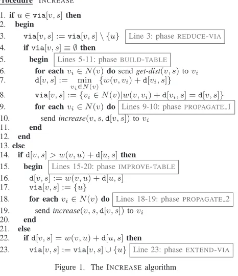
executes procedure INCREASE (see Figure 1), which is designed to updateRTv[s], if necessary. To this aim,vmay need to know the estimated distances of its neighbors from
s, that is, dt[vi, s] for each vi ∈ N(v). Hence, v sends messages get-dist(v, s); when vi receives such message, it performs procedure DIST (see Figure 2).
Event: nodevreceives the message increase(u, s,d[u, s])byu
Procedure INCREASE
1. ifu∈via[v, s]then
2. begin
3. via[v, s] :=via[v, s]\ {u} Line 3: phaseREDUCE-VIA
4. ifvia[v, s]≡ ∅then
5. begin Lines 5-11: phaseBUILD-TABLE
6. for eachvi∈N(v)do send get-dist(v, s)tovi 7. d[v, s] := min
vi∈N(v)
{w(v, vi) +d[vi, s]}
8. via[v, s] :={vi∈N(v)|w(v, vi) +d[vi, s] =d[v, s]} 9. for eachvi∈N(v)do Lines 9-10: phasePROPAGATE 1 10. send increase(v, s,d[v, s])tovi
11. end
12. end
13. else
14. ifd[v, s]> w(v, u) +d[u, s]then
15. begin Lines 15-20: phaseIMPROVE-TABLE
16. d[v, s] :=w(v, u) +d[u, s] 17. via[v, s] :={u}
18. for eachvi∈N(v)do Lines 18-19: phasePROPAGATE2 19. send increase(v, s,d[v, s])tovi
20. end
21. else
22. ifd[v, s] =w(v, u) +d[u, s]then
23. via[v, s] :=via[v, s]∪ {u} Line 23: phaseEXTEND-VIA
Figure 1. The INCREASEalgorithm
Notice that, in our model, multiple increase messages received by a node are stored and processed in an ar-bitrary order, while each message get-dist is processed immediately.
Event: nodevreceives the message get-dist(u, s)byu
Procedure DIST
1. if(via[v, s]≡ {u})or(v is performing phaseBUILD-TABLE or phaseIMPROVE-TABLEof procedure INCREASE with respect to source s)
2. then send+∞tou
3. else sendd[v, s]tou
Figure 2. Procedure DISTperformed by a nodevwhen it receives a get-dist message
Now we provide an informal description of the al-gorithm. The purpose of this description is to give an intuition of both the behavior and correctness of the algo-rithm (the formal correctness proof is given in [18]). The description is focused on the execution of the algorithm by a generic node v with respect to a source s, and uses the scenario for node v depicted in Figure 3 as a representative case.
v2
v3
v u3
u1
v4
v5
v1
u4
u2
via(v2, s) via(v, s)
via(v1, s)
Figure 3. A representative scenario
In such a figure nodes are colored white, gray and black. These colors are assigned according to the following definitions.
• a node v is white with respect to s if v does not change both its distance and its via tos. Formally:
d(v, s) =d0(v, s) and via(v, s)≡via0(v, s).
• a nodevis gray with respect tosifvdoes not change its distance froms, but it changes its via to s. For-mally:d(v, s) =d0(v, s), and via(v, s)6≡via0(v, s). Notice that, in this case, via(v, s))via0(v, s). • a nodev is black with respect tosif v changes its
distance froms. Formally:d(v, s)6=d0(v, s). Notice
that, in this case,d(v, s)< d0(v, s).
The following properties trivially hold:
P1: Ifvis gray or black with respect tos, then there existsu∈via(v, s)which is black with respect to s. If v is black with respect to s, then all nodes in via(v, s)are black with respect tos. P2: If v is white or gray with respect to s, then,
each node z such that v ∈ via(z, s) is white with respect tos.
are black. As a consequence, v surely receives mes-sages increase(ui, s,d[ui, s]), 1 ≤ i ≤ 3, in some order. This implies thatv performs three times procedure INCREASE. The first two executions simply perform phase
REDUCE-VIA, while the third one performsREDUCE-VIA
and BUILD-TABLE.
Let us suppose that the third execution is related tou3.
During the execution of BUILD-TABLE, nodev sends the message get-dist(v, s)to each nodevi∈N(v)\{u3}. We
assume that this message is received by vi at timet˜1,i.
In this phase, let us assume that the following conditions hold for nodes v1 andv3, respectively:
(a) via˜t1,1[v1, s]≡ {v}
(b) at time t˜1,3, node v3 is performing either BUILD-TABLE or IMPROVE-TABLE phases of pro-cedure INCREASEwith respect to source s According to these conditions and to test at line 1 of procedure DIST, nodesv3 andv1 send +∞ tov.
By using the collected information, v performs the instructions d[v, s] := min
vi∈N(v)
{w(v, vi) + d[vi, s]} and
via[v, s] := {vi ∈N(v)| w(v, vi) +d[vi, s] =d[v, s]}. Let us assume that now via˜t2[v, s] ={v2}. Notice that,
since v has received partial information, the content of
RTv[s]at timet˜2could be not correct. Now, two relevant
observations have to be remarked:
(i) since nodes v1 and v3 sent +∞tov, then v does
not consider such nodes as possible new elements of
via; this is done to prevent the looping and count-to-infinity phenomena.
(ii) in the subsequent Items 1 and 2 we show that nodes
v1 andv3 will eventually sendd[v1, s]andd[v3, s]
tov.
The BUILD-TABLE phase of v is completed by the
PROPAGATE 1 phase. In this phasev broadcast toN(v)
the message increase(v, s,d˜t2[v, s]); it may seem useless
to send the message to nodesui,1≤i≤3, (the old via of v) and to nodev2 (the new via ofv). The former will
be explained later (last paragraph of Item 1), while the latter is due to the fact that v∈via(v2, s), and hencev2
has to perform the REDUCE-VIAphase.
Let us now analyze what happens to the nodesv1, v3, v4
andv5.
1. nodev1receives message increase(v, s,dt˜2[v, s])at
time ˜t3 > ˜t2, and it executes INCREASE. Since
via˜t1,1[v1, s] ≡ viat˜3[v1, s] ≡ {v}, v1 performs
the BUILD-TABLE phase. At the end of this phase, at time˜t4>˜t3,v1updatesRTv1[s]. Now, two major
cases may occur:
• v is invia˜t4[v1, s];
• vis not inviat˜4[v1, s]. This means thatv1now
uses a new via tos.
In both cases, at the end of theBUILD-TABLEphase,
v1 broadcast the message increase(v1, s,d˜t4[v1, s])
to N(v1), and hence to v also (with reference to
Item (ii) above).
In the first case,vperforms tests at lines 1, 14 and 22 of INCREASE. All such tests return false, and
hence, nodevterminates INCREASEwithout modi-fying its routing tables and without propagating the decremental algorithm.
In the second case, one of the tests performed by
v at lines 14 and 22 may return true. If test at line 14 returns true, then v has to perform the
IMPROVE-TABLE phase to rebuild RTv[s]. If test at line 22 returns true, then v has to perform the
EXTEND-VIAphase to addv1 tovia[v, s].
Notice that the behavior of v after receiving message increase(v1, s,dt˜4[v1, s])is essentially the
same of nodes ui, 1 ≤ i ≤ 3, after receiving message increase(v, s,d˜t2[v, s]).
2. node v3, once terminated the execution of phase BUILD-TABLE or phase IMPROVE-TABLE of
pro-cedure INCREASE with respect to source s (see item (b) above), executes phase PROPAGATE 1 or phase PROPAGATE 2. This implies that node v
restarts INCREASEnow using the current estimated distance from v3 to s (with reference to Item (ii)
above).
3. since nodes v4 and v5 are white, once received
message increase(v, s,d˜t2[v, s])they perform tests
at lines 1, 14 and 22 of procedure INCREASE. All such tests return false, and hence according to property P2, nodesv4andv5 terminate INCREASE
without modifying their routing tables and without propagating the decremental algorithm.
The correctness of the decremental algorithm is given in [18]. The complexity bounds of the algorithm in the absence of looping are stated in the next theorem.
Theorem 1: The concurrent update of all-pairs shortest paths over a graphGwithnnodes and positive real edges weights, after a set of weight increase operations, requires
O¡maxdeg·∆2¢messages andO(maxdeg·n)space per node.
Proof: Only black nodes send messages with respect to a source s. Given a source s and a weight increase operation σi, a black nodev with respect toscan update the value ofd[v, s]at most|δσi,s|times. Each time thatv updates d[v, s], it sends deg(v) messages, then at most it sends maxdeg · |δσi,s| messages. Since there are at most |δσi,s| nodes that are black with respect to s as a consequence of σi, the number of messages related to source s sent as a consequence of operation σi is maxdeg· |δσi,s|
2
. The sum of this value over all sources
s∈V and weight increase operationsσi,i∈ {1,2, ..., k} is:
k X
i=1 X
s∈V ³
maxdeg· |δσi,s|
2´≤
maxdeg·∆2
IV. INCREMENTAL ALGORITHM
In this Section we describe a new incremental algorithm for the concurrent update of distributed all-pairs shortest paths in the case of multiple operations. This algorithm is an extension of the incremental solution proposed in [8] that has been shown to work only in the sequential case. Our solution works correctly also in the concurrent case and differs from that in [8] in how the algorithm starts and in the message delivering policy. In particular, we force the messages between two neighbors to be delivered in a FIFO order. We consider only weight decrease operations, since the extension to insert operations is straightforward (inserting edge x → y with weight w is equivalent to decrease w(x, y)from+∞tow).
Given the input graph G= (V, E, w), we suppose that
kweight decrease operationsσ1, σ2, ..., σkare performed
on edges xi → yi ∈ E, i ∈ {1,2, ..., k}, at times
t1, t2, ..., tk, respectively. The operationσi decreases the
weight w(xi, yi) by a quantity ²i >0, i ∈ {1,2, ..., k}.
Without loss of generality, we assume that t1 ≤ t2 ≤ ...≤tk. We denote asG0 the graph aftertk, as d0()and via0()the distance and the via inG0, respectively.
Data structures. As in the case of the decremental algorithm:
• a node knows the identity of each node of the graph, the identity of all its neighbors and the weight of the edges incident to it;
• the information on the estimated shortest paths are stored in a routing tableRTdistributed over all nodes; the entry RTv[s] locally at v consists of the fields
RTv[s].dandRTv[s].via.
Here, differently from the decremental case, the field
RTv[s].viarepresents just one neighbor of v. Formally:
RTv[s].via∈ {vi∈N(v)|RTv[s].d=w(v, vi)+RTvi[s].d}
Again we use dt[v, s] and viat[v, s] to denote the esti-mated distance and via from stov at timet.
Algorithm. Before the incremental algorithm starts, we assume that dt[v, s] and viat[v, s] are correct, for each
v, s∈V and for eacht < t1. The algorithm starts at each ti, i ∈ {1,2, ..., k}. For instance, the weight decrease operation σi represents an event that is detected only by nodesxi andyi, at timeti; as a consequence:
• yi sends the message init(yi, s,dti[yi, s]) toxi, for each s∈V;
• xi sends the message init(xi, s,dti[xi, s]) toyi, for each s∈V.
Event: nodevreceives the message init(u, s,d[u, s]).
Procedure INIT
1. ifd[v, s]> w(v, u) +d[u, s]then
2. begin
3. d[v, s] :=w(v, u) +d[u, s] 4. via[v, s] :=u
5. for eachvi∈N(v)\ {u}do 6. send decrease(v, s,d[v, s], v) 7. end
Figure 4. The initialization algorithm
Whenxireceives init(yi, s,dti[yi, s])byyi,xiexecutes procedure INIT(see Figure 4). This procedure is responsi-ble for checking if it is necessary to start the incremental algorithm. In the affirmative case, xi updatesRTxi[s]at a certain timet and, in order to propagate the incremental algorithm, sends the message decrease(xi, s,dt[xi, s], xi)
to its neighbors (line 6). The first three arguments of the message have the same meaning as in init, while the fourth argument is one of the endpoints of the edge changed by σi.
The behavior of yi (when yi receives the message init(xi, s,dti[xi, s])) is symmetric. At most one between xi and yi will propagate the incremental algorithm. In fact, if we assume, without loss of generality, that
dti[s, xi] ≤ dti[s, yi], then the test performed by xi at Line 1 of procedure INITis false. Thus,xidoes not update
RTxi[s]and does not propagate the decrease message to its neighbors.
Conversely, under the same assumptions, yi may im-prove its distance froms. In this caseyiupdatesRTyi[s]at a certain timetand, in order to propagate the incremental algorithm, sends the message decrease(yi, s,dt[yi, s], yi)
to its neighbors. When a node v receives the message decrease(u, s,d˜t[u, s], yi), ˜t ≥ t, from a node u, it
performs procedure DECREASE(see Figure 5).
Notice that, in our model, multiple messages init and decrease received by a node are stored and processed in a certain order.
Event: nodevreceives the message decrease(u, s,d[u, s], y).
Procedure DECREASE
1. ifvia[v, y] =uthen
2. begin
3. ifd[v, s]> w(v, u) +d[u, s]then
4. begin
5. d[v, s] :=w(v, u) +d[u, s] 6. via[v, s] :=u
7. for eachvi∈N(v)\ {u}do
8. send decrease(v, s,d[v, s], y) 9. end
10. end
Figure 5. The DECREASEalgorithm
Procedure DECREASE differs from the classical dis-tributed Bellman-Ford algorithm (e.g., see [14]) in the way in which messages are propagated. In the Bellman-Ford algorithms messages containing the estimated dis-tances are sent to all the nodes in the graph. In the algorithm described in this section these messages are sent only to the nodes that change the shortest path with respect to at least one source as a consequence of the operations σi.
The correctness proof of the incremental algorithm is given in [18]. The complexity bounds of the algorithm are stated in the next theorem.
Proof: Given a source s and a weight decrease operation σi, a nodev can update RTv[s]at most |δσi,s| times. Each time that v updatesRTv[s], it sends deg(v)
messages. Hence, v sends at most maxdeg· |δσi,s| mes-sages. Since there are |δσi,s| nodes that change their distance from s as a consequence of σi, the number of messages related to the source s sent as a consequence of operationσi is maxdeg· |δσi,s|. The sum of this value over all sources s ∈ V and weight decrease operations
σi,i∈ {1,2, ..., k} is:
k X
i=1 X
s∈V
(maxdeg· |δσi,s|) =maxdeg·∆
Thus, the message complexity is O(maxdeg·∆). The space complexity isO(n)per node because a node stores onlyRTv[·].
V. EXPERIMENTS
In this section we describe the experiments we per-formed to check the effectiveness of our algorithms also in the practical case.
Experimental environment. All the experiments have been carried out on a workstation equipped with a 2,66 GHz processor (Intel Core2 Duo E6700 Box) and a 2Gb RAM (PC6400 PRO Series, 800 MHz). The experiments consist of simulations within the OMNeT++ environ-ment [19].
OMNeT++ is an object-oriented modular discrete event network simulator, useful to model protocols, telecommu-nication networks, multiprocessors and other distributed systems. It also provides facilities to evaluate performance aspects of complex software systems where the discrete event approach is suitable. An OMNeT++ model con-sists of hierarchically nested modules, that communicate through message passing. Modules and messages can have their own parameters, stored in arbitrarily complex data structures, that can be used to customize specific behaviors or topologies.
In our model, we defined a basic module node to represent a node in the network. A nodevhas a communi-cation gate with each node inN(v). Each node can send messages to a destination node through a channel which is a module that connects gates of different nodes (both gate and channel are OMNeT++ predefined modules). In our model, a channel connects exactly two gates and represents an edge between two nodes. We associate two parameters per channel: a weight and a delay. The former represents the cost of the edge in the graph, and the latter simulates a finite but not null transmission time.
Implemented algorithms. We implemented the algo-rithms described in Sections III and IV, that in the remain-der we denote as DECR and INCR. In orremain-der to compare their performances with respect to known algorithms in literature, we also implemented three different versions of the Bellman-Ford algorithm. They are denoted as BF.1, BF.2 and BF.3 and briefly described as follows.
BF.1 In this version, described in [14], each nodev
updates its estimated distance to a node s, by simply executing the iteration
d[v, s] := min
u∈N(v){w(v, u) +d[u, s]}
using the last estimated distances d[u, s] re-ceived from the neighbors u ∈ N(v) and the latest status of its links. Eventually, node
v transmits the new estimated distance to its neighbors. It requiresO(n·maxdeg) space per node to store the last estimated distance vector {d[u, s] | s ∈V} received from each neighbor
u∈N(v).
BF.2 The only difference with the previous version is that the nodev does not explicitly store the estimated distances d[u, s] which are asked to the neighbors when needed. This results inO(n)
space per node.
BF.3 This version is described in [20]. It assumes that each nodev initially overestimates the distance with the remaining nodes in the network. Then, for each new d[u, s] received from a neighbor
u∈N(v), it first checks whether its estimated distance toscan be improved, and, in the affir-mative case, it sends the new estimated distance to each neighbor butu. It requires O(n) space per node.
Executed tests. We compared the experimental perfor-mances of DECR against those of BF.1 and BF.2, as follows. We randomly generated a set of different tests, where a test consists of a dynamic graph characterized by the following parameters:
• n, the number of nodes of the graph;
• dens, the density of the graph. It is computed as the ratio betweenmand the number of the edges of the
n-complete graph;
• k, the number of edge update operations.
For n we used three values: 100, 300, and 500. For each possible value of n, we chosen different values of dens ranging from (logn + 3)/n – a value that guarantees a connected graph with a probability of 95% – to0.3. The numberkranges from0.02mto0.16m. Edge weights are non-negative real numbers randomly chosen in [1,200]. Edge delays are expressed in milliseconds, and are randomly chosen in[100,1000]. For INCR, edge weights are decreased by a percentage randomly chosen in the range[10%,90%], while for DECR, edge weights are increased by a percentage randomly chosen in the range
[10%,400%]. For each test configuration – represented by the triple (n, dens, k) – we performed at least four different experiments. All the obtained data has to be intended as average values together with the standard deviations.
Furthermore, we built a test configuration which shows that a weight increase let BF.1 and BF.2 to fall into a loop, while DECR is able to prevent this phenomenon.
Decremental algorithm: results. The performances of DECR have been compared to those of BF.1 and BF.2 (BF.3 cannot be used when edge weights increase).
In Figure 6 we report the number of messages used by the three algorithms when n= 100anddens= 0.0964. BF.2 is worse than the others: it requires from 10 to 15 times the number of messages needed to both BF.1 and DECR. Considering the experiments over all the test configurations, this ratio ranges from 10 to 50. Hence, in what follows, we report a more detailed comparison of only BF.1 and DECR.
0 1e+06 2e+06 3e+06 4e+06 5e+06 6e+06 7e+06 8e+06 9e+06 1e+07
0 20 40 60 80 100 120 140 160
Number of increases
Message exchange comparison (n=100; dens=0.0964)
DECR BF.1 BF.2
Figure 6. Number of messages needed by DECR, BF.1 and BF.2
Figure 7 shows the same results of Figure 6, but BF.2 is omitted. Here, it is evident that the two algorithms require approximately the same number of messages: in general, BF.1 requires less messages, but the there are instances in which DECR performs better.
0 100000 200000 300000 400000 500000 600000 700000 800000
0 20 40 60 80 100 120 140 160
Number of increases
Message exchange comparison (n=100; dens=0.0964)
DECR BF.1
Figure 7. Number of messages needed by DECR and BF.1
A different view of the messages sent by the two algo-rithms is given in Figure 8. Given a set of experiments, let m(A) be the average number of messages sent by a generic algorithm A. Then, we define the message
exchange percentage gain (gain%) as:
m(BF.1)−m(DECR)
m(DECR) ·100.
Figure 8 shows the gain% for the set of experiments represented in Figure 7.
-100 -50 0 50 100
0 20 40 60 80 100 120 140 160
Number of increases
Message exchange percentage gain (n=100; dens=0.0964)
Figure 8. Message exchange percentage gain in the decremental case
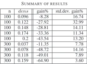
Regarding all the remaining experiments, the results are summarized in Table I.
TABLE I. SUMMARY OF RESULTS
n dens gain% std.dev. gain% 100 0.096 -8.28 16.74 100 0.122 -27.92 32.99 100 0.148 -28.81 14.11 100 0.174 -33.36 11.34 100 0.2 -43.54 13.20 300 0.037 -11.35 7.78 300 0.078 -48.72 14.16 300 0.118 -49.01 7.89 300 0.159 -64.90 3.60
Each row represents a set of experiments characterized by a test configuration. The first two values represent the number of nodes and the density of the networks. For each test configuration, at least 20 experiments have been performed by taking different values of k in the range
0.02m to0.16m. The remaining two columns report the average values gain% and their standard deviations. No-tice that the values of gain% are negative, meaning that, in average, BF.1 performs better than DECR. However, the extra number of messages used by DECR can be seen as the price to avoid space consumption, looping and count-to-infinity phenomena.
v s
b a
1
1 1
1
v s
b a
100
1 1
1
Figure 9. A graphGbefore and after a weight increase on edge(s, v).
botha andb, but only the estimated distances. For each updating step the estimated distances increase by 1 (i.e., the weight of the edge (a, b)). The counting stops after a number of updating that depends on the new weight of the edge(u, v). If the new weight is∞- that is, the link
(u, v)breaks - then the algorithm counts to infinity. Conversely, DECR requires few steps to update both the estimated distance and via tosfor each node inG. When
sandvdetect the weight change, they perform Procedure INCREASEwith respect sources. In particular,sdoes not performsBUILD-TABLEphase, whilevdoes. Whenvgets the estimated distances tosfrom its neighbors (Line 6 of Procedure INCREASE), it receives+∞ from both aand
b. This is due to the fact that, whena(b, resp.) performs Procedures DIST, the test at Line 1 returns true. At the end of these executions, v correctly updates its routing table and sends messages increase to each neighbor. Hence,s,
a, and bperform Procedure INCREASE, but onlyaandb
perform the BUILD-TABLE phase. In this phase, aand b
send ∞ (as their estimated distance to s) to each other in response to the get-dist message (see Line 6). This is due to the fact that, during the executions of Procedure DIST, both a and b are performing the BUILD-TABLE
phase and then, the test at Line 1 returns true. Hence, botha andb correctly update their routing tables in one step. Subsequent messages sent byaandbdo not produce further local data modification.
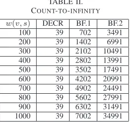
The tests on the example shown in Figure 9 are reported in Table II.
TABLE II. COUNT-TO-INFINITY
w(v, s) DECR BF.1 BF.2 100 39 702 3491 200 39 1402 6991 300 39 2102 10491 400 39 2802 13991 500 39 3502 17491 600 39 4202 20991 700 39 4902 24491 800 39 5602 27991 900 39 6302 31491 1000 39 7002 34991
The results show that DECR requires a constant number of messages, while, as expected, BF.1 and BF.2 require a number of messages that depends on the new weight on the edge (s, v). Notice that, the table shows the total number of messages required by the algorithms, while in the previous discussion we have only considered the
messages required to update the routing table with respect tos.
To conclude our discussion on the performances of the three implemented algorithms, we show the results about the space occupancy. BF.1 requires to store, for each destination, the estimated distance given by each of its neighbors, BF.2 only its estimated distance, whereas DECR is something in between: the estimated distance and the set via. Since it is not common to have more than one via to a destination, the size to store the routing table for DECR is very close to the size required by BF.2.
TABLE III.
SPACE REQUIREMENTS IN THE DECREMENTAL CASE
n dens DECR BF.1 (max) BF.1 (avg) BF.2
100 0.096 206 1900 476 200
100 0.122 203 2300 604 200
100 0.148 201 2500 726 200
100 0.174 201 3100 862 200
100 0.200 201 3300 992 200
300 0.037 607 7500 1677 600
300 0.078 627 12300 3498 600
300 0.118 608 18000 5352 600
300 0.159 604 21300 8634 600
300 0.200 610 25800 8979 600
500 0.023 1006 13500 3005 1000 500 0.067 1010 29000 8470 1000 500 0.111 1009 41500 13935 1000 500 0.155 1010 56000 19565 1000 500 0.200 1009 68000 24950 1000
Table III summarizes the data relative to the space used by the three algorithms, assuming that the cost to store either a destination or an estimated distance is unitary. The third column gives the space used by DECR. In particular, it reports the space consumption of the node with the maximum size of via. BF.1 requires much more space (that is given by ntimes the degree of each node): the fourth column reports the space consumption of the node with maximum degree while the average space consumption per node is listed in the fifth column. The last columns gives the space used by BF.2 for each node. This value is given by two timesn.
0 50000 100000 150000 200000 250000 300000 350000 400000 450000
0 20 40 60 80 100 120 140 160 180 200 Number of decreases
Message exchange comparison (n=100; dens=0.0964)
INCR BF.3
Figure 10. Number of messages needed by INCR and BF.3
Since, the space required by the two algorithms is the same, then we just focus on the number of messages they send.
In Figure 10 we report the number of messages used by the two algorithms when n= 100 and dens= 0.0964. The average number of messages required by INCR is always less than that required by BF.3. The gain%, defined in this case as
m(BF.3)−m(IN CR)
m(BF.3)
is about 15% and it is shown in Figure 11.
0 5 10 15 20
0 20 40 60 80 100 120 140 160 180 200
Number of decreases
Message exchange percentage gain (n=100; dens=0.0964)
Figure 11. Message exchange percentage gain in the incremental case
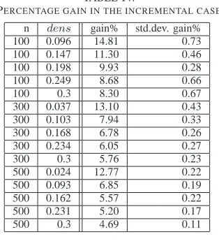
We repeated the experiments for many different test con-figurations, always reaching results qualitatively similar to those shown in Figure 10. These results are summarized in Table IV. Each row in the table refers to at least 40 tests and it is worth to note that the gain% is always in favor of INCR.
TABLE IV.
PERCENTAGE GAIN IN THE INCREMENTAL CASE
n dens gain% std.dev. gain% 100 0.096 14.81 0.73 100 0.147 11.30 0.46
100 0.198 9.93 0.28
100 0.249 8.68 0.66
100 0.3 8.30 0.67
300 0.037 13.10 0.43
300 0.103 7.94 0.33
300 0.168 6.78 0.26
300 0.234 6.05 0.27
300 0.3 5.76 0.23
500 0.024 12.77 0.22
500 0.093 6.85 0.19
500 0.162 5.57 0.22
500 0.231 5.20 0.17
500 0.3 4.69 0.11
VI. FUTURE WORK
Future work will explore the possibility to extend the partially dynamic solutions proposed here to the more realistic fully dynamic case, while keeping the merits of the partially dynamic solution that is: being concurrent
and, in many cases, free of the looping and count-to-infinity phenomena. Another research direction is that of experimentally compare our solution with other variants of the Bellman-Ford methods known in the literature.
REFERENCES
[1] G. D’Angelo, S. Cicerone, G. D. Stefano, and D. Fri-gioni, “Partially dynamic concurrent update of distributed shortest paths,” in International Conference on Computing:
Theory and Applications (ICCTA’07). IEEE Computer
Society, 2007, pp. 32–38.
[2] J. T. Moy, OSPF - Anatomy of an Internet routing protocol. Addison-Wesley, 1998.
[3] H. Attiya and J. Welch, Distributed Computing. John Wiley and Sons, 2004.
[4] D. Frigioni, A. Marchetti-Spaccamela, and U. Nanni, “Fully dynamic algorithms for maintaining shortest paths trees.” Journal of Algorithms, vol. 34, no. 2, pp. 251–281, 2000.
[5] G. Ramalingam and T. Reps, “On the computational com-plexity of dynamic graph problem.” Theoretical Computer
Science, vol. 158, pp. 233–277, 1996.
[6] C. Demetrescu and G. F. Italiano, “A new approch to dynamic all pairs shortest paths.” Jou. of ACM, vol. 51, no. 6, pp. 968–992, 2004.
[7] B. Awerbuch, I. Cidon, and S. Kutten, “Communications-optimal maintenance of replicated information.” in Proc.
IEEE Symposium on Foundation of Computer Science,
1990, pp. 492–502.
[8] S. Cicerone, G. D. Stefano, D. Frigioni, and U. Nanni, “A fully dynamic algorithm for distributed shortest paths.”
Theoretical Computer Science, vol. 297, no. 1-3, pp. 83–
102, Mar. 2003.
[9] P. A. Humblet, “Another adaptive distributed shortest path algorithm.” IEEE Transactions on Communications, vol. 39, no. 6, pp. 995–1002, Apr. 1991.
[10] G. F. Italiano, “Distributed algorithms for updating short-est paths.” Proceedings of Int. Workshop on Distributed
Algorithms., vol. LNCS, 579, pp. 200–211, 1991.
[11] A. Orda and R. Rom, “Distributed shortest-path and minimum-delay protocols in networks with time-dependent edge-length.” Distributed Computing, vol. 10, pp. 49–62, 1996.
[12] K. V. S. Ramarao and S. Venkatesan, “On finding and up-dating shortest paths distributively.” Journal of Algorithms, vol. 13, pp. 235–257, 1992.
[13] J. McQuillan, “Adaptive routing algorithms for distributed coomputer networks,” Cambridge, MA, Tech. Rep. BBN Report 2831, 1974.
[14] D. Bertsekas and R. Gallager, Data Networks. Prentice Hall International, 1992.
[15] A. S. Tanenbaum, Computer Networks. Prentice Hall, 1996.
[16] E. C. Rosen, “The updating protocol of arpanet’s new routing algorithm.” Computer Networks, vol. 4, pp. 11–19, 1980.
[17] B. Awerbuch, A. Bar-Noy, and M. Gopal, “Approximate distributed bellman-ford algorithms.” IEEE Transactions
on Communications, vol. 42, no. 8, pp. 2515–2517, 1994.
[18] S. Cicerone, G. D’Angelo, G. Di Stefano, and D. Frigioni, “Partially dynamic efficient algorithms for distributed shortest paths,” ARRIVAL Project, Tech. Rep. 0022, 2006. [19] “OMNeT++: the discrete event simulation environment.”
http://www.omnetpp.org/.
Serafino Cicerone received his Ph.D. in February 1998 from the University of Rome ”La Sapienza”. He has been visiting scientist at the Institute of Theoretical Computer Science, University of Rostock (Germany). Currently he is associate professor in Computer Science at the University of L’Aquila. His main research areas concern network algorithms, combinatorial optimization, algorithmic graph theory, and he is (co-)author of several papers published in both international journals and conferences. He has con-tributed to the organization of international and national conferences. He participated and participates in several EU and national funded projects.
Gianlorenzo D’Angelo is currently a Ph.D. student in the Department of Electrical and Information Engineering of the University of L’Aquila. His research interests are in the area of graphs and networks algorithms. In particular, he is involved in the development of sequential and distributed algorithms for the shortest paths problem in a dynamic environment.
Gabriele Di Stefano obtained his Ph.D. at the University ”La Sapienza” of Rome in 1992. Currently he is asso-ciate professor for computer science at the University of L’Aquila; his current research interests include network algorithms, combinatorial optimization, algorithmic graph theory; he is (co-)author of more than 50 publications in journals and international conferences. He had key-participation in several EU funded projects. Among them: MILORD (AIM 2024), COLUMBUS (IST 2001-38314), AMORE (HPRN-CT-1999-00104), and, currently, AR-RIVAL (IST FP6-021235-2).
Daniele Frigioni received his Ph.D. in February 1997 by the University of Rome ”La Sapienza”. He his currently associate professor for computer science at the University of L’Aquila (Italy). His main research areas concern the design, analysis and engineering of graph and network algorithms. He is (co-)author of several publications in this area in both international journals and conferences. He has contributed to the organization of several inter-national and inter-national conferences. He participated and participates in several EU and national funded projects. (http://www.diel.univaq.it/frigioni)