Ensemble Dynamics in Non-stationary Data Stream Classification

(1)

Stream Classification

Hossein Ghomeshi, Mohamed Medhat Gaber and Yevgeniya Kovalchuk

AbstractData stream classification is the process of learning supervised models from continuous labelled examples in the form of an infinite stream that, in most cases, can be read only once by the data mining algorithm. One of the most chal-lenging problems in this process is how to learn such models in non-stationary en-vironments, where the data/class distribution evolves over time. This phenomenon is called concept drift. Ensemble learning techniques have been proven effective adapting to concept drifts. Ensemble learning is the process of learning a number of classifiers, and combining them to predict incoming data using a combination rule. These techniques should incrementally process and learn from existing data in a limited memory and time to predict incoming instances and also to cope with different types of concept drifts including incremental, gradual, abrupt or recurring. A sheer number of applications can benefit from data stream classification from non-stationary data, including weather forecasting, stock market analysis, spam fil-tering systems, credit card fraud detection, traffic monitoring, sensor data analysis in Internet of Things (IoT) networks, to mention a few. Since each application has its own characteristics and conditions, it is difficult to introduce a single approach that would be suitable for all problem domains. This chapter studies ensembles’ dy-namic behaviour of existing ensemble methods (e.g. addition, removal and update of classifiers) in non-stationary data stream classification. It proposes a new, compact, yet informative formalisation of state-of-the-art methods. The chapter also presents results of our experiments comparing a diverse selection of best performing

algo-Hossein Ghomeshi

School of Computing and Digital Technology, Birmingham City University e-mail: [email protected]

Mohamed Medhat Gaber

Yevgeniya Kovalchuk

(2)

rithms when applied to several benchmark data sets with different types of concept drifts from different problem domains.

1 Introduction

Over the past few years, data stream classification has been playing an important role in the area of knowledge discovery and big data analytics. The goal of classification, in the context of data streams, is to predict the class label of incoming instances from continuous data records that, generally, can be read only once in a limited time and memory. This is done by extracting useful knowledge from the past data inside the stream by using machine learning techniques.

As our digital world is growing rapidly, there are more data available in the form of data streams (e.g. World Wide Web, Internet of Things, etc.). That fact justifies the importance of paying attention to the mentioned domain of research since knowledge discovery is more complex in data streams. Suppose a sensor net-work that produces data related to credit card transactions of a bank from different types of devices (ATM, POS, online shopping, etc.) in the form of a data stream. A credit card fraud detection system can detect the fraudulent transactions using a data stream classification technique. The same task usually takes a long time or a high cost of resources (manual works) in traditional systems. Other applications of data stream classification include stock market analysis and prediction, weather forecasting, spam detection and filtering, traffic and forest monitoring, electricity management systems, web search pattern detection, sensor data analysis in an Inter-net of Things (IoT) Inter-network, among many other applications.

In such tasks, the characteristics of different types of data streams should be taken into careful consideration in order to have a successful data stream classification. General characteristics of data streams as seen by [Babcock et al., 2002] includes the unlimited size of data streams, on-line arrival of data elements, order of data elements that is not governable, and finally, the restrictions about processing the elements only one time (it is possible to process an element more than once, but with a high cost of storing elements).

From the data distribution point of view, there are two types of data streams: stationary(stable) data streams, where the probability distribution of instances is fixed, and non-stationary(evolving) data streams, where the probability distribu-tion of incoming data evolves or target concepts (labelling mechanism) change over time. This later phenomena is called concept drift. Existence of concept drifts in data streams makes classification tasks more complex and difficult to handle. This chapter is focused on non-stationary data stream classification.

(3)

occur when the data distribution changes and stays in a new distribution after going through some new, unstable, median data distributions. In gradual concept drifts, the amount of new probability distribution of incoming data increases, while the amount of data that belong to the former probability distribution decreases over time. Recur-ring concepts happen when the same old probability distribution of data reappears after some time of a different distribution.

Fig. 1 Different types of concept drifts. Adapted from [Gama et al., 2014].

In order to cope with the concept drift problem in a data stream, it is important to build a classification system that adapts to different concept drifts as quickly as possible.Ensemble learningtechniques are among the most effective approaches to do data stream classification [Gomes et al., 2017], especially when dealing with non-stationary environments and concept drifts [Krawczyk et al., 2017].

Ensemble learning is a machine learning approach in which multiple classifiers are created and combined with each other using a voting mechanism. In other words, as can be seen in Figure 2, a voting mechanism is used to combine different classi-fiers’ outputs in order to establish a single class label as the output of the ensemble. This is done in order to cover different types of features in a data stream. The com-bination is usually done by majority voting or weighted majority voting.

Adaptation to concept drifts can be achieved via different methods, with the most common ways being adding new classifiers into the ensemble, removing old classi-fiers from it, updating the weights of classiclassi-fiers (assigning higher weights for more accurate classifiers at each iteration) and resetting the ensemble to an initial state. All of these methods are related to the dynamic behaviour of the ensemble.

(4)

for-Fig. 2 An ensemble learning system, adapted from [Krawczyk et al., 2017].

malisation of the state-of-the-art methods. The authors argue that understanding the dynamic behaviour of different ensembles, along with the introduced formalisation, can facilitate the development of new as well as the current ensembles.

The rest of this chapter is organized as follows. In Section 2, the current ensem-ble approaches for non-stationary environments are introduced and their dynamic behaviour is discussed. A novel taxonomy for classification in such environments based on dynamic behaviour is proposed in Section 2. A formalisation, along with some of the current ensemble techniques (based on their dynamism diversity) using the proposed formalisation, are included in Section 3. In Section 4, the experimen-tal results of several ensemble techniques are presented and analysed using different data sets. In Section 5, the observed behaviour of different mechanisms is discussed and several suggestions are proposed with respect to various characteristics. Finally, a summary of the experiments, along with some recommendations regarding the application of each ensemble approach, are provided in Section 6.

2 Ensemble Dynamics

In non-stationary environments, where different types of concept drifts may hap-pen, it is expected that an ensemble adapts to a new concept drift swiftly. Since the adaptation in such environments is being done by adding a new classifier to the ensemble, removing old classifiers and changing the weights of current classifiers, understanding the dynamic behaviour of an ensemble toward different types of con-cept drifts can help us to choose the best approach for a specific application domain and develop new ensemble learning techniques for the required purpose.

(5)

studied and compared for this purpose. It has been tried to include the most recent and diverse ensemble techniques in this study.

2.1 Addition

Adding new classifiers that have been trained with recent instances in a stream is one of the most important actions that needs to be applied to the ensemble when data is evolving. The aim of this operation is adapting to drifting data, as well as improving classification accuracy of the ensemble based on the fact that, in most cases, incoming data is more likely to be similar to upcoming instances. The lack of this action might result in severe decrease in accuracy of the ensemble especially when concept drift is happening. One decision that needs to be taken when making a strategy for the ensemble is to decide when to add new classifiers to the ensemble, or in other words, what time frame needs to be taken for the addition operation. Some algorithms use afixedtime, while others use adynamictime for it.

2.1.1 Fixed time of addition

Algorithms that use a fixed time to train and add new classifiers usually use a similar strategy; they do the addition operation after receiving a new block of data or after receiving a predefinedpinstances. A considerate number of existing algorithms are using this strategy to add new classifiers. The main challenge to build or use such algorithms is to pick a decent size ofblocksorpin order to have the best possible output. Picking a large size might decelerate the adaptation while using a small size might make the ensemble sensitive to noise.

2.1.2 Dynamic time of addition

(6)

All of the studied algorithms and their addition mechanisms are shown in Table 1.

2.2 Removal

Removing classifiers is a strategy to forget previously gained knowledge from a data stream that is unhelpful in the current situation, in order to adjust the ensemble to an updated state. In the majority of cases, removing classifiers from an ensemble happens when a predefined ensemble size is reached. However, in some algorithms, classifiers are being removed when their accuracy drops below a predefined thresh-old. In yet other algorithms, the size of ensemble is set unlimited, hence no classifier will be eliminated from the ensemble unless a pruning method is utilised. In this chapter, the removing strategy of algorithms is categorised into the following four types as can be seen in Table 1:

• Full: is performed when the set ensemble size is reached, and there is a new classifier that needs to be added to the ensemble. Such algorithms eliminate clas-sifiers based of the clasclas-sifiers’ age in the ensemble or their performance on the recent data. All of the algorithms that use this mechanism for removing classifiers are the ones that use ‘fixed’ strategy for adding new classifiers.

• Performance based: is performed when the performance of a classifier in the last predefined k example drops below a specified threshold in the stream. In this mechanism, when a classifier becomes ‘unhelpful’ in a new concept, it is considered as an obsolete classifier and is removed from the ensemble.

• Drift detection based: when a concept drift detection method identifies a ‘concept drift’, a classifier is chosen to be eliminated. According to this approach, when the ensemble is full, for every new concept drift that would be detected by a drift detection method, only one classifier will be eliminated based on its accuracy over the recent instances. This happens in order to make room for a new classifier that needs to be added to the ensemble. All of such algorithms use a detection dynamic mechanism for adding new classifiers.

(7)

2.3 Update

Updating an ensemble can be referred to two main operations: the first one is updat-ing the weight or rankupdat-ing each classifier in the ensemble, and the second is whether or not to train old classifiers with incoming data. Most of the current algorithms use the ‘updating weight’ mechanisms in order to improve accuracy, however, only a few algorithms use the ‘training old classifiers’ mechanism, as a high load of memory is needed to train all of the classifiers with incoming data. The existing algorithms and their updating strategies are depicted in Table 1.

Updating the power of each classifier is an efficient way of improving the accu-racy of an ensemble, especially when a concept drift happens and there are diverse classifiers in the ensemble. This is usually done by evaluating the positive effective-ness of each classifier in an environment and changing the weight, or the rank, of the classifier, so that the classifier with a higher accuracy towards the current condition has a bigger impact to the ensembles output than a weaker classifier. Note that the algorithms that use a simple majority voting method for selecting the output of the ensemble are unable to employ this procedure, as there is no weight or rank set for each classifier. Similar to the addition stage, the mechanisms for updating weights of classifiers are categorised tofixedtimes anddynamictimes. The methods that use dynamic times for updating classifiers are usually used when a drift is detected, ex-cept for AddExp algorithm [Kolter & Maloof, 2005], where updating is done when a classifier misclassified an example.

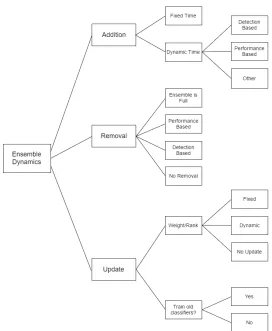
2.4 Ensemble Dynamics Taxonomy

To summarise the above operations, we propose a taxonomy for defining ensemble’s dynamics in non-stationary data stream classification (Figure 3). According to the proposed taxonomy, the dynamic behaviour of ensemble techniques is categorised into three main sections of addition, removal and update as mentioned in Section 2. The addition mechanisms are partitioned into fixed and dynamic methods and dynamic ones are then divided into detection based, performance based and others (such as using acceptance factor, etc.). The removal techniques are partitioned into full (which remove a classifier whenever the ensemble is full), performance based, detection based and no removal (methods that do not remove classifiers). Finally, the update section is divided into two subsections of updating the classifiers’ weights (or ranks) and training old classifiers. The first updating subsection is partitioned into fixed times, dynamic times and no update, while the second one (training) is simply divided into the algorithms that do train the old classifiers (yes) and the ones that do not do so (no).

(8)

, Dynamic Weighted Majority (DWM) [Kolter & Maloof, 2007], Track Recurring Ensemble (TRE) [Ramamurthy & Bhatnagar, 2007], Adwin Bagging (AdwinBag) [Bifet et al., 2009], Recurring Concept Drift (RCD) [Gonc¸alves Jr & De Barros, 2013] and Online Accuracy Update Ensemble (OAUE) [Brzezinski & Stefanowski, 2014a]. These algorithms and their dynamic characteristics are shown in Figure 4. As can be observed from Figure 4, none of the chosen algorithms follow the same path across all four phases of addition, removal, updating and training. Furthermore, there are no two algorithms with more than two common dynamic characteristics in this selection.

(9)

Table 1 Overview of dynamic behaviour of studied algorithms

Algorithm Addition Removal Update Train Reference

SEA Fixed Full No update No [Street & Kim, 2001] AWE Fixed Performance Fixed No [Wang et al., 2003] CDC Other Performance Fixed No [Stanley, 2003] Aboost Fixed Full Dynamic No [Chu & Zaniolo, 2004] CBEA Fixed Full No update No [Rushing et al., 2004] AddExp Misclassify No removal Dynamic No [Kolter & Maloof, 2005] ACE Detection No removal Dynamic No [Nishida & Yamauchi, 2007] DWM Misclassify Performance Fixed Yes [Kolter & Maloof, 2007] TRE Other No removal Fixed No [Ramamurthy & Bhatnagar,

2007]

Adwin Bag Detection Detection No update No [Bifet et al., 2009] BWE Detection Detection Fixed No [Deckert, 2011] Learn++ Fixed No removal Fixed No [Elwell & Polikar, 2011] Heft-Stream Fixed Full Fixed No [Nguyen et al., 2012]

WAE Fixed Full Fixed No [Wo´zniak, 2013]

RCD Detection No removal Dynamic No [Gonc¸alves Jr & De Barros, 2013]

DACC Fixed Full Fixed Yes [Jaber, 2013]

ADACC Fixed Full Fixed Yes [Jaber, 2013]

AUE Fixed Full Fixed Yes [Brzezinski & Stefanowski, 2014b]

OAUE Fixed Full Fixed Yes [Brzezinski & Stefanowski, 2014a]

Fast-AE Fixed Full Fixed No [Ort´ız D´ıaz et al., 2015]

Legends. Fixed: Fixed time of adding/updating the classifiers, Detection: Detection based (dynamic) times, Misclassify: Misclassified based (dynamic) times of adding classifiers, Full: Removing old classifier when the ensemble size is full, Performance: removing when the performance of a classifier drops from the predefined threshold.

3 Formalisation

Formalising algorithms is a suitable way to comprehend and modulate the existing approaches in order to develop novel methods. In this chapter, a formalised version of the selected algorithms (as specified in Section 2) is presented with the intention to simplify the process of examining and building new approaches.

The following functions are used in the presented algorithms. Note that the se-quence of the functions is the matter of importance in this formalisation, and the specific implementation of each function might be different for every algorithm.

• Classify(): The ensemble classifies data according to its combinational rule (e.g., weighted majority vote or majority vote).

• Eval(): Evaluating the whole ensemble or classifiers using an evaluation method.

• Update(): Updating the weights (or ranks) of all or one classifier with regards to its own evaluation and updating mechanism.

(10)

Fig. 4 Selected algorithms diversity in addition, removal and updating phases.

• Add(): Adding the newly built classifier to the ensemble.

• Remove(): Removing one or some classifiers based on the ensemble’s specific removal mechanism.

• Train(): Training all or some old classifiers using the new data or data block.

• DriftDetection(): Detecting drifts using a concept drift detection method.

Adaptive boosting (Aboost) algorithm [Chu & Zaniolo, 2004] presented in Algo-rithm 1 takes blocks of data, classifies the instances and then evaluates the ensem-ble’s performance. If a concept drift is detected, it updates all the classifiers and assigns the default weight of ‘one’ to them. Otherwise, it assigns a weight to each instance in the block according to whether or not that instance has been classified correctly (lines 8-9). If an instance is misclassified, a higher weight would be as-signed. If the instance is classified correctly, the default weight of ‘one’ would be assigned. Finally, the oldest classifier in the ensemble will be removed and a new classifier will be built and added to the ensemble (based on the weighted instances in the block).

(11)

Algorithm 1:ABOOSTAdaptive Boosting Algorithm Input:Continuous data blocks,DB={db1,db2,..,dbn}

Output:C: A set of classifiersc={c1,c2,..,cm}and their corresponding weights

w={w1,w2,..,wm}

1 i:=1

2 whiledata stream is not emptydo 3 Classify(dbi)

4 Eval(Ensemble)

5 ifDriftDetection()=1 (drift is detected)then

6 Update(c)

7 else

8 Eval(dbi) 9 Update(dbi) 10 Build(ci+1)

11 Add(ci+1)

12 Remove() //remove oldest classifier

13 i=i+1

this period, all the weights will be normalised and the classifiers with lower weights than a threshold (θ) will be removed from the ensemble. Finally, when the ensemble misclassifies an instance, a new classifier will be built and added to the ensemble. Note that all classifiers are trained incrementally with incoming samples.

In Tracking Recurrent Ensemble algorithm (TRE) [Ramamurthy & Bhatnagar, 2007], a new classifier will be added only when the ensemble error reaches a pre-defined permitted error (τ). Each classifier’s weight would be updated once its per-formance drops below an acceptance factor (θ). This approach does not remove old classifiers unless a pruning method is used. The formalised version of this algorithm is depicted in Algorithm 3

Adwin Bagging (AdwinBag) [Bifet et al., 2009] is an approach that uses a con-cept drift detection method to specify when a new classifier is needed. When the new classifier is built and there is no more room in the ensemble, the worst performing classifier will be removed in order to make room for the new one. The formalised version of this algorithm is shown in Algorithm 4.

(12)

Algorithm 2:DWM Dynamic Weighted Majority algorithm Input:A Data Stream,DS={d1,d2,..,dn}

li: Real label of theith_example 1 Θ: Threshold for removing classifiers

2 p: specified period for addition, removal and update of classifiers.

Output:A set of classifiersc={c1,c2,..,cm}and their corresponding weights

w={w1,w2,..,wm} 3

4 i:=1

5 whiledata stream is not emptydo

6 forj=1toj=mdo

7 Classify(di)

8 ifOutput(bj)6=liand i mod p=0then

9 Update()

10 ifi mod p=0then 11 whilewj<θdo

12 Remove(cj)

13 Train(cj)

14 ifClassify(di)6=lithen 15 Build()

16 Add()

17 i:=i+1

Algorithm 3:TRE Tracking Recurrent Ensemble Input:Continuous data blocks,DB={db1,db2,..,dbn} τ: Permitted errorθ: Acceptance factor

w={w1,w2,..,wm}

1 i:=1

4 forj=1toj=mdo

5 Eval(cj)

6 ifEval(cj)<θthen 7 Update(cj) 8 Eval(Ensemble)

9 ifEnsemble error>τthen

10 Build()

11 Add()

(13)

Algorithm 4:ADWINBAGAdwin Bagging algorithm Input:A Data Stream,DS={d1,d2,..,dn}

M: Ensemble size

Output:A set of classifiersc={c1,c2,..,cm}

1 i:=1

2 whiledata stream is not emptydo 3 Classify(di)

4 ifDriftDetection()=1then

5 Build()

6 Add()

7 forj=1toj=mdo

8 Eval(cj)

9 ifEnsemble size = Mthen

10 Remove() //remove worst performing classifier

11 i:=i+1

using the last classifier. In this approach, only one classifier is active at a time and does the classification task.

Algorithm 5:RCD Recurring Concept Drift framework Input:A Data Stream,DS={d1,d2,..,dn}

Output:A set of classifiersc={c1,c2,..,cm}, Buffer listb={b1,b2,..,bm} 1 ca= Active classifier,ba= Active buffer

2 cn= New classifier,bn= New buffer

3 i:=1

4 whiledata stream is not emptydo 5 Classify(di)

6 DriftDetection() 7 switchDrift Detectiondo

8 caseDriftDetection()= Warning and cn=nulldo 9 Build(cn)

10 Build(bn)

11 caseDriftDetection()= Warning and cn6=nulldo 12 Train(cn)

13 caseDriftDetection()= Driftdo

14 ca←cn

15 ba←bn

16 otherwise do

17 cn=bn=null

18 i:=i+1

(14)

based on their error in constant time and memory. Since this approach needs a high load of memory due to training all classifiers with incoming data, a threshold for memory is assigned – so that, whenever the threshold is met, a pruning method is used to decrease the size of classifiers. The formalised version of this approach is depicted in Algorithm 6.

Algorithm 6:OAUE Online Accuracy Updated Ensemble algorithm Input:A continuous blocks of data,DB={db1,db2,..,dbn}

M: Ensemble size,θ: Memory threshold

w={w1,w2,..,wm}

1 i:=1

4 Eval(c) 5 Build(ci)

6 ifi<Mthen

7 Add(ci)

8 else

9 Remove() //remove least accurate classifier

10 Add(ci)

11 forj=1toj=mdo

12 Update(cj) 13 Train(cj)

14 ifMemory usage>θthen

15 Prune(c) //decrease size of classifiers

16 i:=i+1

4 Experimental Study

To evaluate and analyse the selected algorithms (as specified in Section 2), and to observe the behaviour of different mechanisms with respect to various concept drifts, a set of experiments are conducted using several data sets. For this purpose, two artificial and two real world data streams are employed and the algorithms are compared using different criteria including classification accuracy, training time, memory usage, average adaptation time to concept drifts and average accuracy drop upon concept drifts. Each evaluation run in these experiments involves passing one of the chosen data sets described below through a specific algorithm in a form of data stream with a specified number of instances per interval.

(15)

DWM, OAUE and AdwinBag algorithms are already included in MOA framework and TRE and RCD algorithms are added usingclassifiers and drift detection meth-odsextension1. The experiments were performed on a machine equipped with an Intel Core i7-4702MQ CPU @ 2.20GHz and 8.00 GB of Installed memory (RAM).

4.1 Data Sets

Hyperplane Generator

Hyperplane generator is a synthetic data stream with drifting concepts based on a rotating hyperplane. A hyperplane in d-dimensional space is the set of points that satisfy

d

∑

i=1

wixi=w0wherexi is theith coordinator of pointx. Instances with d

∑

i=1

wixi≥w0are labelled as positive and

d

∑

i=1

wixi<w0are labelled as negative.

Ro-tating Hyperplane Generator was introduced by [Hulten et al., 2001] and is a good way to simulate concept drift by changing the location of the hyperplane and addi-tionally to change the smoothness of drifting data by specifying the magnitude of the changes.

For this experiment, the number of classes and attributes are set to four and four-teen respectively, and the magnitude of change is set to 0.01.

SEA Data Stream Generator

SEA generator is a data set inspired by four SEA concepts as described in [Street & Kim, 2001]. The data set is a set of random points in a three-dimensional feature space. All three features have the value between 0 to 10, but only the first two are relevant to classification. These points are then divided into four blocks with differ-ent concepts. This is done to specify differdiffer-ent concept drifts by assigning differdiffer-ent conditions and goals for each class.

For this experiment along with the normal concept drifts that are being generated in the data stream, three abrupt concept drifts are added manually in three predefined times in order to be able to analyse the behaviour of different algorithms in the exact same situation specifically towards abrupt concept drifts.

(16)

Forest Cover-type Data Set

Forest Cover-type data set [Blackard & Dean, 1999] from the UCI Machine Learn-ing Repository2_{contains the forest cover type of 30}_×_{30 meter cells obtained from}

the US Forest Service (USFS) Region 2 Resource Information System (RIS) data. It contains 581,012 instances and 54 attributes. The goal with this data set is to predict the forest cover type from cartographic variables.

Electricity Data Set

Electricity is a widely used data set by [Harries & Wales, 1999] collected from the Australian New South Wales Electricity Market. In this market, prices are not fixed and are affected by demand and supply. The Electricity data set contains 45,312 in-stances. Each instance contains 8 attributes and the target class specifies the change of the price (whether going up or down) according to a moving average of the last 24 hours.

4.2 Results and Analysis

To evaluate performance of the selected algorithms, three generic criteria are used, including ‘Accuracy’, ‘Execution time’ and ‘Memory usage’. Accuracy is the per-centage of correctly classified instances in the given interval. Execution time and memory usage represent how much time and memory overall it takes for an al-gorithm to complete an evaluation run. For the second experiment with SEA data stream, two more criteria are utilised in order to study algorithms’ behaviour in the presence of abrupt concept drift. These criteria are accuracy drop upon a concept drift and recovery time from a concept drift (adaptation time). Accuracy drop is calculated as a ratio (in %) between the last interval’s accuracy rate before the new drift is introduced and the next interval’s accuracy rate. Recovery time is the aver-age number of instances it takes for each algorithm to achieve its averaver-age accuracy again (after an abrupt concept drift).

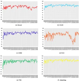
Figure 5 shows the percentage of classification accuracy of the selected algo-rithms over Hyperplane data set. Algoalgo-rithms’ behaviour in identical scenarios are demonstrated in Figure 6. The elapsed time and memory usage are shown in Fig-ures 7 and 8.

Accuracy rates of the selected algorithms over SEA generator data stream are shown in Figure 9. In order to create abrupt concept drifts at specified times, one million instances are generated from SEA data generator [Street & Kim, 2001] with

(17)

Fig. 5 Classification accuracy of different algorithms for Hyperplane data stream generator (1 million instances). X-axis: Instance number; Y-axis: Accuracy in %(calculated every 5000 in-stances). (a): Adaptive Boosting algorithm, (b): Online Accuracy Updated Ensemble, (c): Dynamic Weighted Majority algorithm, (d): Recurring Concept Drift framework, (e): Tracking Recurrent Ensemble, (f): Adwin Bagging algorithm.

three different parameters that happen every 250 thousand instances. Figure 10 com-pares algorithms’ accuracy rates in one chart.

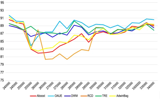
Figure 11 demonstrates behaviour of the tested algorithms towards one of the added abrupt concept drifts. In Figure 12, the selected algorithms are compared ac-cording to their accuracy drop, recovery time, average accuracy, average memory usage and the overall time of an experiment.

(18)

Fig. 6 Comparison of algorithms’ accuracy rates over Hyperplane generator.

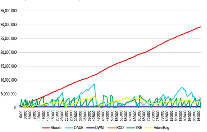
Fig. 7 Overall execution time of the selected algorithms over Hyperplane data generator (in sec-onds).

shown in Figures 15 and 16 respectively. Average accuracy, performance compari-son, memory usage and overall execution time of all algorithms over Electricity data set is demonstrated in Figures 17, 18, 19 and 20 respectively.

(19)

Fig. 8 Memory usage of the selected algorithms (calculated every 5000 instances). X-axis: In-stance number; Y-axis: Memory in bytes.

(20)

us-Fig. 9 Classification accuracy of the algorithms over SEA data stream generator (1 million in-stances). X-axis: Instance number; Y-axis: Accuracy rate (calculated every 5000 instances in %). (a): Adaptive Boosting algorithm, (b): Online Accuracy Updated Ensemble, (c): Dynamic Weighted Majority algorithm, (d): Recurring Concept Drift framework, (e): Tracking Recurrent Ensemble, (f): Adwin Bagging algorithm.

(21)

Fig. 10 Comparison of algorithms’ accuracy rates over SEA generator.

Fig. 11 A closer look at one of the added abrupt concept drifts and the behaviour of different algo-rithms towards this drift. X-axis: Instance number; Y-axis: Classification accuracy rate (calculated every 5000 instances in %).

5 Discussion

(22)

Fig. 12 Comparison of the algorithms in SEA generator data stream in the presence of different concept drifts in 1 million instances. (a): Average accuracy in %, (b): Average drop of accuracy upon concept drifts, (c): Average time of recovery (adaptation) from concept drift (number of instances to pass in order to achieve the average performance again), (d): Overall time, (e): Average memory usage.

(23)

Fig. 13 Classification accuracy of the tested algorithms over the Forest Cover-type data set (581,012 instances). X-axis: Instance number, Y-axis: Accuracy rate (calculated every 2000 in-stances in %). (a): Adaptive Boosting algorithm, (b): Online Accuracy Updated Ensemble, (c): Dynamic Weighted Majority algorithm, (d): Recurring Concept Drift framework, (e): Tracking Recurrent Ensemble, (f): Adwin Bagging algorithm.

for other algorithms, accuracy remains the same or increases. This can be explained by inability of the algorithms to distinguish between the true signal and noise. In the instance number 775000, the accuracy of all algorithms drop smoothly, while in Aboost and especially RCD this drop is more severe. Furthermore, in Figure 5, it is clear that accuracies of OAUE and DWM algorithms (b,c) have the lowest rate of fluctuation among the others. This is possibly the result of training old classifiers as new examples are passing through the ensemble.

(24)

Fig. 14 Comparison of algorithms’ accuracy rates over the Forest Cover-type data set.

Fig. 15 Memory usage of the selected algorithms over Forest Cover-type data set (calculated every 2000 instances). X-axis: Instance number, Y-axis: memory used (in bytes).

(25)

clas-Fig. 16 Overall execution time of the selected algorithms over Forest Cover-type data set (in sec-onds).

Table 2 Overview of all experiments with respect to accuracy, execution time and memory usage.

— Average Accuracy (%) Execution Time (second) Memory Usage (KB) Algorithm Plane SEA Forest Elec Plane SEA Forest Elec Plane SEA Forest Elec Aboost 87.56 87.91 75.48 89.77 188 46 184 4 14807 3515 5631 550 OAUE 90.69 89.42 90.11 87.5 128 49 164 3.98 2888 2754 1947 844 DWM 89.66 87.87 80.26 70.73 247 58 317 5.48 609 249 932 330 RCD 84.7 86.2 62.66 73.45 34 5 62 1.98 4.4 1.1 24.7 2.6 TRE 88.33 88.05 77.3 71.68 1378 260 1509 8.77 1924 694 3423 666 AdwinBag 90.06 88.17 84.81 84.34 86 46 124 2.97 2059 2612 428 238

sifiers with incoming data in these algorithms. Similar to the previous experiment (Hyperplane data set), the algorithms that use concept drift detection methods (Ad-winBag, RCD and Aboost) adapt to concept drifts slowly and their accuracy drops drastically upon concept drifts (Figure 12).

(26)

Fig. 17 Classification accuracy of different algorithms over Electricity data set (45,312 instances). X-axis: Instance number; Y-axis: Accuracy rate (calculated every 500 instances in %). (a): Adap-tive Boosting algorithm, (b): Online Accuracy Updated Ensemble, (c): Dynamic Weighted Ma-jority algorithm, (d): Recurring Concept Drift framework, (e): Tracking Recurrent Ensemble, (f): Adwin Bagging algorithm.

drifts, both conditions happen often, which leads to adding new classifiers more frequently.

(27)

Fig. 18 Comparison of algorithms’ accuracy rates over Electricity data set.

Fig. 19 Memory usage of the selected algorithms over Electricity data set (calculated every 500 instances). X-axis: Instance number; Y-axis: Memory in bytes.

some time in order to achieve an initial consistency. Furthermore, it can be noticed from Figure 14 that RCD and Aboost algorithms have inconsistent performance in highly evolving data sets.

(28)

Fig. 20 Overall execution time of the selected algorithms over Electricity data set (in seconds).

and Aboost) are higher and have more stability than the other algorithms. Further-more, in DWM algorithm with average accuracy of 70.7% the performance is not satisfactory. This is possibly due to the addition operation in DWM algorithm hap-pening when an instance is misclassified by the whole ensemble and the removal operation is based on the performance of each classifier at specific times.

As can be seen from Figures 7, 12(c),16 and 20, TRE algorithm has the longest execution time by far. This is due to the fact that in TRE algorithms there is no mech-anism for removing old classifiers and new incoming instances are being compared with previous ones in order to find recurring concept drifts. Furthermore, DWM and OAUE algorithms mostly have the longest time of execution after TRE, since in these algorithms all the classifiers are trained using new data. As opposed to TRE, RCD algorithm has the shortest execution time because in this algorithm, only one classifier is active at a time and a new classifier is being built at the same time. Finally, AdwinBag algorithm has relatively low execution times in all experiments (Table 2), as this approach does not update the weight or rank classifiers.

(29)

all classifiers are incrementally trained. This leads to both algorithms needing a pruning method to shrink the number of classifiers in TRE, and to shrink the size of each classifier in OAUE.

Overall, for applications where the overall accuracy is an important factor and classification time is not restricted, OAUE and Aboost algorithms demonstrate bet-ter results. For applications where memory and time are limited, AdwinBag and RCD algorithms are recommended. In applications where consistency of accuracy is important, algorithms such as TRE, DWM and OAUE should be used. Finally, for applications where good performance upon concept drift is required, TRE and DWM algorithms are recommended as they demonstrate the most consistent results.

6 Summary

In this chapter, dynamic changes of different ensemble-based approaches for data stream classification in non-stationary environments have been studied. A novel tax-onomy has been proposed based on dynamic behaviour of these approaches, in or-der to establish different types of reactions to concept drifts. To simplify the process of understanding the current approaches’ dynamics and to encourage the develop-ment of novel algorithms, a formalisation method for classification algorithms in streaming analytics has been presented and characteristics of some of the current algorithms have been represented using this method. Finally, six algorithms out of the studied twenty algorithms are selected based on their diverse dynamic behaviour and four experiments have been designed for the purpose of this chapter. These ex-periments have been conducted to analyse the consequences of employing different types of dynamic behaviour towards different applications and concept drifts.

Based on the experimental results, the most significant observations are as fol-lows:

• For the tasks where accuracy is the most important factor and the target data stream is being evolved frequently and severely, it is suggested to use algorithms with frequent updating and training phases, such as Aboost, OAUE and DWM.

• For applications where only a small amount of memory is available (such as IoT and sensor networks) or the time of output needs to be short, it is suggested to use RCD, Adwin Bagging and other algorithms with less updating or adding procedures.

• For the applications where frequent recurring concept drifts happen and memory usage is not crucial, algorithms such as TRE algorithm, where no classifier is deleted, are recommended to use.

• For the tasks where the memory capacity is limited and the job needs to be done in a short time with a satisfactory level of accuracy, AdwinBag and DWM algo-rithms are suggested.

(30)

• For applications where recovery time (time of adaptation) is a critical factor, OAUE and DWM algorithms that train all classifiers incrementally seem to be the best option.

• For applications where consistency of accuracy rate is important, algorithms such as DWM, TRE and OAUE that update their classifiers frequently are the best choices.

• For applications where the accuracy over concept drifts is the most important factor, algorithms that add more classifiers or have more ‘adding’ procedures in evolving environments (e.g., misclassified-based and performance-based mecha-nisms of adding), such as TRE and DWM are proved to be the best options.

References

[Babcock et al., 2002] Babcock, Brian, Shivnath Babu, Mayur Datar, Rajeev Motwani, & Jennifer Widom 2002. Models and issues in data stream systems. In Proceedings of the twenty-first ACM SIGMOD-SIGACT-SIGART symposium on Principles of database systems, pages 1–16. ACM. [Bifet et al., 2010] Bifet, Albert, Geoff Holmes, Richard Kirkby, & Bernhard Pfahringer 2010.

Moa: Massive online analysis. Journal of Machine Learning Research, 11(May):1601–1604. [Bifet et al., 2009] Bifet, Albert, Geoff Holmes, Bernhard Pfahringer, Richard Kirkby, & Ricard

Gavald`a 2009. New ensemble methods for evolving data streams. In Proceedings of the 15th ACM SIGKDD international conference on Knowledge discovery and data mining, pages 139– 148. ACM.

[Blackard & Dean, 1999] Blackard, Jock A, & Denis J Dean 1999. Comparative accuracies of artificial neural networks and discriminant analysis in predicting forest cover types from carto-graphic variables. Computers and electronics in agriculture, 24(3):131–151.

[Brzezinski & Stefanowski, 2014a] Brzezinski, Dariusz, & Jerzy Stefanowski 2014a. Combin-ing block-based and online methods in learnCombin-ing ensembles from concept driftCombin-ing data streams. Information Sciences, 265:50–67.

[Brzezinski & Stefanowski, 2014b] Brzezinski, Dariusz, & Jerzy Stefanowski 2014b. Reacting to different types of concept drift: The accuracy updated ensemble algorithm. IEEE Transactions on Neural Networks and Learning Systems, 25(1):81–94.

[Chu & Zaniolo, 2004] Chu, Fang, & Carlo Zaniolo 2004. Fast and light boosting for adaptive mining of data streams. In Pacific-Asia Conference on Knowledge Discovery and Data Mining, pages 282–292. Springer.

[Deckert, 2011] Deckert, Magdalena 2011. Batch weighted ensemble for mining data streams with concept drift. In International Symposium on Methodologies for Intelligent Systems, pages 290–299. Springer.

[Elwell & Polikar, 2011] Elwell, Ryan, & Robi Polikar 2011. Incremental learning of concept drift in nonstationary environments. IEEE Transactions on Neural Networks, 22(10):1517–1531. [Gama et al., 2014] Gama, Jo˜ao, Indr˙e ˇZliobait˙e, Albert Bifet, Mykola Pechenizkiy, & Abdel-hamid Bouchachia 2014. A survey on concept drift adaptation. ACM Computing Surveys (CSUR), 46(4):44.

[Gomes et al., 2017] Gomes, Heitor Murilo, Jean Paul Barddal, Fabr´ıcio Enembreck, & Albert Bifet 2017. A Survey on Ensemble Learning for Data Stream Classification. ACM Computing Surveys (CSUR), 50(2):23.

[Gonc¸alves Jr & De Barros, 2013] Gonc¸alves Jr, Paulo Mauricio, & Roberto Souto Maior De Bar-ros 2013. RCD: A recurring concept drift framework. Pattern Recognition Letters, 34(9):1018– 1025.

(31)

[Hulten et al., 2001] Hulten, Geoff, Laurie Spencer, & Pedro Domingos 2001. Mining time-changing data streams. In Proceedings of the seventh ACM SIGKDD international conference on Knowledge discovery and data mining, pages 97–106. ACM.

[Jaber, 2013] Jaber, Ghazal 2013. An approach for online learning in the presence of concept change. PhD thesis, Citeseer.

[Kolter & Maloof, 2005] Kolter, Jeremy Z, & Marcus A Maloof 2005. Using additive expert ensembles to cope with concept drift. In Proceedings of the 22nd international conference on Machine learning, pages 449–456. ACM.

[Kolter & Maloof, 2007] Kolter, J Zico, & Marcus A Maloof 2007. Dynamic weighted ma-jority: An ensemble method for drifting concepts. Journal of Machine Learning Research, 8(Dec):2755–2790.

[Krawczyk et al., 2017] Krawczyk, Bartosz, Leandro L Minku, Jo˜ao Gama, Jerzy Stefanowski, & Michał Wo´zniak 2017. Ensemble learning for data stream analysis: a survey. Information Fusion, 37:132–156.

[Nguyen et al., 2012] Nguyen, Hai-Long, Yew-Kwong Woon, Wee-Keong Ng, & Li Wan 2012. Heterogeneous ensemble for feature drifts in data streams. Advances in Knowledge Discovery and Data Mining, pages 1–12.

[Nishida & Yamauchi, 2007] Nishida, KYOSUKE, & Koichiro Yamauchi 2007. Adaptive classifiers-ensemble system for tracking concept drift. In Machine Learning and Cybernetics, 2007 International Conference on, volume 6, pages 3607–3612. IEEE.

[Ort´ız D´ıaz et al., 2015] Ort´ız D´ıaz, Agust´ın, José del Campo- Ávila, Gonzalo Ramos-Jiménez, Isvani Fr´ıas Blanco, Yailé Caballero Mota, Antonio Mustelier Hechavarr´ıa, & Rafael Morales-Bueno 2015. Fast adapting ensemble: A new algorithm for mining data streams with concept drift. The Scientific World Journal, 2015.

[Ramamurthy & Bhatnagar, 2007] Ramamurthy, Sasthakumar, & Raj Bhatnagar 2007. Tracking recurrent concept drift in streaming data using ensemble classifiers. In Machine Learning and Applications, 2007. ICMLA 2007. Sixth International Conference on, pages 404–409. IEEE. [Rushing et al., 2004] Rushing, John, Sara Graves, Evans Criswell, & Amy Lin 2004. A coverage

based ensemble algorithm (CBEA) for streaming data. In Tools with Artificial Intelligence, 2004. ICTAI 2004. 16th IEEE International Conference on, pages 106–112. IEEE.

[Stanley, 2003] Stanley, Kenneth O 2003. Learning concept drift with a committee of decision trees. Informe t´ecnico: UT-AI-TR-03-302, Department of Computer Sciences, University of Texas at Austin, USA.

[Street & Kim, 2001] Street, W Nick, & YongSeog Kim 2001. A streaming ensemble algorithm (SEA) for large-scale classification. In Proceedings of the seventh ACM SIGKDD international conference on Knowledge discovery and data mining, pages 377–382. ACM.

[Wang et al., 2003] Wang, Haixun, Wei Fan, Philip S Yu, & Jiawei Han 2003. Mining concept-drifting data streams using ensemble classifiers. In Proceedings of the ninth ACM SIGKDD international conference on Knowledge discovery and data mining, pages 226–235. AcM. [Wo´zniak, 2013] Wo´zniak, Michał 2013. Application of combined classifiers to data stream