R E S E A R C H Open Access
Zero covariation returns
Dilip B. Madan · Wim Schoutens
Received: 26 November 2017 / Accepted: 7 May 2018 /
© The Author(s). 2018Open AccessThis article is distributed under the terms of the Creative Commons Attribution 4.0 International License (http://creativecommons.org/licenses/by/4.0/), which permits unrestricted use, distribution, and reproduction in any medium, provided you give appropriate credit to the original author(s) and the source, provide a link to the Creative Commons license, and indicate if changes were made.
Abstract Asset returns are modeled by locally bilateral gamma processes with zero covariations. Covariances are then observed to be consequences of randomness in variations. Support vector machine regressions on prices are employed to model the implied randomness. The contributions of support vector machine regressions are evaluated using reductions in the economic cost of exposure to prediction residu-als. Both local and global mean reversion and momentum are represented by drift dependence on price levels. Optimal portfolios maximize conservative portfolio val-ues calculated as distorted expectations of portfolio returns observed on simulated path spaces. They are also shown to outperform classical alternatives.
Keywords Bilateral gamma process·Minmaxvar distortion·Conic portfolio theory·Distorted expectation
JEL Classification G10·G11·G12
1 Introduction
A number of recent papers have proposed the view that price processes in active financial markets are pure jump processes with an infinite aggregate jump arrival rate. By way of examples, we cite Madan (2017a), Madan and Schoutens (2017), Madan and Wang (2017), Madan, Schoutens, and Wang (2017). The jumps synthesize unanticipated shocks occurring at surprise times modeled by Poisson arrival times.
D. B. Madan ()
Robert H. Smith School of Business, University of Maryland, College Park 20742, MD, USA e-mail: [email protected]
W. Schoutens
Given the large number of shocks involved, a limit law like the Gaussian law is employed to describe return distributions. As a consequence, the arrival rate of jumps aggregated across all jumps, must be infinite. This hypothesis is maintained here in the context of studying dependencies in price processes. An approach to studying dependence in the context of jump arrival rate specifications using multivariate arrival rates with full support in higher dimensions is presented in Madan (2017b) building on the developments in Buchmann, Madan, and Lu (2016). Alternative approaches include the use of copulas, Kallsen and Tankov (2006), or multivariate time changes, Luciano and Semeraro (2010), or factor structures, Marf`e (2011). By contrast, the hypothesis entertained here is that of zero covariation. It may be reasonable to pos-tulate that even when two markets respond to the same underlying disturbances, they do so at their own timing. As a consequence, a simultaneous jump in both markets, at essentially the same point of time in continuous time, may be too extreme a hypoth-esis. It is therefore supposed here that price processes have zero covariations with no simultaneous jumps. The paper goes on to develop the consequences of zero covari-ation for dependence modeling and portfolio theory. The zero covaricovari-ation hypothesis is consistent with the view expressed in Epps (1979) and further documented in Bonanno, Lillo and Mantegna (2001), that covariance requires time and declines with the horizon.
For zero covariation processes, the first question addressed is how nonzero covari-ances arise at a particular horizon. It is noted that this is possible only if the integrated instantaneous variations are themselves stochastic. In fact, the covariance at the horizon is the covariance of the instantaneous variations integrated over time. A Markovian formulation then models instantaneous variations as functions of the price processes themselves. For the pairwise case reported on in some detail, the instanta-neous variations are taken to depend on the two prices separately or just their ratio. The result is a pure jump Markov process of the type studied in Bass (1988). For applications to option pricing we cite Elliott and Osakwe (2006)
The modeling exercise has to choose a functional form for the dependence of variations on prices and one could begin with a linear representation. However, we anticipate that there may be no dependence for prices in a certain range with correc-tive actions inducing alterations in variations when price levels are in extraordinary or extreme states. The anticipated relation is then nonlinear and a priori, the functional forms involved are not known. For example, positive drifts may arise when prices rise substantially and negative ones when they fall significantly, to reflect momentum, or the other way around for mean reversion. Further, there may be a local mean rever-sion range coupled with momentum if prices go even further out. As one is in fact modeling the dependence of parameters of jump arrival rate functions on prices, the use of unbounded functions like polynomials is inappropriate and even problematic from the perspective of the existence of processes with the specified jump compen-sators or arrival rate functions. In this regard we note the conditions developed in Bass (1988). For the existence of processes, the use of bounded nonlinear functions is appropriate.
functions extracted from a kernel operator that are generally bounded. With a view towards validating the procedure, the proposed methods are first tested on simulated data where the true nonlinear dependence is known apriori and the rsvm procedures are applied to recover the known dependence.
On real market data, local estimates of instantaneous variations are first con-structed using recent daily time series data. The rsvm procedures are then employed to relate these to the time series data on the corresponding prices or their ratios. The specific rsvm method used employs a regularized form of epsilon insensitive optimization.
The typical support vector machine regression creates a linear combination of hun-dreds of selected nonlinear transforms to build a prediction function. The output of a support vector machine regression is a computer program that may be saved and used for predictions. Given a set of predictors using possibly different prediction archi-tectures there is then a need to evaluate and compare prediction qualities. This could be done on the basis of a variety of fit statistics. In judging statistical significance, fit statistics are often penalized on the basis of the number of estimated coefficients. One may note in this regard the Akaike information criteria (Akaike (1973)) in select-ing the order in a time series analysis. However, in an rsvm application it is not clear how these are to be counted and given the large number of nonlinear transforms involved the penalty may get quite large. Furthermore, fit statistics do not provide an assessment of improvements from an economic viewpoint.
For an economic perspective, we turn to developments in two price economies (Madan and Schoutens (2016)) that evaluate the necessary costs of holding risk expo-sures. Basically, the cost of an exposure is the spread cost of entering and exiting the exposure when trading in both directions at adverse terms. The two price economy provides constructions of lower and upper conservative valuations at which positions may be offloaded or acquired. We take as an economic cost the spread between these upper and lower valuations. For the purpose of valuing predictions, one evaluates the economic cost of the prediction residual seen as a risk exposure. In evaluating dif-ferent predictors, attention is focused on the percentage reductions in exposure costs delivered by various models. The percentage cost reduction is an easily interpretable performance metric.
The bilateral gamma process of K¨uchler and Tappe (2008) written as the difference of two independent gamma processes provides such an example, and it is employed here. It is a generalization of the variance gamma model of Madan and Seneta (1990), and Madan, Carr, and Chang (1998) that results in equating the speed or variance rate parameters for the up and down moves.
The nonlinear projections are first conducted using rsvm in one and two dimen-sions. Results are presented for a variety of equity assets, commodities, interest rates, equity indices, and their volatility indices. Examples are provided for when in a pair of assets one or both may mean revert to the other. There are also examples of local mean reversion coupled with one or both developing momentum with respect to the other once the prices have already deviated sufficiently. One may also have momentum occurring locally.
Models of multivariate dependence across many assets are then constructed by forming support vector machine regressions of all four bilateral gamma parameters of motion on all the prices. Path spaces with the estimated model are then gener-ated by simulation for the investment horizon. Optimal portfolios are constructed for the simulated joint returns. The portfolio constructions follow the methods of conic portfolio theory (Madan (2016)) and maximize a conservative lower portfolio valu-ation. Equivalently, they maximize reward less risk, where the reward is the mean and the risk is the upper valuation for the negated centered variate. This upper val-uation is the cost of eliminating risk by accessing the negated centered variate at adverse market terms. The trade-off between reward and risk is one to one as both are in the same units of dollars. Comparative tests of zero covariation dependent conic portfolios with Markowitz mean variance portfolios are presented. It is observed that zero covariation dependent conic portfolios offer a significantly improved investment performance on a variety of metrics.
The steps to be taken in the paper may then be summarized as follows. First, it is established that zero covariation pure jump return processes develop covariance at a positive time horizon only if the arrival rates of jumps vary stochastically over time. When arrival rates are parametrically characterized, the parameters must then be stochastically varying. To ensure the existence of such processes the parame-ters are taken to vary in a compact set. Consequently, their dependence on observed stochastic processes must be given by bounded nonlinear functions. Support vector machine regressions deliver a robust, bounded, nonlinearity. The result is however complex and is delivered as a computer program as opposed to being expressed as an analytical functional form.
A stylized model is first developed to test the ability of support vector machines to capture the true nonlinearity when it is known. This stylized model is then dropped further in the paper. Support vector machine regressions are then applied to validate their ability to capture zero covariation dependence in data for bond returns. The anticipated mean reversion is observed in this context. The methods are extended next to equity and other asset prices.
purpose based on prior studies. The estimation procedure for the model are described in detail. From such estimates one estimates daily the exponential variations or asset price drifts. Support vector machine regressions are then employed to explain the movements in the drifts.
With a view to evaluating the work being done by the computer programs deliv-ered by support vector machine regressions we formulate a measure of the cost of holding prediction residuals. The percentage reductions in economic cost serve as a measure of support vector machine contributions. We then present the results on asset drift prediction and the economic cost reductions achieved by support vec-tor machine regressions.For portfolio construction one needs to explain more than just the asset drifts. The complete dependence of arrival rates must be synthe-sized. Hence we apply support vector machine regressions on all the four bilateral gamma parameters on all prices in the portfolio to build zero covariation dependence structures. Economic cost reductions achieved on all parameters are presented. The dependence modeling is then complete and permits portfolio construction. Optimal portfolios are formed to maximize conservative portfolio values calculated as dis-torted expectations of portfolio returns. Results are shown for two and multi-asset portfolios with monthly rebalancing and woth comparisons to optimal mean variance portfolios.
The outline of the rest of the paper is as follows. Section2presents results on the implications of zero covariation. Section3takes up the use of support vector machine regressions and validates these procedures on a stylized model and its simulated data. The section also presents an analysis of using support vector machine regressions to model the anticipated dependence present in interest rate data. Section4details the construction of daily variations related to estimating the parameters of motion for asset prices. Section5introduces the economic cost of exposure to prediction resid-uals as an economic measure of model performance. Section 6presents bivariate examples of dependence with zero covariation. Section7takes up portfolio theory in a two-asset context. The multi asset portfolio construction is presented in Section8
and includes a comparison with Markowitz investment of regularly rebalanced port-folios. Also presented are monthly rebalanced portfolios over a nine year period for sets of ten randomly selected stocks. Section9concludes.
2 Covariation and covariance
Consider two price processesS1 =(S1(t), t ≥ 0)andS2 =(S2(t), t ≥ 0)that are
pure jump processes and exponentials ofX1=(X1(t), t ≥0)andX2=(X2(t), t ≥0).
The joint arrival rate function for the pair(X1, X2)in the absence of covariation takes
the special form
kX1,X2(ω, t, x1, x2)=k1(ω, t, x1)1x2=0+k2(ω, t, x2)1x1=0,
where the dependence onωis adapted.
(S1(t+h)−S1(t)) =
t <u≤t+h
S1(u )
eX1(u)−1
(S2(t+h)−S2(t)) =
t <u≤t+h
S2(u )
eX2(u)−1,
when the sums on the right side are well defined as is the case for finite variation log price processes. The joint characteristic function at horizonhis given by
φX1(h),X2(h)(u, v)=E
exp(iuX1(h)+ivX2(h))
=E exp h 0 ds ∞ −∞ ∞ −∞
× eiux1+ivx2−1
kX1,X2(ω, s, x1, x2)dx1dx2 .
From the absence of covariation it follows that
∞
−∞ ∞
−∞
eiux1+ivx2−1
kX1,X2(ω, t, x1, x2)dx1dx2
= ∞
−∞
eiux1−1k
1(ω, t, x1) dx1+
∞
−∞
eivx2−1k
2(ω, t, x2) dx2.
The covariance of returns for horizonhis then given by
− ∂2
∂u∂vφX1(h),X2(h)(u, v)|u=v=0+
∂
∂uφX1(h),X2(h)(u, v)|u=v=0
×
∂
∂vφX1(h),X2(h)(u, v)|u=v=0
Evaluating the required derivatives yields the results
∂
∂uφX1(h),X2(h)(u, v)|u=v=0=iE
h
0
ds
∞
−∞x1k1(ω, s, x1) dx1
=iE
h
0
dsv1(ω, s)
∂
∂vφX1(h),X2(h)(u, v)|u=v=0=iE
h
0
ds
∞
−∞x2k2(ω, s, x2) dx2
=iE
h
0
dsv2(ω, s)
, where
v1(ω, s)=
∞
−∞x1k1(ω, s, x1) dx1
v2(ω, s)=
∞
−∞x2k2(ω, s, x2) dx2,
Furthermore,
− ∂2
∂u∂vφX1(h),X2(h)(u, v)|u=v=0=E
h
0
ds
∞
−∞x1k1(ω, s, x1) dx1
h
0
ds
∞
−∞x2k2(ω, s, x2) dx2
=E
h
0
dsv1(ω, s)
h
0
dsv2(ω, s)
.
The covariance is thus given by
Cov(X1(h), X2(h))=E
h
0
dsv1(ω, s)
h
0
dsv2(ω, s)
−E
h
0
dsv1(ω, s)
E
h
0
dsv2(ω, s)
.
Define the integrated instantaneous variations by
Vi(ω, t)=
t
0
dsvi(ω, s), i=1,2.
We have to evaluate the integrated instantaneous variations of the two variables and then evaluate their covariance. If the integrated instantaneous variations are con-stant as they would be when the jump arrival rates are deterministic functions of the jump size with no dependence onω, then this covariance will be zero. The same is true if the jump arrival rates are deterministic functions of the jump size and time. Furthermore, if the two jump arrival rate functions depend deterministically on two independent random variables the covariance will once again be zero. For covariance to occur at some horizon, the two jump arrival functions must be adapted to the same or otherwise correlated variates. These considerations lead us to consider models for the arrival rates as nonlinear functions of the two price levels or their ratios. We note here that there is an extensive literature studying the relationship between covariation and covariance for semimartingales with continuous sample paths and we cite in thus regard Barndorff-Nielsen and Shephard (2004). The interest here is restricted to pure jump processes for reasons presented later in the paper.
We are essentially modeling the dependence of the parameters of arrival rate func-tions on variables of interest. It is anticipated that these parameters may move around but belong to a compact set. Of necessity then the dependence of such parameters on selected variables of interest must then be nonlinear. Given data setsxiat which
pointsyi are to be predicted, the use of linear regression postulates an underlying
relationship of the form
y=α+βTx
where the coefficientsα, β are estimated by linear regression. One may also intro-duce nonlinearities using squares and cross products but the postulated function form will not have a compact range.
y(x)=
i
αiK(xi, x)yi.
The coefficientsαi are estimated to optimize a variety of prediction performance
metrics. The structure of kernel functions ensures that the range is compact. A variety of kernels are available with the most popular being the Gaussian kernel. Parameters of the kernel also enter the optimization. Here we employ Gaussian kernels.
3 A stylized model, simulated estimation, and bond market dynamics
Covariances can arise at longer horizons with dependencies that occur over time, if, for example, arrival rates of price motion depend on the price levels themselves. In this case one may have, for example, that
kX1,X2(ω, t, x1, x2)=k1(ω, S1(t ), S2(t ), t, x1)1x2=0
+k2(ω, S1(t ), S2(t ), t, x2)1x1=0.
A further special case models forces at work that try to keep the ratio within bounds by directly creating just a dependence on the ratio of the prices. In this case,
kX1,X2(ω, t, x1, x2)=k1
ω,S1(t )
S2(t )
, t, x1
1x2=0+k2
ω,S2(t )
S1(t )
, t, x2
1x1=0.
By way of a specific example to be simulated, takek1, k2in the bilateral gamma class
with parameters depending on the ratio of the levels.
LetX1(0)=X2(0)=0. Further,i suppose that for|log(S1/S2)| < αthe arrival
rates are not dependent on the ratio. For price relatives within a bound the two pro-cesses, conditional on the maintenance of the bound, are just independent bilateral gamma processes. Dependencies may occur when price relatives violate the bound. The next subsection models the creation of dependence via an exponential tilting of the arrival rate functions.
3.1 Creating dependence by exponential tilting
The base L´evy measure or arrival rate function is that of a bilateral gamma process introduced, for example, in Madan, Schoutens, and Wang (2017) with
k(x)=cp
e−
x bp
x 1x>0+cn
e−|
x|
bn
|x| 1x<0.
On applying an exponential tilt, the arrival rate function shifts to
cp
e−
1
bp−θ
x
x 1x>0+cn
e−
1 bn+θ
|x|
|x| 1x<0.
One then has another bilateral gamma process with parameters
1
bp
= 1
bp −
θ
1
bn =
1
bn +
θ,
or that
bp = bp
1−θ bp
bn = bn
1+θ bn
.
For positivity of parameters it is necessary that either
0< θ < 1
bp
or 0<−θ < b1
n.
Therefore, forθ >0 let
θ= 1
bp
ηfor 0< η <1
and forθ <0 let
−θ= 1
bn
ηfor 0< η <1.
For|log(S1/S2)|< αwe suppose no tilt andθ =0. Mean reversion is organized
by taking θ < 0 for S1/S2 > exp(α) andθ > 0 forS1/S2 < exp(−α). More
specifically, forS1> S2let
−θ= 1
bn
1−exp
−anmax
S1
S2−
eα,0
while forS1< S2let
θ = 1
bp
1−exp
−apmax
e−α−S1
S2
,0
.
Mean reverting drifts are introduced when the ratio departs from initial levels severely in either direction. Otherwise we have independence. The result is a fourteen parameter model with dependence and parameters
ap, bp, cp, an, bn, cn, α
where the primed parameters are fork2, the L´evy measure for the second stock while
the nonprimed parameters are for k1, the L´evy measure for the first stock. In the
primed case, we have forS2> S1
−θ= 1
bn
1−exp
−anmax
S2
S1 −
eα,0
and forS2< S1,
θ= 1
bp
1−exp
−ap max
e−α−S2
S1
,0
.
When we tilt the L´evy measure to
k(x)eθ x
the effect on the drift is as follows. The original drift is
E[S] =
1 1−bp
cp 1
1+bn
cn
−1
and it goes to
1 1−bp
cp
1 1+bn
cn
−1
which is
⎛
⎝ 1
1− bp
1−θ bp ⎞ ⎠
cp
1 1+ bn
1+θ bn
cn
−1
=
1−θ bp
1−(θ+1)bp
cp 1+θ b
n
1+(θ+1)bn
cn
−1.
3.2 Simulated data
We simulated 10,000 paths of 252 days for two stock prices with bilateral gamma parameters as those for INTC and IBM on 20170131
bp cp bn cn
I N T C 0.0070 1.6988 0.0058 1.6988
I BM 0.0058 2.0106 0.0057 1.6552
and the stocks starting at 100 and the value of α = 0.05, and the parameters
ap, an, ap, an all set equal to 2. Figure1presents the conditional drifts for the change
in the two stock prices as a function of the ratio of each stock price to the other price. Observe that for levels below alpha for the log price ratio in absolute value, the process is a pair of independent bilateral gamma processes. When the ratio leaves this region we have mean reversion with a negative drift for a high own price and a positive drift for a low own price.
3 . 1 2
. 1 1
. 1 1
9 . 0 8
. 0 7
. 0
Ratio 1 to 2 or 2 to 1
-60 -40 -20 0 20 40 60 80 100
E[deltaS]
DBC E[deltaS] vs ratio
E[deltaS1] E[deltaS2]
Fig. 1 Presented are the true conditional drifts in the two stock prices,S1andS2in basis points as a
function of the ratio of own price to other price. The graphs present the consequence of modeling the dependence of local parameters of motion on prices
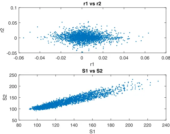
-0.06 -0.04 -0.02 0 0.02 0.04 0.06 0.08
r1 -0.05
0 0.05 0.1
r2
r1 vs r2
80 100 120 140 160 180 200 220 240
S1 50
100 150 200 250
S2
S1 vs S2
is dependence as seen by a plot of the two stock prices against each other across a subsample of days and paths presented.
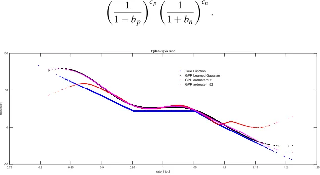
We now train a Gaussian process regression to learn the dependence of the change in the first stock price as a function of the ratio of the two prices, own to other on a subsample of days and paths. Figure3presents the result.
We see that a Gaussian process regression is capable of learning the existing dependence.
3.3 A two-dimensional analysis of pure discount bond data
We anticipate that bond prices of different maturities must be dependent but may also have no covariation if they are pure jump processes moving at their own times that are not synchronized across the maturity spectrum. The dependence comes from a possible dependence of drift via the dependence of parameters of motion on the prices themselves.
To investigate this further, daily time series of pure discount bonds were con-structed from data on yields to maturity each day for a variety of maturities. The data comes at specific maturities that vary each day. By interpolation, pure discount bond prices were derived for the fixed maturities of 1, 3, 6, 9, and 12 months and 2, 5, 10, 15, and 20 years . The data set went from January 3, 2007, to August 29, 2017, for 2782 days. Beginning on December 19, 2007, and employing on a rolling basis of 252 days of past returns on each of the 10 time series, bilateral gamma parame-ters of motion were estimated for the logarithm of the pure discount bond prices (see the next section for further estimation details). One obtains as a result, 2530 sets of bilateral gamma parameters for each of the ten pure discount bonds.
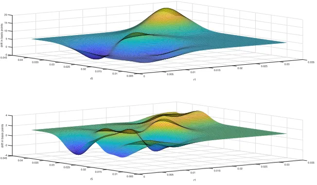
For an analysis of dependence, consider first just the dependence between the pure discount bond price for maturities of one and five years. From the bilateral gamma parameters we inferred for each day the expected exponential variation in the price as
1 1−bp
cp 1
1+bn
cn
.
0.75 0.8 0.85 0.9 0.95 1 1.05 1.1 1.15 1.2 1.25 ratio 1 to 2
-50 0 50 100
E[deltaS]
E[deltaS] vs ratio
True Function GPR Learned Gaussian GPR ardmatern32 GPR ardmaterm52
For the analysis of the possible nonlinear dependence of drifts on the two con-tinuously compounded rates for the one and five year maturities we estimated a support vector machine regression using a Gaussian kernel. Figure4and present the estimated drift response surfaces.
There is a sufficient nonlinearity in the drift response that creates potential depen-dence in the absence of any covariation as the processes remain independent bilateral gamma processes unless rates move to extreme regions. We observe that when rates are high the price drifts are positive indicating a drop in rates with the opposite occurring when rates are low.
4 Estimating exponential variations
The estimation of exponential variations daily is based on estimating the parameters of an uncentered distribution of returns that may be estimated from say 252 days of data on immediately prior continuously compounded returns. Critical to such an exer-cise is the choice of the parametric class of distributions. Clearly the class must be capable of fitting the data but hopefully not be so wide as to permit over fitting. The imposition of structural restrictions helps to reduce parameters and simultaneously avoid over fitting. On the other hand some parametric richness helps in differentiat-ing possibilities away from imposdifferentiat-ing too many symmetries. In this regard we rely on experience in fitting return distributions both risk neutrally and in the time series data.
The theoretical structural restriction is to appeal to a limit law for the distribu-tion. This is on the grounds that the number of price moves involved in the unit time
-5 0.045 0
0.04 5
0.035 0.035
drift in basis points
0.03 10
0.03
0.025 r5
0.025 15
0.02 r1
0.02 20
0.015 0.015 0.01 0.005 0.01
0.005 0
-4 0.045 -2
0.04
0.035 0.035
0
drift in basis points
0.03
0.03 0.025
r5 2
0.025
0.02 r1
0.02 4
0.015 0.015 0.01 0.005 0 0.005 0.01
of a day, though finite, is quite large. The limit laws arise at infinitely many moves and have been characterized as the self decomposable laws by L´evy (1937) and Khintchine (1938). They are a subclass of the infinitely divisible distributions with a further restriction on the associated L´evy density. Arrival rates of jumps when scaled by the absolute jump size must be decreasing functions of the absolute jump size (Sato (1999)). The self decomposable laws also have provably unimodal distributions and thereby refrain from overfitting a multiple of modes.
There are asymmetries between the way market prices rise and how they fall. It is often said that markets take the escalator up and the elevator down. Recently these differences were explored and documented in Madan and Wang (2017), and Madan, Schoutens and Wang (2017). Further, appealing to price moves being surprises occur-ring at surprise times modeled by Poisson arrival times for fixed jump sizes, we employ a pure jump price process. Thus we refrain from employing a continuous component either deterministic or random in the price process or its logarithm. The random continuous processes impose a symmetry between the upward and downward motion and do not permit a split between the two. They are also processes of infinite variation that do not permit the two processes of upward and downward motion to be separated. Already the use of limit laws stretches reality by allowing for infinitely many moves. Infinite variation is yet another stretch away from reality.
A particularly simple pure jump process with a self decomposable law at unit time is given by the variance gamma model of Madan and Seneta (1990) and Madan, Carr and Chang (1998). The jump arrival rate function when scaled by the absolute jump size is just a negative exponential of the absolute jump size, a clearly decreas-ing positive function. It permits a separation of the upward and downward motion, with both processes being gamma processes with separate scale parameters and the same shape or speed parameters. Madan and Wang (2017), Madan, Schoutens and Wang (2017) document that identical speeds on the two sides may be overly restric-tive and they employ the bilateral gamma process of K¨uchler and Tappe (2008). This is a difference of two gamma processes with their own speed and scale parameters. It is observed that the upward motion has a higher speed and lower scale parameter when compared to the same for the downward motion. Other asymmetric construc-tions of price motion could also be employed by entertaining the differences of other subordinators.
The estimation is conducted to match by weighted least squares the bilateral gamma model tail probabilities to their observed counterparts. The data on daily returns is sorted in increasing order and pointskiare extracted by interpolation of the
empirical distribution function such that the probability of returns being less thanki
isi/100 fori=1,· · ·,99. The observed tail probabilities are
yi=
i
1001ki<0+
1− i 100
1ki>0.
For the model probabilities with scale and speed parameters bp, cp and bn, cn
Eexp(iuX)=
1 1−iubp
cp 1
1+iubn
cn
.
The bilateral gamma process is given in terms of two independent standard gamma processesγp, γnby
X(t)=bpγp(cpt)−bnγn(cnt).
The density may be obtained by Fourier inversion of the characteristic function. Starting values are derived from an estimation of the variance gamma process that is a special case of the bilateral gamma withcp=cn =C. The variance gamma arrival
rate function (Madan and Seneta (1990), Carr, Geman, Madan, and Yor (2002)) has the form
kV G(x)=
C
|x|(exp(−Mx)1x>0+exp(−G|x|)1x<0) (1)
andbp = 1/M, bn = 1/G. The closed form for the variance gamma density
(Carr and Madan (2014)) is
fV G(x)=
(GM)C
2C−1(C)√2πG+M 2
C−1/2
exp
G−M
2 x
|x|C−1/2KC−1/2
G+M
2 |x|
,
whereKν(x)is the modified Bessel function andC, G, M are the variance gamma
parameters associated with its arrival rate function (1). The variance gamma density is used to estimate variance gamma tail probabilities to first fit the variance gamma model to observed tail probabilities to get starting points for the bilateral gamma estimation. In both cases, withyibeing the model tail probability the weighted least
squares optimization criterion employs the Andersen and Darling (1952) weights to minimize
z=
i
(yi−yi)2
yi(1−yi)
.
Once the parameters have been estimated the exponential variation for the day in basis points is given by
η=10000
1 1−bp
cp 1
1+bn
cn
−1
.
For all the underlying assets, time series of exponential variationsηmtare constructed
for assetmon dayt. Also employed are the time series of pricespm,t for the price
of assetmon dayt. The collection of variations and price histories are the inputs for support vector machine nonlinear regressions designed to learn how the variations depend on the prices.
5 Economic cost of exposure to model residuals
much larger base set of transforms. The parameter estimation algorithms employ reg-ularization tradeoffs and numerous fit statistics for determining the selected predictor. We then seek a uniform basis for comparing and contrasting the various predictors. One could use least squares, weighted least squares, or other weighted norms with related issues on specifying the weights to be employed. The possibilities are many and the principles to be used in formulating the final criterion quite unclear. In any case, the variety of goodness-of-fit criteria or distance metrics available generally pay little attention to economic matters and are directed towards statistical considerations like the ability to derive distributional properties in some stylized ideal environments. These statistical results enable one to assert that the observed improvement would have been unlikely to occur by chance and so it should be viewed as a significant improvement. Instead of judging improvements on such a statistical basis we ask if the improvement represents an economic advancement.
For the development of an economic assessment for a predictor we seek an answer in terms of the economic cost of the error or the residual. Consider then the perspec-tive for predicting a targetywith a predictionydelivered by some model. Suppose the target is a cash flow that we have to pay out. Further suppose we may arrange to receive the predictiony. In the absence of a prediction we make no such arrangement and theny = 0. The random net position is theny−yand we recognize that it is unlikely to be zero.
Now, under the traditional law of one price, all risky positions are worth what one could buy or sell them for as one can always trade in both directions at the same price. If you buy something for a price it is worth that price and you receive a value equal to what you paid for it. Similarly, if you sell something for a price the value delivered equals the price. There are no costs associated with risky positions. However, economic analysis may be conducted on replacing the fiction of the law of one price by that of a two price economy where it is recognized that prices for trading with the market depend on the direction of trade and you have to buy at higher prices than what you can sell for. You do not receive an equal value and the cost of a risky position may be modeled by the spread between the upper and lower valuations. The economic cost of prediction errors may then be taken to be this spread. Importantly, it is useful to note that economic costs are invariant to perturbation by constants as they affect both the upper and lower valuations equally.
lowering lower tail probabilities for the upper valuation. The resulting expectations may also be seen as Choquet (1953) expectations with respect to nonadditive proba-bilities. Here, we evaluate the economic cost of prediction errors using such distorted expectations.
The concave distortion used for the lower valuation, termed minmaxvar, was introduced in Cherny and Madan (2009) and is given by the parametric form
(u)=1−1−u1+1γ
1+γ
.
Other well known distortions from the insurance literature include the Wang (2000) transform. The greater the value ofγ, the more concave the distortion with no distor-tion occurring atγ =0. The set of test probabilities approving risk acceptability are all alternative probabilitiesQsatisfying
Q(A)≤ (P (A)) ,for all setsA,
whereP is the original or true physical probability (Madan, Pistorius, and Stadje (2017)). The upper valuation may be obtained using the complementary distortion
(u)=1−(1−u).
The value of distortion parameterγemployed in our calculations of economic cost is 0.75 as hedge fund returns are just acceptable at such a level as reported in Eberlein and Madan (2009). Hence, such a distortion is sufficiently conservative.
By way of an example, we note that the percentage reductions in economic cost delivered by least squares and support vector machine regressions in explaining the exponential variations for the prices of one-year pure discount bonds, using as explanatory variables the one and five-year rates, are 6.12 and 15.88%, respectively. The corresponding values for the five-year pure discount bonds are 7.12 and 38.39%. Though the absolute levels of economic cost vary and rise with the chosen stress level
γ, the percentage reductions rendered by models are comparable across a wide range of such levels.
6 Bivariate examples of zero covariation dependence
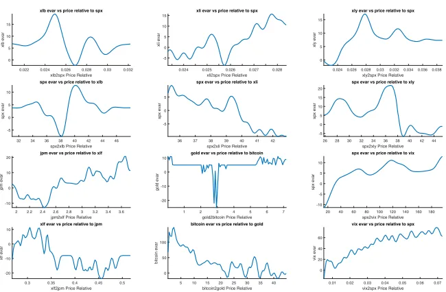
This section presents results on rsvm regressions of exponential variations of assets on the ratio of its price to that of a benchmark asset. Also presented are results of rsvm regressions of exponential variations on the own price and the benchmark price taken separately. Let us first consider sector ETF’s relative to the S&P 500 index and the index response to the sector ETF. Table1report the percentage reductions in economic exposure costs attained by linear and rsvm regressions of exponential variations of the ETF’s and the SPX, respectively, on the ratio and the two prices separately. We see considerable cost savings related to using the prices separately as opposed to the ratio though results for the latter may be more easily graphed.
Table 1 The first four columns present the reduction in economic cost achieved in explaining exponential variations in the levels of the ETF’s
Economic cost reductions in explaining Economic cost reductions in explaining exponential variations of ETF’s exponential variations of SPX Numerator Linear ratio to SPX Linear plus SPX rsvm ratio to SPX rsvm plus SPX Linear ratio Linear vector rsvm ratio rsvm vector
XLB 0.0258 0.2144 0.0383 0.3810 0.0070 0.1626 0.0099 0.3389
XLE 0.0518 0.2123 0.0335 0.3524 0.0015 0.1209 0.0708 0.3327
XLF 0.0248 0.1060 0.2361 0.3363 0.0064 0.0502 0.0510 0.2827
XLI 0.1772 0.1298 0.1187 0.3645 0.1277 0.1010 0.0968 0.3205
XLK 0.0788 0.0539 0.0823 0.3788 0.0269 0.0483 0.0781 0.2928
XLP 0.0212 0.0320 0.0002 0.0515 0.0555 0.0818 0.1153 0.3746
XLU 0.0985 0.1970 0.0026 0.1405 0.1331 0.0844 0.2153 0.2949
XLV 0.0026 0.1199 0.0355 0.2565 0.0022 0.1505 0.0497 0.3636
XLY 0.0979 0.0286 0.2210 0.2233 0.0903 0.0551 0.2754 0.3465
The variables used are the ratio of price to spx (S&P 500 index) and the two variables separately. Prediction is by linear regression or support vector machine regression. The last four columns switch to explaining exponential variations in the level of the spx index using the ratio to the ETF and the two variates of the ETF and the spx index separately
0.022 0.024 0.026 0.028 0.03 0.032 xlb2spx Price Relative 0
5 10 15
xlb evar
xlb evar vs price relative to spx
0.024 0.025 0.026 0.027 0.028 xli2spx Price Relative -5 0 5 10 15 xli evar
xli evar vs price relative to spx
0.0240.0260.028 0.03 0.0320.0340.0360.038 xly2spx Price Relative 0
5 10 15
xly evar
xly evar vs price relative to spx
32 34 36 38 40 42 44 46 spx2xlb Price Relative -5
0 5 10
spx evar
spx evar vs price relative to xlb
36 37 38 39 40 41 42 spx2xli Price Relative -5
0 5
spx evar
spx evar vs price relative to xli
26 28 30 32 34 36 38 40 42 44 spx2xly Price Relative -5 0 5 10 15 20 spx evar
spx evar vs price relative to xly
2 2.2 2.4 2.6 2.8 3 3.2 3.4 3.6 jpm2xlf Price Relative -10
0 10 20
jpm evar
jpm evar vs price relative to xlf
1 2 3 4 5 6 7 gold2bitcoin Price Relative -20
-10 0 10
gold evar
gold evar vs price relative to bitcoin
20 40 60 80 100 120 140 160 180 spx2vix Price Relative -10 -5 0 5 10 spx evar
spx evar vs price relative to vix
0.3 0.35 0.4 0.45 0.5 xlf2jpm Price Relative -20
-10 0 10
xlf evar
xlf evar vs price relative to jpm
5 10 15 20 25 30 35 40 bitcoin2gold Price Relative 0
50 100
bitcoin evar
bitcoin evar vs price relative to gold
0.01 0.02 0.03 0.04 0.05 0.06 0.07 vix2spx Price Relative 0
20 40 60
vix evar
vix evar vs price relative to spx
where the relationship between two entities is symmetric by construction, nonlin-ear dependencies estimated by support vector machines can be asymmetric with the first responding to the second in a certain way while second responds to the first in different way or not at all.
When an increase in an asset price relative to a benchmark price is associated with an increase in the asset price’s drift then we have momentum upwards. Otherwise we have mean reversion upwards. Similarly a drop relative to a benchmark being related to a fall in the asset’s own drift reflects downward momentum and downward mean reversion otherwise. We observe that xlb mean reverts to the index but the index has momentum on both sides relative to xlb. xli is in a momentum state with respect to the spx on both sides while the latter mean reverts to these. spx mean reverts to xly while the latter is flat with respect to spx.
Other interesting bivariate examples also presented in Fig.5are JPM relative to XLF, gold relative to bitcoin, and the SPX relative to the VIX. We observe that JPM has momentum relative to XLF on both sides while XLF mean reverts to JPM. Bitcoin reverts to gold while the latter is flat with respect to the former. Finally, both the SPX and the VIX are in a state of momentum with respect to the other on both sides.
7 Portfolio theory for two assets with zero covariation
Given that exponential variations appear to vary in some interesting and rational ways with the price levels suggests that the bilateral gamma parameters must themselves be nonlinear functions of the prices. As all four parameters are required to be positive, we consider regressing their logarithms on the prices and, in fact, use the log prices. Anticipating nonlinearities, we apply support vector machine regressions for each of the four parameters to build their dependence on the vector of prices. In this section, we first consider just the case of two assets and take, for example, JPM and XLF. Synthesizing the parametric dependence then requires eight support vector machine regressions. For the two assets JPM and XLF, we performed an rsvm of the loga-rithms of the four parameters on the two prices. The economic cost reductions on the four parameters of scale and speed up and down on jpm were 45.35, 2.73, 33.53, and 2.17 percent, respectively. The corresponding values for xlf are 41.40, 14.25, 28.18, and 16.74 percent. We next take as starting values initial prices in the middle of the data range at 39.06 and 12.00 for JPM and XLF, respectively, to simulate a thousand paths of length 252 days for the two price processes with bilateral gamma returns reflecting the rsvm estimated dependence of both speed and scale parameters on the current level of the two prices. Figure6presents a graph of the thousand pairs of continuously compounded returns to year end.
-1.5 -1 -0.5 0 0.5 1 1.5 2 2.5 Return on JPM
-0.5 0 0.5 1 1.5 2
Return on XLF
rsvm estimated bilateral gamma Hunt process returns
Fig. 6 Simulated returns on JPM and XLF over a year from model allowing all four parameters of a local bilateral gamma evolution to depend on both prices using support vector machine regression parameter predictions that are then input into a bilateral gamma simulator
8 Multi asset portfolio construction
By way of an illustration, we consider the construction of a portfolio invested in the nine sector exchange traded funds and the S&P 500 index. First, we construct the time series of bilateral gamma parameters for all ten assets. This was done for each day from January 3, 2008, to February 16, 2017, for a total of 2298 days using for each day the immediately prior 252 daily returns. We then perform 40 support vector machine regressions for each of the four parameters for each of the ten assets onto the data on the current prices for all ten assets. Table2presents the resulting sample percentage reductions in economic residual exposure cost delivered by the support vector machine regressions. The reductions are over 70% for the set of scale parameters and generally well over 20% for the speed parameters.
0 0.1 0.2 0.3 0.4 0.5 0.6 0.7 0.8 0.9 1 proportion in jpm
1.14 1.16 1.18 1.2 1.22 1.24 1.26
Portfolio Value
Two Asset ZCP portfolio value
Fig. 7 The graph show the zero covariation portfolio value computed as a distorted expectation of port-folio returns when local parameters of bilateral gamma motion depend nonlinearly on the two prices. The nonlinear dependence is estimated using support vector machine regressions. The value is presented as a function of the Proportion invested in the stock JPM
Table 2 Presented are the percentage reductions in economic cost achieved by support vector machine regressions of each of four bilateral gamma parameters of motion on the set of all ten asset prices being used to form the portfolio
Economic cost reductions in explaining bilateral gamma parameter variations
Asset bp cp bn cn
XLB 0.7118 0.2730 0.6917 0.2373
XLE 0.7949 0.3700 0.8182 0.3712
XLF 0.8790 0.2651 0.8370 0.5581
XLI 0.7720 0.2388 0.7558 0.3569
XLK 0.8003 0.1720 0.7375 0.2468
XLP 0.5554 0.3532 0.6455 0.3757
XLU 0.7228 0.2954 0.7372 0.3354
XLV 0.6854 0.1767 0.6415 0.2234
XLY 0.8094 0.1730 0.7756 0.2469
The portfolio is selected to maximize a conservative lower price for the portfolio value with cash flow to portfolio weightsxgiven by
Cj(x)=
10
i=1
xiexp(Rij).
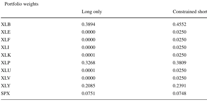
The portfolio objective is a conservative portfolio value calculated as a distorted expectation of the portfolio cash flows using minmaxvar at stress level 0.75. We solve for two portfolios, the first being long only while the second allows short posi-tions constrained to be above negative 2.5%. In each case the portfolio weights are constrained to sum to unity. The two sets of portfolio weights are presented in Table3. The long only portfolio invests inXLB,XLP,XLY, andSP X. The short con-strained portfolio increases the investment in the aforementioned assets and shorts the following at the maximum level:XLE,XLF,XLI,XLK,XLU, andXLV. Such a portfolio selection could be run regularly, say once a month and the portfolio rebal-anced to the new weights that are adapted to a current analysis of zero covariation dependence across the ten assets.
8.1 Rebalancing zero covariation dependence portfolios
We report here on applying conservative portfolio value maximization for portfolio selection with rebalancing every 21 days. The objective maximized is the distorted expectation of portfolio cash flows three months out after they are simulated by locally bilateral gamma processes reflecting parameter dependence on price levels. The dependence is calibrated by support vector machine regressions using the imme-diately prior 252 daily parameter values for dependent variables and the vector of contemporaneous prices as the independent variables. The number of shares held are
Table 3 The Table presents the portfolio weights attained by maximizing conservative portfolio values calculated as distorted expectations of portfolio returns for two portfolio selections
Portfolio weights
Long only Constrained short
XLB 0.3894 0.4552
XLE 0.0000 0.0250
XLF 0.0000 0.0250
XLI 0.0000 0.0250
XLK 0.0001 0.0250
XLP 0.3268 0.3809
XLU 0.0001 0.0250
XLV 0.0000 0.0250
XLY 0.2085 0.2391
SPX 0.0751 0.0748
constant between rebalancing dates. Figure8presents the daily mark-to-market value of the rebalancing portfolio strategy along with the prices of the component assets.
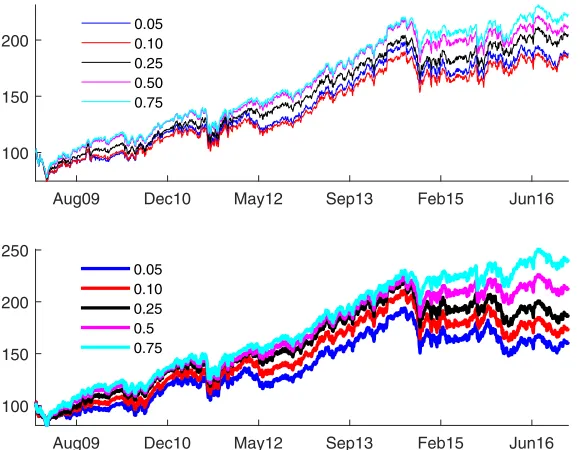
Figure 9 presents the mark-to-market value using different stress levels for portfolio selection for a long only strategy and a strategy constraining the short side to 2.5%.
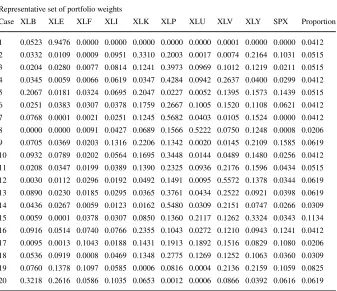
Table4presents a representative set of 20 portfolio weightings adopted over time along with the proportion of points they represent.
8.2 Comparison with Markowitz portfolio selection
This section reports on comparing the conservative portfolio value maximizing port-folio at stress level 0.75 and short position constraint of 2.5% with portfolios that are rebalanced along Markowitz lines. For a covariance matrixand mean return vector
μ, the Markowitz portfolio used is
x=
−1μ
1T−1μ.
However, as is well known, such portfolios can be quite unbalanced with large long and short positions that may even be totally unreasonable and impossible to hold or implement. To make them reasonable they were scaled to a volatility target of 20% with the rest of the funds held as cash. The covariance matrix was estimated from data on 252 immediately prior returns. For the mean returns we used first, the sample average over the past 252 days and second the exponential variation as estimated from the bilateral gamma process parameters.
6 1 n u J 5
1 b e F 3
1 p e S 2
1 y a M 0
1 c e D 9
0 g u A
Dates 50
100 150 200 250 300 350
Value
Monthly Rebalanced Portfolio vs Components
xlb xle xlf xli xlk xlp xlu xlv xly spx portfolio
Aug09 Dec10 May12 Sep13 Feb15 Jun16 100
150 200
0.05 0.10 0.25 0.50 0.75
Aug09 Dec10 May12 Sep13 Feb15 Jun16
100 150 200 250
0.05 0.10 0.25 0.5 0.75
Fig. 9 Mark to market values for long only strategy in the upper panel and long short with a short side constraint of 2.5% in the lower panel. The different curves represent different stress level used for the calculation of conservative portfolio vale as a distorted expectations of portfolio returns
Presented in Fig.10are the time paths of accumulated portfolio values starting with a 100 dollar investment, rebalanced monthly or every 21 days, using the three rebalancing portfolio selections.
We observe that the overall performance delivered by using sample averages for the mean returns is dominated by the use of mean returns extracted from distribution fitting. The conservative portfolio value maximizing portfolio delivers a smoother outcome with, an already observed, more stable set of portfolio weightings.
8.3 Performance statistics on randomly selected portfolios
Table 4 The Table shows a representative set of portfolio weights in the ten assets adopted at different points in time over the various rebalancings
Representative set of portfolio weights
Case XLB XLE XLF XLI XLK XLP XLU XLV XLY SPX Proportion
1 0.0523 0.9476 0.0000 0.0000 0.0000 0.0000 0.0000 0.0001 0.0000 0.0000 0.0412 2 0.0332 0.0109 0.0009 0.0951 0.3310 0.2003 0.0017 0.0074 0.2164 0.1031 0.0515 3 0.0204 0.0280 0.0077 0.0814 0.1241 0.3973 0.0969 0.1012 0.1219 0.0211 0.0515 4 0.0345 0.0059 0.0066 0.0619 0.0347 0.4284 0.0942 0.2637 0.0400 0.0299 0.0412 5 0.2067 0.0181 0.0324 0.0695 0.2047 0.0227 0.0052 0.1395 0.1573 0.1439 0.0515 6 0.0251 0.0383 0.0307 0.0378 0.1759 0.2667 0.1005 0.1520 0.1108 0.0621 0.0412 7 0.0768 0.0001 0.0021 0.0251 0.1245 0.5682 0.0403 0.0105 0.1524 0.0000 0.0412 8 0.0000 0.0000 0.0091 0.0427 0.0689 0.1566 0.5222 0.0750 0.1248 0.0008 0.0206 9 0.0705 0.0369 0.0203 0.1316 0.2206 0.1342 0.0020 0.0145 0.2109 0.1585 0.0619 10 0.0932 0.0789 0.0202 0.0564 0.1695 0.3448 0.0144 0.0489 0.1480 0.0256 0.0412 11 0.0208 0.0347 0.0199 0.0389 0.1390 0.2325 0.0936 0.2176 0.1596 0.0434 0.0515 12 0.0030 0.0112 0.0296 0.0192 0.0492 0.1491 0.0095 0.5572 0.1378 0.0344 0.0619 13 0.0890 0.0230 0.0185 0.0295 0.0365 0.3761 0.0434 0.2522 0.0921 0.0398 0.0619 14 0.0436 0.0267 0.0059 0.0123 0.0162 0.5480 0.0309 0.2151 0.0747 0.0266 0.0309 15 0.0059 0.0001 0.0378 0.0307 0.0850 0.1360 0.2117 0.1262 0.3324 0.0343 0.1134 16 0.0916 0.0514 0.0740 0.0766 0.2355 0.1043 0.0272 0.1210 0.0943 0.1241 0.0412 17 0.0095 0.0013 0.1043 0.0188 0.1431 0.1913 0.1892 0.1516 0.0829 0.1080 0.0206 18 0.0536 0.0919 0.0008 0.0469 0.1348 0.2775 0.1269 0.1252 0.1063 0.0360 0.0309 19 0.0760 0.1378 0.1097 0.0585 0.0006 0.0816 0.0004 0.2136 0.2159 0.1059 0.0825 20 0.3218 0.2616 0.0586 0.1035 0.0653 0.0012 0.0006 0.0866 0.0392 0.0616 0.0619 Also presented in the final column are the proportion of rebalancings represented by the portfolio weightings in that row
6 1 n u J 5
1 b e F 3
1 p e S 2
1 y a M 0
1 c e D 9
0 g u A
Dates
100 120 140 160 180 200 220 240 260
Mark to Market Values
Max Short 2.5%
Stress 0.75 Max Short 2.5 Bid Maximization MV sample average
MV BG Evar
Table 5 The Table presents percentiles of ten performance statistics for three investment strategies Performance statistics
Percentile ZCP MVA MVBGEV Percentile ZCP MVA MVBGEV
Total returns Sharpe ratios
5 193.2717 68.9452 76.7186 5 0.4656 0.1947 0.2326
25 255.4264 120.9758 127.8869 25 0.6057 0.2951 0.3367
50 306.5203 161.9877 174.9696 50 0.6931 0.3797 0.4392
75 367.5754 233.1460 258.1319 75 0.7969 0.5046 0.5674
95 493.4716 444.3992 454.0174 95 0.9288 0.7307 0.7309
Gain loss ratios Proportion positive
5 1.1344 1.0667 1.0875 5 0.4541 0.4354 0.4392
25 1.1699 1.0880 1.1091 25 0.4601 0.4433 0.4475
50 1.1928 1.1074 1.1334 50 0.4652 0.4506 0.4539
75 1.2257 1.1461 1.1665 75 0.4711 0.4550 0.4608
95 1.2504 1.2088 1.2028 95 0.4769 0.4656 0.4696
Acceptability index Max draw down
5 0.0225 0.0113 0.0146 5 35.9336 43.5110 39.9070
25 0.0282 0.0148 0.0179 25 50.1653 62.3000 49.4967
50 0.0318 0.0179 0.0215 50 60.4912 80.1955 64.5189
75 0.0365 0.0236 0.0268 75 71.4947 106.1338 94.8317
95 0.0400 0.0326 0.0314 95 114.6504 170.1741 149.8968
Skewness Kurtosis
5 7.0578 5.4547 6.2779 5 183.2202 150.5144 160.6891
25 11.4880 11.7356 12.6388 25 349.2345 370.6285 394.1370
50 15.0425 16.6281 20.6671 50 493.9739 558.1219 751.9566
75 18.6804 23.0900 26.7035 75 658.1477 868.8013 1053.7356
95 23.6825 29.3793 34.2800 95 900.6095 1194.4466 1464.7390
Peakedness Tailweightedness
5 0.8146 0.8313 0.8322 5 0.0106 0.0062 0.0029
25 0.8386 0.8598 0.8611 25 0.0159 0.0119 0.0095
50 0.8600 0.8781 0.8953 50 0.0220 0.0194 0.0159
75 0.8807 0.9039 0.9213 75 0.0282 0.0287 0.0276
95 0.9030 0.9387 0.9625 95 0.0342 0.0417 0.0406
They are zero covariation (ZCP) returns modeling with local bilateral gamma parameters of motion depending nonlinearly on all ten asset prices. Support vector machine regressions estimate the dependence. Also shown are mean variance portfolio selection with sample averages for means (MVA) and bilateral gamma exponential variations for the means (MVBGEV)
9 Conclusion
that covariances can arise at specific horizons only if integrated variations are stochastic. This observation suggests that perhaps variations are Markovian and func-tionally dependent on the price processes themselves. Anticipating the absence of such dependence except when price relativities are strained leads to the conjecture that the dependencies must be nonlinear. For stylized models with a known nonlin-ear dependence, it is verified that support vector machine regressions are capable of detecting the prevailing nonlinearity. For variations to depend on prices, the param-eters of the underlying bilateral gamma process should depend on prices. Support vector machine regressions are then employed to model parameter variations as depending nonlinearly on prices.
Given the complexity of support vector machine regression outputs, we seek statis-tics that capture the level of improvement delivered by such models. Model residuals are seen as liabilities to be paid out that have a conservative value when seen as an asset. This leads to employing the difference between the upper valuation for the residual less the lower valuation as a measure of the economic cost of holding the residual. Percentage reductions in economic costs of residuals then provide an assessment of model quality.
Once parameter dependence on prices has been synthesized using support vec-tor machine regressions, path spaces may be simulated to form multi asset return outcomes at an investment horizon. These are then used to form optimal portfolios that maximize a conservative or lower valuation maximizing portfolio value. Such an objective is an application of conic portfolio theory as set out in Madan (2016). Results are presented for monthly rebalanced portfolios over a period of nine years. The implementation of monthly rebalancing over nine years on a hundred randomly selected sets of ten equity underliers shows considerable improvements in vari-ous portfolio performance measures using lower price maximizing zero covariation portfolios over Markowitz portfolio selections with volatility targets.
Authors’ contributions
Both authors contributed equally to all aspects of the paper. Both authors read and approved the final manuscript.
Competing interests
Both authors indicate that they have no competing interests with respect to this publication.
References
Akaike, H: Information theory and an extension of the maximum likelihood principle. In: Petrov, BN, Cs´aki, F (eds.) 2nd International Symposium on Information Theory, Tsahkasdor, Armenia, USSR, September 2-8, 1971, pp. 267-281. Akad´emiai Kiad´o, Budapest (1973)
Andersen, TW, Darling, DA: Asymptotic Theory of Certain “Goodness of Fit” Criteria Based on Stochastic Processes. Ann. Math. Stat.23, 193–212 (1952).https://doi.org/10.1214/aoms/1177729437 Barndorff-Nielsen, OE, Shephard, N: Econometric Analysis of Realized Covariation: High Frequency
Based Covariance, Regression and Correlation. Econometrica.72, 885–925 (2004)
Bonanno, G, Lillo, F, Mantegna, RN: High-frequency Cross-correlation in a Set of Stocks. Quant. Finan.
1, 96–104 (2001)
Buchmann, B, Madan, DB, Lu, K: Weak Subordination of Multivariate Lavy Processes. Research School of Finance, Actuarial Studies and Statistics, Australian National University, Canberra (2016) Carr, P, Geman, H, Madan, D, Yor, M: The Fine Structure of Asset Returns: An Empirical Investigation.
J. Bus.75, 305–332 (2002)
Carr, P, Madan, DB: Joint Modeling of VIX and SPX options at a single and common maturity with risk management applications. IIE Trans.46, 1125–1131 (2014)
Carr, P, Wu, L: Time-Changes L´evy processes and option pricing. J. Finan. Econ.71, 113–141 (2004) Cherny, A, Madan, DB: New Measures for Performance Evaluation. Rev. Finan. Stud.22, 2571–2606
(2009)
Cherny, A: Markets as a Counterparty: An Introduction to Conic Finance. Int. J. Theor. Appl. Finan.13, 1149–1177 (2010)
Choquet, G: Theory of Capacities. Ann. de l’Institut Fourier.5, 131-295 (1953)
Eberlein, E, Madan, DB: Hedge Fund Performance: Sources and Measures. Int. J. Theor. Appl. Finan.12, 267–282 (2009)
Elliott, RJ, Chan, L, Siu, TK: Option Pricing and Esscher transform under regime switching. Ann. Finan.
4, 423–432 (2005)
Elliott, RJ, Osakwe, CJU: Option pricing for pure jump processes with Markov switching compensators. Finan. Stochast, 10 (2006).https://doi.org/10.1007/s00780-006-0004-6
Epps, TW: Comovements in Stock Prices in the Very Short Run. J. Am. Stat. Assoc.74, 291–298 (1979) Fasshauer, G, McCourt, M: Kernel Based Approximation Methods using Matlab. World Scientific,
Singapore (2015)
Kallsen, J, Tankov, P: Characterization of dependence of multidimensional L´evy processes using L´evy copulas. J. Multivar. Anal.97, 1551–1572 (2006)
Gerber, HU, Shiu, ESW: Option Pricing By Esscher Transforms. Trans. Soc. Actuaries.46, 99–191 (1994) Khintchine, AY: Limit laws of sums of independent random variables. ONTI, Moscow, Russian (1938) K¨uchler, U, Tappe, S: Bilateral Gamma Distributions and Processes in Financial Mathematics. Stoch.
Process. Appl.118, 261-283 (2008)
Luciano, E, Semeraro, P: Multivariate Time Changes for L´evy asset models: Characterization and Calibration. J. Comput. Appl. Math.233, 1937–1953 (2010)
L´evy, P: Th´eorie de l’Addition des Variables Al´eatoires. Gauthier-Villars, Paris (1937)
Madan, DB: A two price theory of financial equilibrium with risk management implications. Ann. Finan.
8, 489-505 (2012)
Madan, DB: Asset Pricing Theory for Two Price Economies. Ann. Finan.11, 1–35 (2015)
Madan, DB: Conic Portfolio Theor. Int. J. Theor. Appl. Finan.19(2016). available athttps://doi.org/10. 1142/S0219024916500199
Madan, DB: Measure distorted arrival rate risks and their rewards. Probability, Uncertainty and Quantita-tive Risk.2:8(2017a).https://doi.org/10.1186/s41546-017-0021-8.http://rdcu.be/tHKu
Madan, DB: Instantaneous Portfolio Theory (2017b). available athttps://ssrn.com/abstract=2804718 Madan, DB: Efficient estimation of expected stock returns. Finan. Res. Lett (2017c). available athttps://
doi.org/10.1016/j.frl.2017.08.001
Madan, D, Carr, P, Chang, E: The variance gamma process and option pricing. Rev. Finan.2, 79–105 (1998)
Madan, DB, Pistorius, M, Stadje, M: On Dynamic Spectral Risk Measures and a Limit Theorem. Finan. Stochast.21, 1073–1102 (2017).https://doi.org/10.1007/s00780-017-0339-1
Madan, DB, Schoutens, W: Conic Asset Pricing and the Costs of Price Fluctuations (2017). available at https://ssrn.com/abstract=2921365
Madan, DB, Schoutens, W: Applied Conic Finance, Cambridge University Press. UK, Cambridge (2016) Madan, D, Seneta, E: The variance gamma (VG) model for share market returns. J. Bus.63, 511–524
(1990)
Madan, DB, Wang, K: Asymmetries in Financial Markets. forthcoming Int. J. Financ. Eng (2017). available athttps://ssrn.com/abstract=2942990
Madan, DB, Schoutens W, Wang, K: Measuring and Monitoring the Efficiency of Markets (2017). available athttps://ssrn.com/abstract=2989801
Sato, K: L´evy processes and Infinitely Divisible Distributions. Cambridge University Press, Cambridge (1999)