R E S E A R C H
Open Access
Data-driven inference for stationary
jump-diffusion processes with application to
membrane voltage fluctuations in pyramidal
neurons
Alexandre Melanson
1,2*and André Longtin
1,3,4*Correspondence:
1Department of Physics, University
of Ottawa, Ottawa, Canada 2Département de physique et
d’astronomie, Université de Moncton, Moncton, Canada Full list of author information is available at the end of the article
Abstract
The emergent activity of biological systems can often be represented as
low-dimensional, Langevin-type stochastic differential equations. In certain systems, however, large and abrupt events occur and violate the assumptions of this approach. We address this situation here by providing a novel method that reconstructs a jump-diffusion stochastic process based solely on the statistics of the original data. Our method assumes that these data are stationary, that diffusive noise is additive, and that jumps are Poisson. We use threshold-crossing of the increments to detect jumps in the time series. This is followed by an iterative scheme that compensates for the presence of diffusive fluctuations that are falsely detected as jumps. Our approach is based on probabilistic calculations associated with these fluctuations and on the use of the Fokker–Planck and the differential Chapman–Kolmogorov equations. After some validation cases, we apply this method to recordings of membrane noise in pyramidal neurons of the electrosensory lateral line lobe of weakly electric fish. These recordings display large, jump-like depolarization events that occur at random times, the biophysics of which is unknown. We find that some pyramidal cells increase their jump rate and noise intensity as the membrane potential approaches spike threshold, while their drift function and jump amplitude distribution remain unchanged. As our method is fully data-driven, it provides a valuable means to further investigate the functional role of these jump-like events without relying on unconstrained biophysical models.
Keywords: Stochastic differential equations; Jump-diffusion processes; Membrane noise; Channel noise; Electric fish; Pyramidal neurons; Fokker–Planck equation; Chapman–Kolmogorov equation
1 Introduction
Complex systems are ubiquitous in many areas of science, including biology, neuroscience, climatology, engineering, as well as in finance and social sciences [1,2]. The common feature uniting such vastly different systems is the nonlinear interaction between their nu-merous microscopic constituents. This collective activity leads to the emergence of scopic order that cannot be reduced to microscopic properties [3]. It is often these macro-scopic variables that can be measured experimentally, allowing the emergent dynamics of
the system to be captured by low-dimensional data sets. The search for a macroscopic-level representation of the system thus relies on extracting dynamical information from observed time series [4].
For some systems, the high-dimensional, microscopic degrees of freedom can be well approximated by simple stochastic fluctuations. These fluctuations often participate as dynamical noise in the macroscopic evolution of the system. The low-dimensional repre-sentation of the system’s dynamics can then be expressed as a stochastic dynamical sys-tem [5]. More specifically, the observed data are usually assumed to satisfy a Langevin-type stochastic differential equation (SDE). A common approach is to obtain the drift and diffusion functions of this equation by estimating the first and second Kramers–Moyal coefficient [6,7]. The resulting model is completely data-driven and captures the core phenomenology of the original data without relying on knowledge or assumptions about the microscopic constituents of the observed system. This approach has been successfully applied in a variety of contexts, ranging from neuronal dynamics [8–12], heart rate vari-ability [13,14], turbulence [15,16], calibration of optical tweezers [17], and others (see Ref. [5] for a review).
In all mentioned cases, however, the noise is assumed to be purely diffusive, i.e., random fluctuations with continuous sample paths. This description is incomplete if, in addition to diffusive fluctuations, large and abrupt events appear at random times throughout the time series. In this case, jump-diffusion stochastic processes provide a more appropriate frame-work to model these data. Jump-diffusion processes have been used in neuroscience as a model for the spatial [18–21] and temporal [22] organization of synaptic bombardment, in physics as a model for noise-driven transport in ratchet potentials [23–25], as well as in finance [26,27] and soil moisture dynamics [28]. The Langevin approach is likely to fail if the observed system exhibits jump-diffusion characteristics, such as skewed distributions and sudden large jumps. In such cases, and especially when the microscopic dynamics are unknown, extracting a phenomenological model from the experimental data would provide a valuable tool to probe the dynamics of the observed system, its interaction with other systems, and the interplay between diffusive and jump noise sources in shaping the observed behavior.
In this paper, we present a novel, data-driven inference method that fits a jump-diffusion SDE to experimental time series. By detecting jumps through threshold-crossing and by calculating the contribution of diffusive fluctuations that are falsely detected as jumps, we iteratively estimate the drift function, noise intensity, jump rate, and jump amplitude distribution. The result of this semi-parametric method is a jump-diffusion SDE that suc-cessfully fits the original data. Our method is applicable in cases where these data are stationary, with additive diffusive noise and Poisson jumps. Note that other studies have attempted to infer jump-diffusion dynamics from data, but they rely on assuming a para-metric form of the jump amplitude distribution [29–31], or consider only Lévy processes [32,33].
recordings contain sudden and unpredictable jump-like events that occur among more typical diffusive membrane noise. Although the exact biophysical origin of these fluctua-tions is unknown, we find that the recordings are well fitted by jump-diffusion processes. We evaluate goodness of fit quantitatively by comparing the observed and the estimated probability density functions (PDF) and power spectral densities (PSD). Interestingly, we find that some pyramidal cells increase their jump rate and noise intensity as the mem-brane potential approaches spike threshold, while their drift function and jump amplitude distribution remain unchanged.
In Sect.2, we present the various steps involved in the inference procedure, including the detection scheme, the calculation relating to false positive, and the iterative approach. In Sect.3, we validate this procedure against one pure diffusion and two jump-diffusion test cases, and then we apply it to neurophysiological recordings of membrane noise. This is followed by a discussion on the possible generalizations of our method and on future work with the experimental data (Sect.4).
2 Methods
2.1 Definitions and overview
Let{X(t)}represent data in the form of a stationary time series. In what follows,{X(t)} is obtained either from experimental observations or from numerical simulation. In ei-ther case, the situation of interest here is when{X(t)}exhibits both diffusive fluctuations and abrupt events (henceforth called jumps). From{X(t)}, our goal is then to fit a jump-diffusion SDE of the form
dY(t) =FY(t)dt+√2D dW(t) +dJ(t), (1)
whereFis the drift function,Dis the noise intensity, andW(t) is a Wiener process (i.e., Brownian motion). HereJ(t) is a compound Poisson process representing the jumps
J(t) =
Nλ(t)
i=0
Bi, (2)
whereNλ(t) is a Poisson point process with rateλ, and theBi’s are the independent and
identically distributed jump amplitudes drawn from a distributionQB. For a small enough
sampling interval, or time stept, jumps will occur with probabilityΓB≡λt.
Although the method developed herein is applicable to a wide array of experimental data types, we do, however, impose certain conditions on the underlying dynamical pro-cess. Notably, we limit our analysis to systems where the dynamics are stationary (in the strict sense), the diffusion noise is additive, the jumps have positive amplitudes (Bi> 0),
and where the Poisson rateλis constant in time and small enough so thatΓB1.
Further-more, we assume here thatFis continuous and that a single stable fixed point arises from the deterministic part of the dynamics, but our method could be generalized to multistable systems. Except for this restriction, we assume no particular shape for the drift function as long as it generates a stationary process. Finally, we assume that, on average, jump am-plitudes are greater than the typical magnitude of diffusive increments: E[Bi] > (2Dt)
1 2
by one order of magnitude of more.
of the time series. Note that the value oftis set from the experiments that produced the data, and so is not a variable we can control. For experimental data, however, it is possible that the Markov property breaks down on the timescale of individual observations [5], but we assume that, in that case, the time series can be downsampled to a timescale where the Markov property then holds.
Furthermore, in the cases considered below, jumps appear unambiguously in the data, and so a jump-diffusion approach is warranted. In situations where this is not the case, the presence of jumps can be assessed from the fourth-order Kramers–Moyal coefficient, which is non-vanishing for processes with discontinuities [31,34]. Lastly, note that we make no assumptions regarding the structure of the ACF of{X(t)}; we only assume sta-tionarity in these data. In fact, we compare the ACFs (and PSDs) of time series generated by the fitted SDE with those of the original data as a means of validating the inference procedure.
Below we develop a data-driven inference procedure that successfully generates the estimatesDˆ,λˆ, Fˆ, andQˆB, where the unknown functionsF andQB are estimated
non-parametrically. This inference procedure results in a fitted stochastic processY(t) that is an adequate model of the original data. In this sense, we implicitly assume that the data {X(t)}are sampled from a realization ofY(t). In our calculations, we thus associate the first-order equilibrium PDF ofY(t),PY, to the empirical PDF of{X(t)}(obtained by kernel
density estimation)PX.
Our approach is predicated on the detection of jumps in the data via the applica-tion of a threshold θ∗ > 0 on the increments X(t+t)≡ X(t +t) –X(t). This procedure creates a pool of detected jumps with various amplitudes. Let QC be the
empirical PDF estimated from these measured jump amplitudes. Also, let n be the total number of increments in the time series, and m be the number of increments whose value is greater than θ∗. We define the (overall) jump detection probability as
ΓC ≡Prob{detecting an increment larger thanθ∗across an intervalt}, which we
esti-mate from the data asΓC=mn.
An inherent challenge with this threshold-crossing approach is that, in addition to the true jumps generated by the compound Poisson process, we also unavoidably detect large diffusive fluctuations that are falsely identified as jumps, henceforth called false positives (FP; Fig.1, top). A direct estimation of the true jump rateλand of the true jump amplitude distributionQBis thus impossible because the detected jump pool consists of a mixture of
true jumps and false positives. Our main contribution, and the central component of our inference procedure, is the calculation of FP-related statistics, namely the FP detection probabilityΓA≡Prob{detecting a diffusive increment larger thanθ∗across a given time
stept}and the distribution from which FP amplitudes are drawnQA. OnceΓAandQA
are calculated, we then extractλ(or, equivalently,ΓB) andQBfromΓCandQC. Note that
the subscripts “A”, “B”, and “C” will hereafter refer to FPs, true jumps, and both combined, respectively. More precisely, we measure quantities in “C” from the detected jump pool, we calculate FP statistics in “A”, and we seek the true jump statistics in “B”.
2.2 Choice of threshold
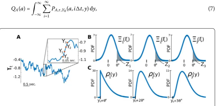
Figure 1Jumps are detected by applying a threshold on the increments,but this also creates false positives.Top: An example of a simulated jump-diffusion process where both true jumps (grey dots) and false positives (grey rings) are detected. The inset shows how the jump offset can be registered even if subsequent increments are positive.Bottom: Increment time series of the simulated process in the top panel. A jump is detected every time an increment exceeds the threshold. In this exaggerated case, true jumps are well above threshold, while false positives barely exceed it. This clear separation is not generally the case
Figure 2The choice ofθ∗is based on comparing the statistics of positive and negative increments. We show here how this strategy is applied to the two jump-diffusion validation cases presented in Sect.3.2. (A) The presence of true jumps allows the PDF of positive increments (blue histogram) to be differentiated from that of negative increments (red histogram) above a certain threshold (dashed line). (B) This threshold is chosen as the inflection point (red asterisks) of the difference between the sample means of the (truncated) positive and negative increments
be extracted from the statistical fluctuations ofQCandΓC. We thus aim for an
intermedi-ate value ofθ∗that captures most true jumps while allowing a manageable number of FPs. This is done by relying on our assumption of positive jump amplitudes and, more precisely, by exploiting the asymmetry between positive and negative increment statistics. Note that the threshold depends implicitly on the time step of the original time series: a smallert
means that diffusive fluctuations are smaller, and thus a smaller value ofθ∗can be used. Let{X+}and{X–}be the sets of positive and negative increments of{X(t)},
θ}be the reduced sets truncated byθ, whereθ spans the common range of{X+}and
{–X–}. We use the difference between the sample mean of these setsM+–M–as a
func-tion ofθ to quantify the relative importance of true jumps with respect to diffusive fluc-tuations, over different increment sizes. The value ofθfor whichM+–M–is a maximum
corresponds to the greatest separability between positive and negative increments. We find, however, that using the inflection point, i.e., where the second derivative becomes 0, located to the left of this maximum (Fig.2(B), asterisks) is a better choice of threshold. This slightly lower value retains a greater range of true jumps, which is desirable, while avoiding the inclusion of an overwhelmingly large number of FPs. Choosing this inflec-tion point rather than the maximum impacts primarily the estimainflec-tion ofλ, since it relies on the proper detection of true jumps in the time series. A slightly higher value ofθ∗will introduce a bias inλˆ. For instance, in the first jump-diffusion validation case that we con-sider in Sect.3.2, choosing the maximum as the threshold roughly yields a 1% increase in the error onλˆcompared to when the inflection point is used. Our approach for settingθ∗
is thus motivated by the fact that it is advantageous to choose a value as small as possible forθ∗, and the inflection point in the curve ofM+–M–provides a reliable way to achieve
this.
2.3 Jump detection
Here we describe how the threshold is applied to the increments in order to generate the detected jump pool. We apply a detection scheme tailored specifically to handle two aspects that we observe in experimental data with jumps, and it is inspired by the method used in [35]. Firstly, if the data are resolved on a fine enough time scale, jumps may last longer than a single sampling interval. Secondly, jumps need not be followed immediately by negative increments. In data, and in some simulations as well, the diffusive increments following a jump can still be positive, but we seek a method for identifying when the jump actually ends (Fig.1, inset). These two considerations shape the method used to calculate the FP amplitude distribution in Sect.2.4.2.
When a given increment is larger than the threshold, a jump onset timeTonis registered,
and if the next increment is below threshold, the associated offset timeToff is registered
(even if this increment is positive). This defines a jump of durationToff–Ton=t, where tis the sampling interval of the data. We henceforth refer to this type of jump as a sin-glet, as it spans the duration of a single time step. In contrast, if two or more successive increments are above threshold, then the jump is of duration 2tor more, which we refer to as a doublet, triplet, and so forth. In other words, the jump offset time is only registered at the end of the sequence of above-threshold increments. With the onset and offset times identified, a jump amplitude is defined as the difference betweenX(Toff) andX(Ton).
2.4 FP and true jump statistics
Here we present the calculations of the FP detection probabilityΓAand of the FP
ampli-tude distributionQA. We then show how these quantities are used to extract the true jump
rateλand the true jump amplitude distributionQBfrom the detected jump probabilityΓC
and the detected jump amplitude distributionQC. For the calculations in this subsection,
that the FP-related calculations involve only the diffusive part of Eq. (1) since, by defini-tion, FPs occur during the purely diffusive segments between true jumps. The calculations in Sects.2.4.1and2.4.2thus pertain only to diffusive incrementsYdiff(t). Finally, note that we perform validation tests of the calculations ofΓAandQAin Sect.3.1.
2.4.1 FP detection probability
As mentioned in Sect.2.1, sampling a jump-diffusion process such as Eq. (1) at finite in-tervals and applying a threshold on the observed increments leads to the detection of FPs, i.e., diffusive (rather than true jump) increments larger than the threshold. Importantly, these FPs occur with a probability that depends on the value of the process at the start of the interval. Let this conditional detection probability be defined as
α(y)≡Probdetecting an FP in the interval [t,t+t], given thatY(t) =y
=ProbYdiff(t+t) >θ∗|Y(t) =y. (3)
As α does not depend explicitly on time, this definition relies on our assumption that
Y(t) is stationary. They-dependence arises from the drift functionF. Indeed, if the drift function is positive (respectively, negative) at a given time, it biases diffusive fluctuations toward (away from) the threshold. This translates into an FP detection probability that assumes higher values whenF(y) > 0 than whenF(y) < 0. We now turn to the explicit calculation ofα(y).
LetΞY|Y(ξ|Y(t) =y) denote the PDF ofYdiff(t+t) conditioned on the value of the
process at the start of the interval, and whereξ assumes the possible values of the incre-ments. Note that, because the time step remains constant, it is always implied that the increments are defined across an intervalt. Given that we assumetto be sufficiently small, we approximateΞY|Yas the short-time propagator of the Fokker–Planck equation
[36,37] associated with the diffusive part of jump-diffusion process (recall that what con-cerns us here are the purely diffusive segments between the true jumps ofY(t)). We thus haveYdiff(t+t)≈N(F(Y(t))t, 2Dt) and
ΞY|Y
ξ|Y(t) =y≈√ 1
4πDtexp
–(ξ–F(y)t)
2
4Dt
, (4)
that is, a Gaussian distribution with meanF(y)tand variance 2Dt.
For the test cases presented in Sect. 3(witht= 10–4s), we have validated this
ap-proximation by comparing it with numerical solutions of the associated Fokker–Planck equation solved at a finer temporal resolution (t/1000) across the time stept. The nu-merical solutions were indeed well fitted with the approximation in Eq. (4) (not shown). Numerical integration was performed with a custom partial differential equation solver that implements a finite volume discretization along with the fully implicit Euler scheme. The advective term was treated with the upwind scheme, and a linear interpolation profile for the spatial derivative was applied to the diffusive term. The resulting algebraic equation was solved with the tridiagonal matrix algorithm [38].
Once the conditional PDF of the increments is evaluated with Eq. (4), we calculate the conditional FP detection probability, given that the process starts aty, as follows:
α(y) = ∞
θ∗
ΞY|Y
that is, the probability of observing an increment larger thanθ∗starting aty. Finally, the unconditional FP detection probability is calculated based on the empirical PDF of{X(t)},
PX:
ΓA=
∞
–∞
α(y)PX(y) dy. (6)
We validate these calculations in Sect.3.1.
2.4.2 FP amplitude distribution
We now proceed with the calculation ofQA, i.e., the distribution from which FP amplitudes
are drawn. First, recall that our detection scheme allows for jumps of different durations (Sect.2.3). As such, the detection of an FP implies either a succession of above-threshold increments (e.g., Fig.3(A)) or, at least, a single above-threshold increment. LetTFP
ondenote
the FP onset time, that is, the time at the start of the first above-threshold increment, and letY0≡Y(TonFP) be referred to as the starting value of the FP. Moreover, letτdenote the FP
duration, an integer multiple oft, such thatτ=tcorresponds to an FP singlet,τ= 2t
to an FP doublet, and so forth.
In order to calculateQA, let us first identify the factors that influence FP amplitudes.
Firstly, it must be noted that the FP amplitudes will exhibit a similary-dependence as that discussed in the preceding section. Indeed, an increment starting atY0≡Y(TonFP) =ywill
tend to be larger whenF(y) > 0 than whenF(y) < 0. Secondly, the amplitude of an FP will also depend on its duration,τ. For instance, the three increments of a triplet FP will sum-mate and tend to have a larger amplitude than that of a singlet. The FP amplitudesAwill thus covary withY0 and withτ, but note thatτ also depends onY0. Indeed, longer FPs
will tend to occur where the drift function is more positive, and vice versa. To account for these dependencies, let us define the trivariate random variable{A,τ,Y0}, distributed
ac-cording to its joint PDFPA,τ,Y0(a,it,y), where we explicitly writeτas an integer multiple
oft. What we seek then is the marginal:
QA(a) =
∞
–∞ ∞
i=1
PA,τ,Y0(a,it,y) dy, (7)
Figure 3The estimate of QAis obtained through a probabilistic analysis of FP detection. (A) Example of a diffusive
fluctuation registered as an FP triplet. (B) The situation in A is addressed by calculatingρi, the PDF ofYi
where the sum extends over all possible FP durations, and wherea> 0 represents all pos-sible amplitudes. From the definition of conditional PDFs, we can expand the joint PDF as follows:
PA,τ,Y0(a,it,y) =PA|τ,Y0(a|it,y)Pτ,Y0(it,y)
=PA|τ,Y0(a|it,y)Pτ|Y0(it|y)PY0(y), (8)
where Pτ|Y0(it|y) = Prob(detecting an FP of durationit, given the starting valuey) is
the conditional probability mass function of the FP durationτ. We can thus write Eq. (7) asa
QA(a) =
∞
–∞ ∞
i=1
PA|τ,Y0(a|it,y)Pτ|Y0(it|y)
PY0(y) dy. (9)
The sum in the large parentheses is a function ofy, and Eq. (9) is merely calculating its average with respect to the starting valueY0. This sum can further be interpreted as a
so-called mixture distribution: consider a collection of random variables, one of which is cho-sen according to a certain probability (itsmixture weight) and is then realized according to its own PDF (itsmixture component). The outcome of this experiment is itself a random variable whose PDF is called amixture distributionand is expressed as a sum over the PDFs of the random variables in the collection, weighted by their respective probabilities. In our case, for a fixed value ofY0, an FP duration is drawn according to a countable set
of mixture weightsPτ|Y0, and an FP amplitude is then realized according to the associated
mixture componentPA|τ,Y0. In practice, the sum will be truncated after the first few terms
because the subsequent mixture weights become negligible.
From Eq. (9), we see that in order to arrive at the desiredQA, the functionsPA|τ,Y0,Pτ|Y0,
andPY0must first be calculated. Let us first consider the latter. BecauseY0represents, by
definition, the value ofY(t) at the start of an above-threshold increment, we can express its PDF in terms of the joint PDF ofYdiff(t+t) andY(t):
PY0(y) =K
∞
θ∗
PY,Y(ξ,y) dξ
=K
∞
θ∗
ΞY|Y
ξ|Y(t) =yPY(y) dξ
=KPY(y)
∞
θ∗
ΞY|Y
ξ|Y(t) =ydξ
=KPX(y)α(y), (10)
whereKis a normalization constant and where, in the last line, we have replacedPY by
the empirical PDF of{X(t)}. Note that we integrate withθ∗as a lower bound in order to enforce thatY0is associated with the onset of an above-threshold increment. Let us now
consider the calculation ofPA|τ,Y0.
In what follows, we simplify the notation by labeling time with the indexi, such that
i= 0 represents the timeTonFP,i= 1 the timeTonFP+t,i= 2 the timeTonFP+ 2t, and so forth. With this notation,Yi≡Y(TonFP+it) denotes theith point following the FP onset
FPs of duration, sayit, which corresponds to a sequence ofisuccessive above-threshold increments. As such, the forthcoming calculations involve PDFs that are implicitly condi-tioned on the event{Ydiff
n >θ∗,∀n≤i}.
For an FP of durationτ=itstarting atY0, we define its amplitude asA=Yi–Y0, and
we seek the conditional PDFPA|τ,Y0. For this purpose, letρi(y)≡PYi|Y0(y|y0) denote the
PDF ofYi,i> 1, conditioned onY0. SinceAis expressed as the difference betweenYiand
Y0, we can directly write
PA|τ,Y0(a|it,y0) =ρi(a+y0). (11)
Theρi’s, fori> 1, are evaluated sequentially based on the fact thatYi=Yidiff+Yi–1. The
PDF of this sum, conditioned onY0, gives
ρi(y) =
∞
–∞PYi,Yi–1|Y0(
ξ,y–ξ|y0) dξ
= ∞
–∞PYi|Yi–1,Y0(ξ|y–ξ,y0)PYi–1|Y0(y–ξ|y0) dξ
= ∞
–∞
PYi|Yi–1(ξ|y–ξ)ρi–1(y–ξ) dξ. (12)
To enforce the condition of above-threshold increments,{Ydiff
n >θ∗,∀n≤i}, we evaluate
PYi|Yi–1based on Eq. (4), but we truncate the distribution belowξ=θ∗:
PYi|Yi–1(ξ|y) =K
⎧ ⎨ ⎩
ΞYi|Yi–1(ξ|Y(t) =y) ifξ>θ
∗,
0 otherwise, (13)
whereKis a normalization constant. With Eq. (13) and (12), we finalize the calculation of
PA|τ,Y0in Eq. (11). In Fig.3(B), we see the representation of theρifor an FP triplet. From
ρi, we can also calculate the PDF ofYidiff, conditioned onY0 (this will be useful in the
calculation ofPτ|Y0). Let this PDF be defined asΞi(ξ)≡PYi|Y0(ξ|y0). We calculate it as a
marginal overYi–1:
Ξi(ξ) =
∞
–∞
PYi,Yi–1|Y0(ξ,y|y0) dy
= ∞
–∞
ΞYi|Yi–1(ξ|y)ρi–1(y) dy, (14)
where the dependence ofΞYi|Yi–1onY0disappears because of the Markov property. In
Fig.3(C), we see the representation of theΞi’s for an FP triplet.
We now turn to the calculation ofPτ|Y0, the probability of observing an FP of duration
τ, conditioned on the starting valueY0. We are interested in the conditional probability of
the event{τ=it}, whereiis an integer. This event is equivalent to the intersection of the eventsE1≡ {Y1diff>θ∗},E2≡ {Y2diff>θ∗}, . . . andEi+1≡ {Yidiff+1 ≤θ∗}. In other words,
By successively applying the definition of conditional probability, we can expandPτ|Y0
as follows:
Pτ|Y0(it|y0) =Prob(τ=it|y0)
=Prob
Ei+1∩
i n=1 En y0 =Prob
Ei+1
i
n=1 En
,y0
·Prob Ei i–1 n=1 En ,y0
·Prob
Ei–1
i–2
n=1 En
,y0
·. . .·Prob(E2|E1,y0)·Prob(E1|y0).
LetZi(y0)≡Prob[Ei|(
i–1
n=1En),y0],i> 1, represent the probability that theith increment
is above threshold, given that thei– 1 previous increments were also above threshold, and given the starting valuey0. TheseZi’s can be calculated from theΞi’s of Eq. (14) as
(Fig.3(B), shaded area):
Zi(y0) =Prob
Yidiff>θ∗|Yndiff>θ∗,∀n<i;y0
= ∞
θ∗
Ξi(ξ) dξ. (15)
We now arrive at the desired probability mass function:
Pτ|Y0(it|y0) =Prob(τ=it|y0) =
1 –Zi+1(y0)
i
n=1
Zn(y0), (16)
where we have used the fact that 1 –Zi+1 is equal to the probability that the (i+ 1)th
increment is below threshold, and where we have definedZ1(y0)≡Prob(E1|y0) =α(y0),
i.e., the probability that the first increment afterY0is above threshold. Once Eq. (10), (11),
and (16) are evaluated, we apply Eq. (9) to obtain the desiredQA. Using this approach, we
obtain an excellent agreement between theory and simulations, as reported in Sect.3.1.
2.4.3 True jump rate
Our estimate of the true jump rateλrelies on the knowledge of the overall jump detection probabilityΓCand on the FP detection probabilityΓA(both defined in Sect.2.1). Recall
that we calculate ΓAfrom Eq. (6), while we estimateΓC directly from the data asm/n,
wheremis the number of time steps withX(t) >θ∗(either from a true jump or an FP) andnis the total number of time steps in the data time series. On the other hand, from the definition ofΓCwe can write:
ΓC≡Prob
detecting an increment larger thanθ∗across an intervalt
=Prob(detecting an FP acrosst)∪(detecting a true jump acrosst)
=ΓA+ΓB–ΓAΓB
whereΓB=λtis the probability of observing a true jump in an intervalt. This is merely
a statement of the addition law of probability, which would read: the probability of detect-ing a jump in an intervaltis the sum of the probability of observing a true jump, plus that of observing an FP, minus the probability of observing both at the same time, where we use the fact that FPs and true jumps are independent events. For the test cases described in Sect.3.2, isolatingλin Eq. (17) is accurate up to an error of 0.02%.
2.4.4 True jump amplitude distribution
As in the previous subsection, we obtain an estimate for the true jump amplitude distri-butionQBbased on the empirical PDF of jump amplitudes measured from the time series
QC and on the calculated FP amplitude distributionQA. Because detected jumps are a
mixture of true jumps and FPs, we can write, a priori,
QC=WAQA+WBQB, (18)
whereWA=ΓΓAC is the probability that a detected jump is an FP, andWB=
ΓB
ΓC that it is a
true jump. The subtlety here is that, contrary to FPs, true jumps are never detected on their own, as they always summate with a diffusive fluctuation. In other words, we never observe theBi’s directly, but rather theBi’s plus a diffusive increment. Over a short enough
time step, diffusive increments are Gaussian variables and are approximately independent of each other. For the purpose of calculatingQB, we will thus assume these increments are
Gaussian with mean zero and variance 2Dt. Properly accounting for they-dependence of the mean would be more precise, but would requireQCto be broken down into a family
of distributions parameterized byy, which would require a very large number of detected jumps in the data.
LetΞ˜ represent a Gaussian distribution with zero mean and variance 2Dt. TheQBin
Eq. (18) should thus be replaced by the convolutionΞ˜∗QB. Furthermore,WAmust in fact
be reduced by a factor (1 –ΓB) to account for the probability that FPs can occur during
the same interval as a true jump. This leads to
QC=
ΓA(1 –ΓB)
ΓC
QA+
ΓB
ΓC
(Ξ˜ ∗QB). (19)
From this equation, we isolate the convolution term and apply the basic deconvolution algorithm [39] to extractQB. Letfbe a measured, convolved signal, where the convolution
kernelhis known. We seek the intact signalg, such thatf = (h∗g). We compute an estimate ofgat each iteration asgk+1=gk+ [f– (h∗gk)], withg0=f. The algorithm converges once
the correct signal is reached, since the residual betweenf and (h∗gk) then becomes zero.
2.5 Iterative procedure, noise intensity, and drift function
We now turn to the problem of the simultaneous data-driven estimation of all the un-knowns in Eq. (1). To this end, we incorporate the calculations of Sect.2.4in the itera-tive scheme depicted in Fig.4, which consists of three main branches. The first two ini-tial branches, I and II, are independent and are performed only once; this is followed by branch III where the iterations take place. In branch I, the threshold is set (Sect.2.2) and then applied to the time series to yield the detected jump pool, from whichΓC andQC
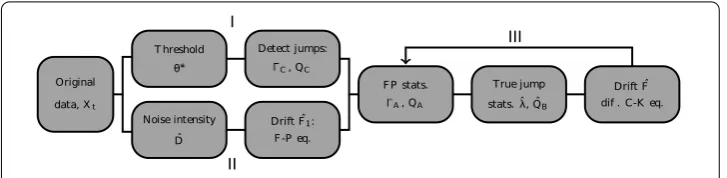
Figure 4Overview of the flow of our iterative procedure. In both validation cases, a satisfying estimate is obtained after about 10 iterations. The threshold and noise intensity are estimated directly from the data in I and II, while the true jump rate and amplitude distribution, as well as the drift function, appear in the iterative phase III. Note that the true jumps statistics are not yet established in II, and this is why we resort to the Fokker–Planck equation as a means to obtain a preliminary guess of the drift functionFˆ1. A more refined estimate ofFis later obtained at the end of branch III
guess for the drift functionFˆ1, which are both used in the first iteration of branch III to
calculateΓˆBandλˆ(Sect.2.4). The last step in branch III usesDˆ,ΓˆB, andλˆto estimate the
drift functionFˆ, which is fed back to the first step of branch III in order to iteratively refine the estimation procedure.
2.5.1 Noise intensity
As depicted in Fig.4, the estimation ofDdoes not rely on the value chosen forθ∗. It does, however, still use the notion of applying a threshold on the increments. Indeed, calculating
ˆ
Drelies on partitioning{X(t)}into mostly jump-free segments, the length and number of which is sensitive to the value of the threshold used for detection: the lower the threshold, the more jumps are detected (some of which are FPs) and the shorter these partitions are, which, as explained below, can skew the estimate ofD. A high threshold, on the other hand, leaves a significant number of true jumps in those segments. The goal here is thus to vary the thresholdθin order to obtain the optimal estimate ofD.
In the limit of an infinitesimally small sampling interval,t→0, the quadratic variation [Ydiff(t)] of a pure diffusion process converges to the so-called integrated variation, which,
for additive and time-independent noise, gives [40,41]
Ydiff(t)=
T
0
2Dds= 2DT, (20)
whereT= (n– 1)tis the total duration for thensamples of{X(t)}. We can, therefore, estimateDvia the sample quadratic variation, also known as realized variance,RV(t) [40, 41]:
ˆ
D≈ 1
2TRV(t) =
1 2T
n–1
k=0
Xdiff(tk+1) –Xdiff(tk)
2
. (21)
For instance, for a test diffusive process withF(y) = –0.2yandD= 0.15 and sampled at
Simply removing the detected jumps from the sum in Eq. (21) would, therefore, yield an underestimatedDˆ.
To circumvent this problem, we consider only the negative increments of{X(t)}in the calculation of Dˆ, as they will remain essentially unaffected by the presence of positive jumps, with the exception of a short transient following the jump offset. Indeed, following each jump, we expect to see a brief period where the process is out of equilibrium. And since the jumps have positive amplitudes, negative increment statistics are biased toward negative values during this transient (e.g., Fig.1). The calculation ofDˆis thus based on ap-plying Eq. (21) to jump-free segments of{X(t)}, but only including negative increments, and neglecting the initial transient at the start of each segment (the duration of which is determined below). This is repeated for various values ofθ. The successful estimation of
Dbased only on negative increments relies on our assumption thattis small, for in this case increments are approximately independent and distributed asN(0, 2Dt). For larger
t, the increment PDF can become asymmetric, meaning that the statistics of negative in-crements differ from those of positive ones, which would cause errors in our estimation ofD.
Let Toff andTon denote the jump offset and onset times, respectively. Note that the
values of these times and the number of detected jumps all depend on the specific value of the threshold. Then theith segment is defined by{S(t)}i={X(t) :Toff(i) <t<Ton(i+ 1)}
and is of durationTi=Ton(i+ 1) –Toff(i), and let{S(t)}ibe itsniincrements. Out of these
niincrements, we keep only then–i that are negative and that occur after the transient of
approximate durationΦ. We are thus left with the following subset of increments from each segment:
S(t)–i =S(t)i:S(t)i< 0,t>Φ. (22)
For each segment, we obtain an estimateDˆias follows:
ˆ
Di=
1 2T–
i n–
i
k=1
S(tk)
– i
2
, (23)
whereT–
i =n–itis the effective duration of the combinedn–i negative increments. We
then calculateDˆ as an average of theDˆi’s, weighted byTi/T.
More precisely, here are the steps taken in order to arrive atDˆ:
• Starting from the largest value of{X(t)}, lower the threshold until the largest 5% of jumps are detected, which are the ones with the most prominent transient.
• Let{S∗(t)}ibe the segments that follow these jumps (Fig.5(A)). Average across them
for each time step, creating a jump-triggered average trace (Fig.5(A)), black line). • IdentifyΦas the approximate moment when the jump-triggered average stabilizes,
quantified here as when its derivative is less than0.05(results do not depend strongly on this particular value: changingΦby one order of magnitude on either side of the value used here yields estimates ofDthat differ by less than 0.2%). This gives us an estimate for the maximum time scale required for post-jump equilibrium.
• WithΦdetermined, and for each value of the threshold, extract the{S(t)}i’s (Fig.5(B))
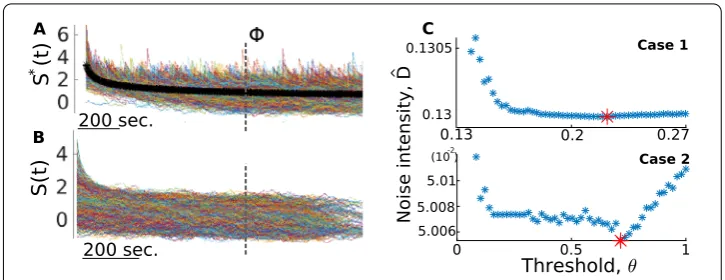
Figure 5CalculatingD relies on partitioningˆ {X(t)}in jump-free segments for different threshold values. We show here how this strategy is applied to the two jump-diffusion test cases presented in Sect.3.2. (A) A
jump-triggered average (black curve) is obtained from the largest 5% jumps in the data and is used to obtain a maximum estimate of the transient time scaleΦ(dashed line). (B) Jump-free segments used to calculated the optimal value ofDˆin C. (C) Different estimates ofDare produced for different values of the threshold. We heuristically choose the minimum value as the optimal value. Traces in A and B are from Case 2
This scheme results in an estimateDˆfor each value of the threshold, and the lowest value is chosen as the optimal estimate (Fig.5(C)). This is because this approach overestimates
Don both ends of the range of threshold values, but for different reasons. For lowθ, many more jumps are detected, and this makes the{S(t)}i’s shorter, which means that the
asso-ciatedDˆ is more prone to be biased by the residual of the transient. On the other hand, a very high threshold leaves significant jumps in the{S(t)}i’s, which biases the statistics of
negative increments. The optimal balance is reached somewhere in-between, where the segments are large enough so that the initial transient is negligible, and where the jumps that are inevitably left in the segments do not significantly alter the statistics of negative increments. The heuristic choice of an intermediate value, namely one that corresponds to the minimalDˆ estimate, gives excellent results in both validation cases (less than 0.1% error, see Table2).
2.5.2 Drift function
Our estimation of the drift functionF relies on the differential Chapman–Kolmogorov equation [42], which describes the evolution of the transition probability of a stochastic process where jumps occur alongside diffusive fluctuations. LetY(t) be a jump-diffusion process with transition probabilityPY|Y0. For the case of positive Poisson jumps and
ad-ditive diffusive noise, the differential Chapman–Kolmogorov equation reduces to (see the Appendix)
∂PY|Y0(y,t|y0,t0)
∂t = –
∂ ∂y
F(y)PY|Y0(y,t|y0,t0)
+D∂
2
∂y2PY|Y0(y,t|y0,t0)
–λPY|Y0(y,t|y0,t0) +λ
∞
0
QB(s)PY|Y0(y–s,t|y0,t0) ds. (24)
IfY(t) is assumed to have reached its equilibrium state, then the left-hand side vanishes, and in the right-hand side we can replace the transition probability with the first-order equilibrium PDF,PY,bwhich we assume to be equal to the empirical PDF,PX, of the
Note, however, thatFˆ is required in the first step of branch III of the iterative proce-dure (Fig.4), since the FP-related statistics,ΓAandQA, are calculated based on the drift
function. A preliminary estimateFˆ1of the drift function is thus required. This particular
estimate, which is needed only once throughout the inference procedure, is obtained by lettingλ= 0 in Eq. (24), such that it becomes the Fokker–Planck equation associated with the diffusive part of the stochastic process. The stationary solution of this Fokker–Planck equation can be used to establish a relation between the noise intensity, the drift function, andPY [37,43]:
PY(y) =
K
ˆ
Dexp
– Fˆ1(y) ˆ
D dy
, (25)
whereKis a normalization constant and where, again, we assume thatPY=PX. This first
preliminary estimate is necessarily flatter than the trueF, as the presence of jumps makes
PXwider than it would be if there were no jumps. Successive iterations gradually rectify
this by incorporating estimates ofλandQBin Eq. (24).
3 Results
Here we present three applications of the method developed above. First, we validate the calculation ofΓAandQAfor the case of a purely diffusive process. Then we apply the full
iterative scheme to two simulated jump-diffusion processes with different characteristics. Finally, we apply our inference method to electrophysiological recordings in pyramidal cells of electric fish.
3.1 Validation of the FP statistics calculations
To confirm that the calculations ofQAandΓAare accurate, we start with a simple test
case where we consider a time series{Xdiff(t)}obtained from a simulated pure diffusion process. As there are no jumps here, the distribution of increments does not possess the necessary asymmetry to properly identify a threshold. For this test case only, we thus opt for a specific value,θ∗= 0.1, that showcases the ability of our method to handle FPs of various durations. The results presented here, however, remain valid for a range of values ofθ∗. For the parameters used in this pure diffusion validation case (Table1), this range extends from 0.025 up to 0.2. The upper limit is set by the fact that, beyond it, too few FPs are detected, which precludes any statistical calculations from being achieved. The lower limit, on the other hand, arises because too many FPs are detected, such that, for instance, they occur every other time step. In such a case,tis too large and the estimation ofλ
becomes imprecise due to the statistical fluctuations in the number of detected FPs. Applying the threshold in this case leads to a detected jump pool comprised entirely of FPs. The goal now is to compare the measuredQCandΓCwith the calculatedQAandΓA.
If we obtain thatΓC≈ΓAand thatQC≈QA, then we will effectively have shown that the
true jump rate is zero,λ= 0, and that our method correctly calculates the FP amplitude distribution. In this pure diffusion test case, these calculations rely on the knowledge of the correct noise intensityDand the correct drift functionF, but this will not be the case in subsequent sections.
With the particular values ofDandFused here to simulate{Xdiff(t)}(Table1), we find
that FPs are either singlets, doublets, or triplets, which contribute differently to the mea-sured amplitude distributionQC. Indeed, the fact that longer FPs tend to have larger
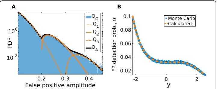
Figure 6For a pure diffusion process,we correctly calculate the FP amplitude distribution QAand FP detection
probabilityΓA. (A) After applying a threshold toXdiff(t), we obtain a pool of FPs with a range of durations
and amplitudes. From the latter we measureQC(blue histogram). We correctly calculate this distribution as
iQi, whereQiis defined in Eq. (26). (B) Probability of detecting an FP as a function ofy, calculated (yellow
curve) and Monte Carlo simulated (blue dots)
measured amplitude distribution (Fig.6(A), blue histogram). By taking the sum out of the integral in Eq. (9), we can writeQA(a) =∞i=1Qi(a), where
Qi(a) =
∞
–∞
PA|τ,Y0(a|it,y)Pτ|Y0(it|y)PY0(y) dy (26)
are the individual distributions associated with FPs of duration it (Fig. 6(A), yellow curves). These distributions are then summed to obtainQA, which is a precise match with
QCfor this purely diffusive example (Fig.6(A), black curve).
Furthermore, by applying Eq. (5) we calculate they-dependent detection probability,
α(y) (Fig.6(B), yellow curve). As expected, this function depends non-trivially onyand reflects the nonlinearity of the specific drift function used in this example. If multiplicative noise had been used, the noise intensity D(y) would also have influenced the shape of
α(y). To validate this calculation ofα(y), we run Monte Carlo simulations of the diffusion process
dYdiff(t) =FYdiff(t)dt+√2D dW(t), (27)
over a durationt, but with a time step oft/1000 and with various initial conditions along they-axis. For each initial condition, we evaluate the FP detection probability as the ratio between the number of Monte Carlo runs, whereYdiff(t) >Ydiff(0) +θ∗, and the total number of Monte Carlo runs (Fig.6(B), blue dots), the result of which precisely fits with the calculatedα(y). Finally, we obtain the overall FP detection probabilityΓAfrom
Eq. (6), which, in this pure diffusion test case, differs fromΓCby only 0.06%.
3.2 Validation of the iterative scheme
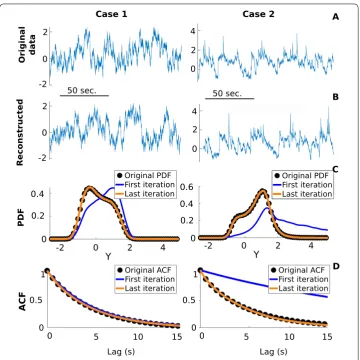
Figure 7Our inference method successfully fits a stochastic model to the original data. (A) Realizations of the jump-diffusion processes for the two different validation cases. (B) Simulation results from the jump-diffusion SDE inferred by our method. (C) Comparison between the PDF of the original validation data (black dots) and that of the last iteration of the fitted SDE (yellow curve). The PDF associated with the first iteration is also shown (blue curve). (D) Similar comparison between the original and estimated ACF
Case 2, where jumps are much larger than the background noise and their rate is double that of Case 1 (Fig.7(A)). The specific functions and parameters used to generate and analyze these validation data are shown in Table1, which can be summarized as follows: low rate, low amplitude, high noise for Case 1, and high rate, high amplitude, low noise for Case 2. Preliminary tests with a linear drift function showed a successful fit between the fitted SDE and the numerical data. We now opt for a more general and arbitrary shape where the drift function is nonlinear and non-monotonic. The only restrictions are that it yields a single stable fixed point and that the resulting stochastic process is stationary. We thus restrict our analyses to drift functions that are mostly decreasing. Although the parameters and functions used for the simulations are known, they are not used in the inference procedure, only{X(t)}is. To assess the performance of the proposed method, we compare the estimatedDˆ,λˆ,Fˆ, andQˆBwith their true values.
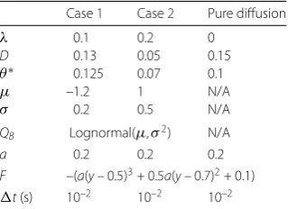
Table 1 Parameters and functions for the validation cases
Case 1 Case 2 Pure diffusion
λ 0.1 0.2 0
D 0.13 0.05 0.15
θ∗ 0.125 0.07 0.1
μ –1.2 1 N/A
σ 0.2 0.5 N/A
QB Lognormal(μ,σ2) N/A
a 0.2 0.2 0.2
F –(a(y– 0.5)3+ 0.5a(y– 0.7)2+ 0.1)
t(s) 10–2 10–2 10–2
amidst the FPs. In contrast, the jumps in Case 2 are well separated from the diffusive fluctuations, which allows for a more direct estimation ofQB. The presence of large jumps
in this case, however, significantly alters{X(t)}and its PDF, making it harder to estimateF. In both cases, however, we find that the original SDEs can be precisely recovered by our method. For instance, simulating Eq. (1) withDˆ,λˆ,Fˆ, andQˆBof the last iteration not only
produces time series that resemble the originals (Figs.7(A) and7(B)), but also yields an excellent fit between the reconstructed and original PDFs (Fig.7(C))), with anO(10–4)
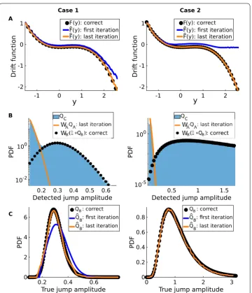
root-mean-square error (normalized by the range of{X(t)}) and ACFs (Fig.7(D)). Inspecting the results from the last iteration, we indeed see that the correct drift func-tion is recovered (Fig. 8(A)). This is done through the use of the so-called differential Chapman–Kolmogorov equation. This is then used to calculate the next QA and ΓA
(Fig.8(B)), which allows the correctQBto be demixed from the measuredQC(Fig.8(C)).
We also obtain low relative errors when comparing our estimates and the correct values of
Dandλ(Table2). Note also that, although not shown here, we obtain the same fit quality between original and reconstructed when we apply our method to hybrid cases, where, for instance, the small jump amplitudes are paired with a higher rate instead of a lower one and vice-versa.
3.3 Application to experimental data
Figure 8Our inference procedure recovers the correct parameters and functions from Eq.(1). (A) The correct drift function (black dots) is recovered in the last iteration (yellow curve). First iteration results are shown for comparison (blue curves). (B) We see that the measured amplitude distributionQCis in fact a mixture ofQA
(yellow curve) andΞ˜∗QB(black dots, see Eq. (19)). (C) After deconvolving the latter, we do recover the
correctQB(yellow curve). Note that in Case 2, the first and last iterations are confounded, as the true jump
amplitudes are almost directly separable from those of FPs
Table 2 Comparison between estimated and correct parameters
Case 1
Correct Estimated Relative error (%)
D 0.13000 0.13003 0.023
λ 0.1000 0.0978 2.2
Case 2
Correct Estimated Relative error (%)
D 0.05000 0.05005 0.1
λ 0.2000 0.1960 2.13
Figure 9Membrane noise in CLS cells can be modeled with an jump-diffusion SDE. (A) An exemplar recording of membrane voltage fluctuations in a CLS pyramidal neuron (top). A holding current is used to maintain the cell at 20 mV below its spike threshold. Asterisks show the four largest blips found in this trace. Under the assumptions listed in Sect.2.1, simulations of the fitted SDE (bottom) are qualitatively similar to the original data (heret= 1.2 ms). (B) This similarity is confirmed by the close match between the data and simulation PDFs (yellow curve and black dots, respectively). (C) Despite having no role to play in the inference procedure, the power spectrum of the data (black) also fits with that of the simulations (yellow). The notches in the power spectrum of the data result from the removal of experimental artifacts
functional role for these blips, the mechanism underlying their occurrence is unknown. This, along with the limited amount of data, hinders the development of any meaningful mechanistic model of this phenomenon. The jump-diffusion inference approach devel-oped here, however, is particularly well suited to circumvent this knowledge gap. Indeed, the resulting phenomenological models provide a useful tool for dynamically interpreting the available data without relying on poorly constrained biophysical mechanisms. For in-stance, we can address questions such as: Do certain parameters or functions of the model change as a function of the mean membrane potential?
Here we analyze recordings from two CMS and two CLS cells, each with five or six lev-els of hyperpolarization: from –25 to 0 mV below threshold, with 5 mV steps between levels. Using these relative levels with respect to spike threshold is required to compare cells that might have different thresholds (e.g., –67 to –63 mV for CMS cells [44]). After removing experimental artifacts (see Sect.3.4), we obtain a total of 23 traces, each last-ing approximately 10 s. Applylast-ing our inference method to these traces yields a good fit between the resulting simulations and the original data (Fig.9(A)): the PDFs differ only byO(10–2) normalized root-mean-square errors, and the power spectra fall within 95%
confidence intervals of each other (Figs.9(B) and9(C)).
Further insight can be gained by comparing the estimated SDE parameters and func-tionsDˆ,λˆ,QˆB, andFˆ across all traces. We thus see, for instance, that CLS cells increase
Figure 10 CLS cells increase their rate and noise intensity,but not jump amplitudes,when they approach threshold,and all cells maintain a steady drift function across levels. (A) Jump rate of CLS cells. Error bars show one standard deviation, assuming that the number of detected blips is Poisson. (B) Mean amplitudes of the blips. Error bars show one standard deviation, calculated from 1000 bootstrap samples of the original amplitude values. We observe a similar lack of systematic trend in the variance of the amplitudes (not shown). (C) Noise intensity for all cells. Error bars show one standard deviation, calculated from 1000 bootstrap samples of the original data increments. (D) Local slope of the drift function, as determined from a linear fit over a±2 mV range around the stable fixed point. Error bars are too small to see on this scale, but are calculated as 95% confidence interval of the slope parameter of the linear least square fit
more prominent in CMS cells (Fig.10(C)). Lastly, to compare the different drift functions with a scalar measure, we apply a linear fit toF(estimated as in the previous section) in the vicinity (±0.2 mV) of the stable fixed point. The slope parameter resulting from this fit can be interpreted as a measure of how wide or narrow the potential function is around the resting membrane voltage. Using this measure, we find no systematic intra-cell trend, but we do observe large differences between cell types: CLS cells have a wider potential function than CMS ones (Fig.10(D)).
3.4 Data processing
For each cell, the raw data consist of a continuous, 60 to 70 second staircase-like trace, sampled at 20 kHz. Each step lasts∼10 s and corresponds to a different holding current, which was applied such as to create 5 mV hyperpolarization from the previous level. In order to segment the recordings into different traces for each level, we first identify the transition times between different holding currents. This is done visually, as the transitions are unambiguous, and we omit±0.5 seconds around those times. At the –5 and 0 mV level, a few spikes (1 to 4) occur in the recordings. They are manually removed from the traces along with the ensuing refractory period.
ELL cells [44] and to produce slow perithreshold oscillations in entorhinal stellate neu-rons [47]. In any case, these slow oscillations are outside the scope of the method pre-sented here. A moving average filter (0.05 s window size) is thus applied to remove this low frequency content from the signal.
Line noise is removed at all 60 Hz multiples with a notch filter, but the data are also contaminated with artifacts in other frequency bands, potentially from interference with other sources. This is most prominent in the 900–3000 Hz, but also carries around lower frequencies, e.g., 100, 270, and 550 Hz. To account for this artifact, we opt for the combi-nation of a low-pass filter with a 900 Hz cut-off, and 20 Hz wide band-stop filters centered on the other problematic frequencies. Electrophysiological recordings can be dominated by measurement noise at high frequencies [48]. In our case this is seen as a flattening out of the PSD above 1000 Hz, so the 900 Hz cut-off used here does not lead to the loss of important biological signals.
The end result of this processing chain are time series that exhibit fluctuations typical of jump-diffusion processes. We do observe, however, significant higher-order correlations on the smallest timescales (O(t),t= 50μs). To quantify these correlations, we use the notion of the Einstein–Markov timescale [5]. This is a measure of the timescale below which the Markov property no longer holds. Stochastic time series often show a departure from the Markov property on small timescales, possibly due to noise source correlation, the presence of an inertial component in the dynamics, or measurement noise [5]. Follow-ing [5] and [49], we estimate this Einstein–Markov timescale by findFollow-ing the value ofτ that minimizes
χ2=
[P(x1,x2,x3) –P(x3|x2)P(x2,x1)]2
σ2 dx1dx2dx3, (28)
wherex1=x(t),x2=x(t+τ),x3=x(t+ 2τ), andσ2is the sum of the traces of the covariance
matrices associated with the distributions in the numerator. For a proper Markov process,
χ2= 0,∀τ. In this case, we find the minimum ofχ2at 1.2 ms, indicating that the Einstein–
Markov timescale of the data is over one order of magnitude larger than the sampling intervalt. This means that, on the time scale of individual observations, the data evolve with a history dependence that is incompatible with a Markovian description. If, however, we look at the data on a coarser time scale, e.g., the Markov–Einstein time scale of 1.2 ms, then the Markov property is approximately satisfied. In that case only can we hope to use Eq. (1) as a valid model for these data. To account for this problem, we resample the data at a 1.2 ms interval (∼830 Hz sampling rate) and obtain the final time series on which to apply our method (Fig.9(A), top), with the time step equal to the Markov–Einstein time scale. Note that this situation is conceptually similar to how the Langevin model of diffusion (where the position of a particle is, by itself, not Markovian) reduces to the Einstein model (where the position is Markovian) only above a certain time scale [43].
4 Discussion
neurons of electric fish. Our analysis reveals that these data can indeed be represented as jump-diffusion processes. We find that pyramidal neurons increase their jump rate and noise intensity as they approach spike threshold, while their jump amplitudes and drift function remain unchanged.
Our approach relies on five main components: the use of the differential Chapman– Kolmogorov equation to estimate the drift function, the use of quadratic variation on jump-free segments to estimate the diffusive noise intensity, the detection of jumps via threshold-crossing of the increments, the modeling of detected jumps as a mixture of true jumps and FPs, and the calculation of FP statistics used to extract true jump statistics from the detected jump pool.
Although we estimate the drift function and the true jump amplitude distribution non-parametrically, we do limit our study to the case of additive diffusive noise, of constant jump rate, and of Poisson jumps. Relaxing the additive noise assumption would require an estimation scheme for the diffusion functionD(y). For purely diffusive processes, this function can be obtained directly through the estimation of the second Kramers–Moyal coefficient, which is defined in terms of the second conditional moment of the increments. Evaluating this moment simply requires the knowledge of the conditional PDF across time steps. For a Poisson jump-diffusion process, however, Ref. [31] has shown that the dif-fusion function can in fact be expressed in terms of the second conditional moment of the increments, the jump rate, and the second moment of the jump amplitudes. It should thus be possible to include the estimation ofD(y) into the iterative portion of our method (Fig.4). Indeed, estimates of the jump rate and of the amplitude distributions could be used at each pass to estimate the diffusion function. Furthermore, we have limited our analysis to noise intensities for which jump amplitudes are on average an order of mag-nitude or more larger than diffusive fluctuations. When diffusive fluctuations and jumps are of similar average magnitude, the number of detected FPs becomes too large and es-timates ofλandQAbecome imprecise due to increased statistical fluctuations. A much
finer temporal resolution would be necessary to address this particular case.
As for the assumption of constant jump rate, it should be possible to extract a rate func-tionλ(y) as long as ay-dependent version of Eq. (17) can be written. This would require a long enough data time series such as to produce an estimate ofΓC(y). Relaxing the
as-sumption of Poisson jumps, however, would be more difficult to do. The detection proba-bility of true jumps,ΓB=λt, would obviously need to be modified with the appropriate
expression. Moreover, the specific form of the differential Chapman–Kolmogorov used here, Eq. (24), relies on the assumption of Poisson jumps (see theAppendix) and would thus need to be extended in a manner that depends on the precise non-Poissonian nature of the jump process. More specifically, the last two terms in Eq. (24), which are originally defined based on the transition rates of the Poisson jump process, would now be derived from the modifiedΓB. Note that, for the special case of true jumps with zero-mean
am-plitudes, the drift function can be estimated directly from the first conditional moment of the increments, without relying on Eq. (24) [31].
4.1 Membrane noise