MSER Based Text Localization for Multi-language Using Double-Threshold Scheme

MSER Based Text Localization for Multi-language

Using Double-Threshold Scheme

Chayut Wiwatcharakoses, Karn Patanukhom

Visual Intelligence and Pattern Understanding Laboratory

Department of Computer Engineering Chiang Mai University, Thailand

[email protected]

Abstract—In this paper, a region-based text localization that is robust for multiple languages is presented. Maximally Stable Extremal Regions (MSERs) are used for detecting candidates of text areas. The MSER components are grouped based on their connectivity in a feature space by using a new proposed rule for assigning the connectivity. The groups of components are classified into three classes that are text regions with high confidence, text region with low confidence, and non-text regions. A chain of text attribute constraint decision with the double-threshold scheme is developed to identify text regions. A sequence of constraint decision is designed to minimize the complexity based on short-circuit evaluation of logic operators. The regions that satisfy all strong constraints will be considered as text regions with high confidence while the regions that fail in some strong constraints but satisfy all weak constraints will be considered as text regions with low confidence. The final text regions are obtained from all text regions with high confidence and text regions with low confidence that have connectivity to text regions with high confidence. The proposed scheme is evaluated by using the natural scene images that consist of totally nine languages with different text alignments and camera views. The experiment shows that our proposed scheme can provide the satisfy results in comparison with baseline method.

Keywords-Text localization; MSER; double threshold; cascade classifier.

I. INTRODUCTION

Text localization is a process to detect text areas in images. The text localization can be applied in many applications such as blind assistive systems [1], scene categorization [2], robot navigation [3], and content-based retrieval [4]. C. Yi, et al [1] proposed a camera-based wearable system to assist blind persons to read text labels from objects and output the text to the blind user via speech. The text regions are located by using image gradient, edge distributions and stroke orientations as features of Adaboost classifier. Pimup, et al [2] developed a framework that uses texts appearance in the scene to categorize the place of that scene image. X. Liu, et al [3] proposed an algorithm to detect text based landmarks such as nameplate and information sign for navigation robot under indoor environment. Edge strength, edge density and variation of orientation are used as features, and then morphological operators and some heuristic constraints are applied for clustering and filtering text regions in the scene. The other example of text localization application is a content based video retrieval system. H. Yang, et al [4] proposed an automated system to indicate and search lecture videos based

on video contents within large lecture video archives by analyzing speech and text information.

The text localization problem in the natural scene has been widely studied [5]-[15]. Text localization techniques can be categorized into two types that are region-based approaches [6]-[13] and texture-based approaches [14]-[15]. The region-based approaches may use some segmentation techniques such as Maximally Stable Extremal Regions (MSER) [16] or Stroke Width Transform (SWT) [9] to extract sub-structures of the text objects. The regions-based approaches use bottom-up schemes to merge sub-structures of the text objects together to form the text regions by using the properties of region such as geometry, color, size, etc. or using their differences with the nearby background’s properties. On the other hand, texture-based approaches use the distinct textural properties of the text compared to the background. Examples of techniques in this category are using of wavelet, spatial variance, GLCM, etc.

S. M. Hanif et al. [6] presented a modification for Adaboost detector to detect the rectangular patches of text areas by using local features such as mean difference, standard deviation and histogram of oriented gradients. Then, the text areas are merged from the rectangular patches and are validated using multilayer perceptron (MLP) with edge, gradients and textural features.

The region-based text localization with SWT was proposed by B. Epshtein et al. [9]. SWT is used to calculate the thickness of stroke in the text character. The letter candidates are obtained by group the neighbor pixels together if they have similar stroke width. Some rules are employed to eliminate the components that are not part of the text. Texts are assumed to be on a line will have the similar value of stroke width, character width, height and space between the character and words. The chains of components that have certain length are considered to be the text lines.

H. Chen et al. [10] proposed an MSER based approach for text detection. The MSER algorithm is used to extract the connected components that are the parts of text candidates. MSERs are combined with Canny edges to created edge-enhanced MSER. The connected components are paired and filtered by considering the geometric and stroke width features.

X. Yin et al. [11] developed another MSER based approach for detecting text in the natural scene. The MSER algorithm is applied to extract character candidates from the image. Then, the single linkage clustering is used to group the

INISCom 2015, March 02-04, Tokyo, Japan Copyright © 2015 ICST

character candidates into text candidates. Distance measures in the clustering process are defined in the feature space of interval, width and height differences, top and bottom alignments and color difference. The optimal cut-off threshold for linkage clustering is determined by using a novel distance metric learning algorithm. Finally, non-text candidates are eliminated by comparing posterior probabilities of text candidates corresponding to non-text in the feature spaces of height, width, aspect ratio, smoothness, and stroke width.

One problem of text localization is the variety of characteristic and structure in multiple languages. Different languages have different character structures and text line structure. For example, in Chinese and Japanese languages, the texts can be written in both vertical and horizontal alignment. In Thai language, there are multi-level of the characters in each line. Thus, it is a challenge to develop a system that is robust to the language variation. The objective of this work is to develop a MSER-based scheme that robust to multiple languages, text structures, text alignments, affine transformations or perspective views. In this work, we develop the feature set and heuristic rule for clustering the MSER candidates and propose the cascade decision chain with double-threshold scheme to classify text and non-text candidates.

II. PROBLEM OVERVIEW

The main problem of this work is how to locate any text in the scene without language, camera view and text alignment constraints. Fig. 1 shows some examples of different character structures and text line structures from various languages. For English language, the widths and heights of the different alphabets are not much varying and most of characters consists of only one connected component. For Thai language, the sentence structure consists of many levels for some vowel and tone symbols and the character structures are composed of only one or two connected components. On the other hand, Japanese and Chinese characters may consist of many connected component in one character while the neighboring characters may be merged together into one connected component in Arabic. In addition, the alignments of characters in each language are also different. Chinese or Japanese languages, the sentences can be written in vertical lines.

III. THE PROPOSED METHOD

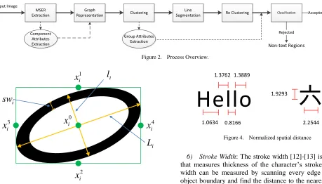
An overview diagram of our framework is illustrated in Fig.2. Our method is a MSER based scheme that is modified from [11] by applying the double-threshold scheme with cascade chain decision and modifying the features in order to make the framework more robust to the language variation and text alignments. The MSER algorithm can provide the interest regions for text candidates. Attributes such as area, position, color, size, and stroke width are extracted for each MSER component. Linkage clustering is applied to group the MSERs with have the similar properties. By using graph representation, every MSER component is modeled as a node in the graph. The connectivity between each pair of MSER components is defined based on differences of the component’s attributes. After the clustering process, a line segmentation process is applied to break the groups that contain outliers or multiple text lines. The final process is the text and non-text classification. We develop the double- threshold scheme with the cascade constraint decision chain for recognizing text cluster. The system initially categorizes the groups of MSERs into three classes that are text regions with high confidence (THC), text regions with low confidence (TLC) and non-text regions (NT). The different threshold levels are used to determine the text regions with high and low confidences. The final text regions are collected from all THCs and TLCs that are connected to at least one THCs. Details of each process are described in the following sections.

A. MSER Extraction

The MSER [16] is a method to detect contours of the homogeneous connected regions in the image. In gray-scale images, the MSERs can be extracted by intensity thresholding. By increasing the threshold level, contours of the areas that have intensity over the current threshold are compared with the results in the previous threshold level. The MSER is acquired when the considered contour is stable in two consecutive thresholds.

The MSER algorithm is used as an initial process for extracting the interest regions that might be parts of texts. It can detect homogenous regions that have intensities contrasting to their boundary pixels. The MSER method can be used to extract the text areas, because texts tend to have distinct colors contrasting to their background. In this work, we set an upper bound of the number of MSER components that will be extracted from the image. Some MSER components are removed in this step based on size and aspect ratio criteria. The result of this step is denoted as a set of MSER components

}

,...,

,

{

C

1

C

2

C

M



C

where

C

_i represents a list of pixels

that belong to the

i

-th MSER component.

B. Attributes of MSER Components

After the MSER extraction process, the following attributes are determined for every MSER component

C

_i.

Figure 1. Examples of different character structures and text line structures from various languages.

English Japanese

1) Area : The area is defined as the number of pixels in the MSER component. The area of the component

C

_i is denoted as

A

_i.

2) Spatial Position: There are five points that are collected as the spatial position attribute of each component

C

_i. The first point used here is a centroid of the component denoted by

) 0 (

i

x

where

x

represents a pixel coordinate

(

x

,

y

)

. The other four points which are denoted by

x

(_i1),

x

(_i2),

x

(_i3), and

x

_i(4) are the middle points of top, bottom, left, and right bounding box’s edges, respectively. Fig. 3 shows an illustration for the definition of five points of the spatial position attribute.

3) RGB Color: The RGB color attribute is defined as median of red (

r

), green (

g

) and blue (

b

) color components of pixels that belong to the corresponding MSER component.

i

c

represents a vector of RGB color elements

(

r

,

g

,

b

)

of the component

C

_i.

4) Length of Major Axis: Length of the major axis

L

_i is an attribute that indicates the maximum distance between two pixels in the component

C

_i.

5) Length of Minor Axis: Along with the major axis, length of the minor axis

l

_i is determined as the maximum distance between two pixels along the direction that is perpendicular to the major axis in the component

C

_i. Fig. 3 shows the illustration for the definition of length of major and minor axes.

6) Stroke Width: The stroke width [12]-[13] is a parameter that measures thickness of the character’s stroke. The stroke width can be measured by scanning every edge pixel in the object boundary and find the distance to the nearest edge pixel along the gradient direction of that pixel [12]. In this work, we use an average of stroke width calculated from each edge pixel as one of the attributes for measuring of the size of MSER component. Fig. 3 shows the illustration for the definition of stroke width.

sw

_i denotes the average stroke width for the component

C

_i.

7) Stroke Width Variance: Along with the average stroke width, variance of the stroke width value of the edge pixels is also calculated. Since the text components are typically the bands of approximately constant width, the stroke width variance extracted from the text components should be small.

i

swv

denotes the stroke widthvariance of the component

C

_i.

C. Graph Representation

In clustering process, we model the MSER components and their connectivity as an undirected graph.

C

_i represents a node of the graph which is corresponding to each MSER components.

w

_ij represents a weight of the edge connecting between node

C

_i and

C

_j. The weights are determined based on spatial distance, color difference, size difference and stroke width difference between each node. The definition of each parameter is given as following.

1) Normalized Spatial Distance: The spatial distance ij

SPD

is a parameter that measures the geomatric distance

between two components. In this work,

SPD

_ij is defined as







)

,

min(

min

( ) ( )

,

j i

q j p i q p ij

l

l

SPD

x

x





 (1)

Figure 2. Process Overview.

Figure 3. Attributes of MSER components.

Figure 4. Normalized spatial distance

MSER Extraction Input Image

Component Attributes Extraction

Graph

Representation Clustering

Group Attributes Extraction

Line

Segmentation Text Regions

Non-text Regions

Re Clustering Classification Accepted

Rejected

2

i

x

3

i

x

x

_i4

1

i

x

l

i

i

L

0

i

x

i

sw

Hello

1.3762

1.0634 0.8166 1.3889

六

1.9293 2.0276

ij

SPD

is the minimum euclidian distance between any pair of

key position

x

_i(p) and

x

(_jq) of the component

C

_i and

C

_j that is normalized by the minimum minor axis of these two components. The normalization process is applied to obtain a scale-invariant property. Examples of values of

SPD

computed from Chinese and English texts are given in Fig. 4.

2) Color Difference: The color difference

CLD

_ij is a parameter that measures the difference of the RGB color between two components.

CLD

_ij can be calculated by

 . (2)

3) Size Difference: The size difference

SZD

_ij is a parameter that measures a ratio of the bounding box’s size of two components.

SZD

_ij is defined as

. (3)

4) Stroke Width Difference: The stroke width difference ij

SWD

is a parameter that measures a ratio of the average

stroke width of two components.

SWD

_ij is defined as



















j i ij

sw

sw

SWD

log

. (4)

In order to determine the weight

w

_ij connecting to the node

C

_i, the system determines a set of neighbor node candidates as



























SW ij SZ ij CL ij SP ij j i

T

SWD

T

SZD

T

CLD

T

SPD

C

,

,

N

. (5)

where

N

_i denotes the set of neighbor node candidates of

C

_i

.

SP

T

,

T

_CL,

T

_SZ and

T

_SW are cut-off thresholds for the spatial distance, color difference, size difference and stroke width difference, respectively. According to (5), the neighbor candidates are defined as nearby components with similar color, size and stroke width.

j i ij

CLD



c



c























j j i i ij

l

L

l

L

SZD

log

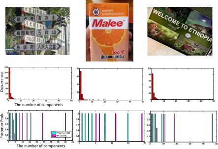
Figure 5. Histograms of the number of components and posterior probabilities

0 10 20 30 40 50

0 20 40 60 80

0 10 20 30 40 50

0 20 40 60 80 100 120

0 10 20 30 40 50

0 20 40 60 80 100

0 5 10 15 20 25 30 35 40 45

0 0.2 0.4 0.6 0.8 1

P(NonText | NC) P(Text | NC)

0 5 10 15 20

0 0.2 0.4 0.6 0.8 1

The number of components

Occurr

ence

The number of components

Pos

terior

Pr

ob.

0 10 20 30 40 50

To limit the number of connection in each node, the

K

nearest node of

C

_i is searched within the set of neighbor candidates

N

_i. Finally, the weight

w

_ij is defined as















otherwise

;

0

)

(

or

)

(

and

;

1

_{j i i j}

ij

C

KNN

C

C

KNN

C

j

i

w

, (6)

where

KNN

(

C

i

)

represents a set of

K

nearest neighbor nodes of node

C

_i obtained by searching in the set of neighbor node candidates

N

_i and using only

SPD

as a distance measure.

w

ij



1

means there is a link between components

i

C

and

C

_j while

w

_ij



0

means there is no link between components

C

_i and

C

_j.

We use the parameter

K

for controlling the number of maximum connection in each node. In English language, only two connections allowed for each node should be enough for connecting the left and right text neighboring components in line structure of the English sentence. On the other hand, in Chinese language, to cover the connection of every connected component in intra-character and neighboring characters, three to five connections are required.

D. Clustering

In this stage, the connected components are group together.

}

,...,

,

{

G

1

G

2

G

M



G

denotes a set of group of connected

components where each group

G

_p is a set of components

C

_i

which satisfy the following three constraints.

1) In each group

G

_p



G

, for every

C

_i



G

_p, there is at least one component

C

_j



G

_p that

w

_ij



1

.



,





1









p

i

j

C

_i

C

_j

G

_p

w

_ij (7)

2) In every pair of group

G

_p

,

G

_q



G

and

p



q

, there is no component

C

_i



G

_p and

C

_j



G

_q that

w

_ij



1

.





p



q



i



j



p



q

,

C

_i



G

_p

,

C

_j



G

_q

w

_ij



0



  3) Every component

C

_i belongs to only one group.















p

q

G

_p

G

_q , and (9)

C











G

G

G

N

G

1 2 3



(10)

E. Line Segmentation

The clusters or groups that we obtain from the clustering process may contain characters from multiple lines in sentence structure or sometimes the non-text components are mixed with the text components. In order to improve the clustering results, the line segmentation process is applied by removing the connecting edges with the outlier orientation.

The process starts from identifying the major direction

p



of all connecting edges in each group by separating the edge directions into several bins and finding the bin that have maximum votes. The edge direction



_ij represents the geometric orientation of the vector from component

C

_i to

j

C

. As a result,



_ij is defined as the orientation of the vector from position

x

(_i0) to

x

(_j0).

The system removes the connecting edges between component

C

_i and

C

_j by setting

w

ij



0

, if



ij





p is

over the threshold. After every outlier directions are eliminated and the connectivity of the graph is updated, the clustering process is repeated again to refine the set of connected components.

F. Group Attributes

After MSER components have been grouped together, the following attributes are determined for every group of component

G

_i.

Figure 6. Example of polynomial regression using different reference points.

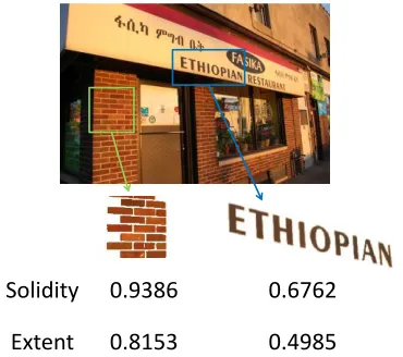
Figure 7. Exmples of extent and solidity in groups of MSER component.

tool

Solidity

Extent

0.9386

0.6762

1) The Number of Components: The number of members in each group is counted. Based on the observation, the groups with few members tend to be non-text regions; therefore, the number of components can be used as one attribute to filter out the non-text groups. The number of components in

G

_i is denoted by

NC

_i

.

Some examples of histogram distribution of

NC

are illustrated in Fig. 5. The images in the middle row shows the histogram of

NC

analyzed from the images in the top row. The distribution is mainly located in one or two connected component(s). The images in the last row shows comparison of the posterior probabilities of

P

(

Text

NC

)

and

P

(

Nontext

NC

)

.

The posterior probability distributions show that

P

(

Nontext

NC

)

is much more higher than

P

(

Text

NC

)

when

NC

is small.

2) Residual Errors of Polynomial Regression: The residual error of the polynomial regression is a parameter to measures a geometrical structure of the component alignment. In general, texts are clustered in the line structures; therefore, the residual errors of the polynomial regression tend to be small for the text clusters. The residual error will become zero when the cluster aligns as a straight line. Since the best referrence points of alignment for curve fitting may be different as shown in Fig. 6, in this work, we use five points of the spatial position attribute as the referrence points for polynomial curve fitting. As a result, the residual error of the polynomial regression can be defined as





 



i j G

C j i

k i k i

L

NC

PRE

1

)

(

min

( )

] 4 , 0

[



_

(11)

where

PRE

_i is the residual error attribute of group

G

_i and )

(k i



is defined as a residual errors of polynomial curve fitting

of set of spatial positions



x

(_jk)

C

_j



G

_i



. According to (11), to obtain the scale invarient property, the residual errors is normalized by an average length of the major axes of the components in that group.

3) Stroke Width Variance: The average stroke width varience

SWV

_i is defined as









i j G

C

j i

i

swv

NC

SWV

1

 (12)

SWV

tends to be a small value for the text regions and high for the non-text regions.

4) Average Extent: The extent is defined as a ratio of the area of the component to the area of the component’s bounding box. The average extent

EXT

_i of each component

i

G

is computed as an attribute of the group.

5) Average Solidity: Similar to the extent, the solidity is defined as a ratio of the area of the component to its corresponding convex area. We can use the solidity and extent to classify some groups of solid pixel distribution like brick walls as shown in Fig. 7. The solidity attributes of each group is defined as an average solidity of every component in that group.

SLD

_i denotes the average solidity in the group

G

_i

.

6) The Number of Holes: The number of holes is one of the parameters that can identify the non-character components. Typically, there is a few holes in the text’s characters. In the proposed scheme, the number of holes appearing in each group

G

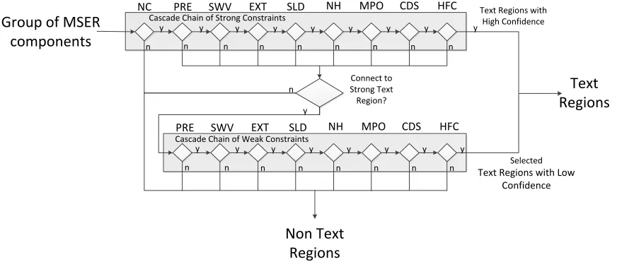
_i is counted and normalized with the number of connected components in that group to obtain the average

Figure 8. The propsoed double-thresold scheme for text and non-text classification

Group of MSER

components

NC

Text

Regions

Non Text

Regions

Cascade Chain of Strong Constraints

Cascade Chain of Weak Constraints

PRE SWV EXT SLD NH MPO CDS HFC

PRE SWV EXT SLD NH MPO CDS HFC

Connect to Strong Text Region?

Text Regions with High Confidence

Selected

Text Regions with Low Confidence

y n

n n n n n n n n

n n n n n n n n

y y y y y y y y

n

y

number of holes in one connected component.

NH

_i

represents the average number of holes per connected component in group

G

_i.

7) Maximum Probability in Histogram of Connecting Edge Orientation: To identify the uniqueness of the directions of connecting edges in the group. The normalized histogram of edge orientation is extracted for each group. The maximum probability

MPO

_i is defined as the maximum value of the histogram of group

G

_i which represents the uniqueness of the connecting edge directions.

8) Centroid Distance Signature Score: This attribute is extracted by collecting the distance from the component’s centriod to each pixels in the component’s boundary called centroid distance signature. Then, the centroid distance signature are filtered by using a high-pass filter. An average power of the filtered centroid distance signature of every components are used as the centriod distance signature score

i

CDS

. This attribute is used for measuring the roughness of the component’s boundary. For example, some characters that have smooth boundary will get low energy, while the components with very rough boundary such as leafs will get high energy.

9) Haralick’s Feature Classification Score: In this work, we also apply the textural based features to classify the component. A gray level cooccurance matrix (GLCM) [15] is extracted from the image by varying the directions, offset values and color channel in YCbCr space. Three Haralick’s features (contrast, energy and homogeneity) are extracted from each GLCM. A neural network is trained to classify the text and non-text components based on these textural features. The Haralick’s feature classification score

HFC

i is an average

output from the neural network (classification confidence) obtained from every component in

G

_i.

G. Group Classification

The final step in our text localization process is to classify the group. In this work, we proposed the double-threshold scheme in the cascade decision structure as shown in Fig. 8. Similar to Canny edge detection, we initially divide the groups of components into three classes that are THC, TLC and NT. According to Fig. 8, we have double levels of threshold or constraints called strong constraints and weak constraints. The THCs are the regions that satisfy all strong constraints of the group attributes. The constraint for each attributes can be determined from the posterior or likelihood probability collected from the training samples. The sequence of constraint checking is designed to minimize the computational cost. For example, the first constraint is

NC

that is very easy to find and can filter out a large number of components as shown in Fig. 5. Only a few components are left for the Haralick’s feature extraction which requires the highest cost. All of THC’s components will finally be classified as the text regions. On the other hand, TLCs are defined as groups of components that satisfy all weak constraints but fail to satisfy some strong constraints. Only TLCs that connect to any THCs will finally be classified as the text regions while the other TLCs are rejected. The connectivity between TLCs and THCs are determined by normalized spatial distance, mean of major axis difference, group color difference and group stroke width difference.

IV. EXPERIMENTAL RESULTS

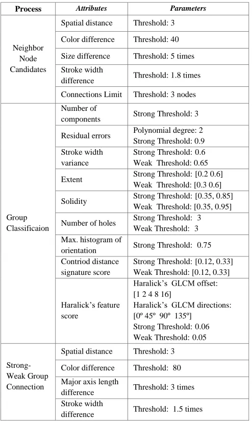
In this experiment, fifty natural scene images composed of many languages such as English, Chinese, Japanese, Korean, Arabic, and Thai with various text alignments and camera views are collected and used for testing the performance of the proposed scheme. In this experiment, the parameters and thresholds used in our proposed methods was set as shown in Table I. We evaluate the result of our process compare to H. Chen’s method [10]. The result is evaluated by measuring precision and recall based on a text line oriented evaluation. If the text regions obtained from the systems contain more than 80% of all characters in the actual text lines, they are considered

TABLE I. PARAMETERS AND THRESHOLDS USED IN THE EXPERIMENT

Process Attributes Parameters

Neighbor Node Candidates

Spatial distance Threshold: 3

Color difference Threshold: 40

Size difference Threshold: 5 times

Stroke width

difference Threshold: 1.8 times

Connections Limit Threshold: 3 nodes

Group Classificaion

Number of

components Strong Threshold: 3

Residual errors Polynomial degree: 2

Strong Threshold: 0.9 Stroke width

variance

Strong Threshold:0.6 Weak Threshold: 0.65

Extent Strong Threshold:[0.2 0.6]

Weak Threshold: [0.3 0.6]

Solidity Strong Threshold:[0.35, 0.85]

Weak Threshold: [0.35, 0.95]

Number of holes Strong Threshold: 3

Weak Threshold: 3 Max. histogram of

orientation Strong Threshold: 0.75

Contriod distance signature score

Strong Threshold:[0.12, 0.33] Weak Threshold: [0.12, 0.33]

Haralick’s feature score

Haralick’s GLCM offset: [1 2 4 8 16]

Haralick’s GLCM directions: [0º 45º 90º 135º]

Strong Threshold:0.06 Weak Threshold:0.05

Strong-Weak Group Connection

Spatial distance Threshold: 3

Color difference Threshold: 80

Major axis length

difference Threshold: 3 times

Stroke width

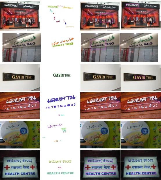
Figure 9. Example of experimental results. From left to right, original scene images, text localization result from the proposed method (different colors are corresponding to different text cluster), the result (bounding box) from H. Chen method [10] using dark texts in brighter background ,the result from H. Chen method using bright texts in

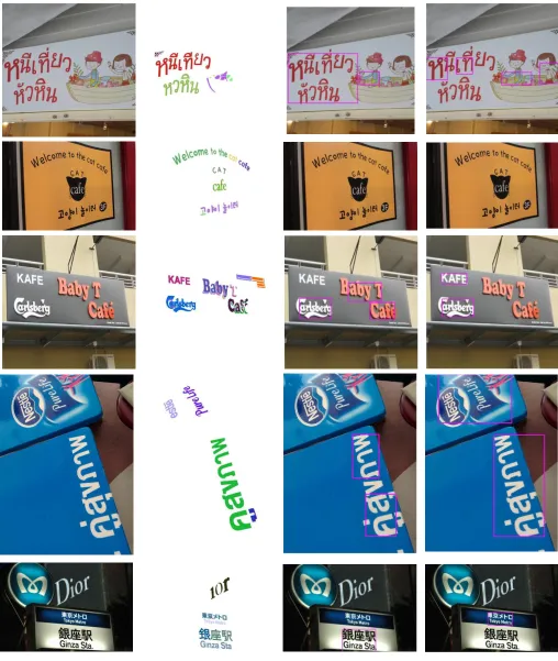
Figure 10. Example of experimental results (continued). From left to right, original scene images, text localization result from the proposed method (different colors are corresponding to different text cluster), the result (bounding box) from H. Chen method [10] using dark texts in brighter background ,the result from H. Chen method using

as true positives. On the other hand, the detected text regions which do not contain the text lines are considered as false positives. The text lines that cannot be found by the systems are considered as false negatives. The reason why we did not use a word oriented evaluation which is widely used for evaluation of the English text localization is that many languages in the test set have no space between the words as in English and the word segmentation problem is still not included in this work.

Some example images of the results are demonstrated in Fig. 9-10. The first column illustrates the original images. The second column shows the text regions obtained from our proposed method. The last two columns are the result from [10] that has two assumptions. The first assumption is that the texts are appearing in the brighter background, while the second assumption is that there are brighter texts appearing in darker background. Based on the results of this multi-language dataset with large variation in text alignments and camera views, we obtain the precision of 70.16% and the recall of 93.06% while H. Chen’s method obtains the precision of 44.76% and the recall of 44.44%.

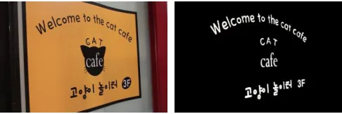
In this experiment, the proposed method is also evaluated based on a pixel-wise evaluation to observe the precision and recall in term of the areas that systems can be detected. Ground truth images are prepared as binary masks of text regions as shown in Fig. 11. By comparing the binary masks of text regions obtained from the proposed method to the ground truth, we can obtain the precision of 59.38% and recall of 74.91%.

V. CONCLUSIONS

The MSER based text localization using double-threshold scheme was presented in this paper. The objective of this work is to develop the framework to detect the texts in natural scene images that is robust to languages, text alignments, text line structures, and camera views. The MSER algorithm is used to initialize the regions of text candidates. The MSERs with similar properties are grouped. The groups are classified by using the double-threshold scheme. In the classification process, the short-circuit evaluation is used to reduce the complexity of the attributes extraction process. The groups that satisfy the set of strong constraints are labeled as text. The groups that do not satisfy the set of weak constraints are rejected. The groups that satisfy the set of weak constraints but do not satisfy any strong constraints are labeled as text if they are connecting to the groups that satisfy the strong constraints. Based on the experiment on the multi-language dataset, our proposed scheme yields the precision of 70.16% and recall of 93.06% based on the text line oriented evaluation.

ACKKNOWLEDGEMENTS

This research was supported by Graduate School, Chiang Mai University, Thailand.

REFERENCES

[1] C. Yi, Y. Tian, and A. Arditi, “Portable Camera-Based Assistive Text and Product Label Reading From Hand-Held Objects for Blind Persons”, IEEE/ASME Transactions on Mechatronics, Vol. 19, No. 3, pp. 808 – 817, 2014.

[2] R. Pimup, A. Kawewong, and O. Hasegawa, “Fast Online Incremental Aapproach of Unseen Place Classification Using Disjoint-Text Attribute Prediction” 19th IEEE International Conference on Image Processing (ICIP), pp 3141 – 3144, 2012.

[3] X. Liu, and J. Samarabandu, “An Edge-based Text Region Extraction Algorithm for Indoor Mobile Robot Navigation”, International Conference on Mechatronics & Automation, Vol. 2, pp. 701-706, 2005. [4] H. Yang and C. Meinel, “Content Based Lecture Video Retrieval Using

Speech and Video Text Information”, IEEE Transactions on Learning Technologies, Vol. 7, No. 2, pp. 142-154, 2014.

[5] K. Jung, K. I. Kim and A. K. Jain, “Text information extraction in images and video: a survey”, Pattern Recognition, Vol. 37, No. 5, pp. 977-997, May 2004

[6] S. M. Hanif and L. Prevost, “Text Detection and Localization in Complex Scene Images using Constrained AdaBoost Algorithm”, 10th

International Conference on Document Analysis and Recognition, pp. 1-5, 2009.

[7] L. Neumann and J. Matas, “Real-Time Scene Text Localization and Recognition”, 25th _{IEEE Conference on Computer Vision and Pattern}

Recognition, pp. 3538-3545, 2012.

[8] A. V.Pillai, A. A. Balakrishnan, R. A. Simon, R. C Johnson and S. Padmagireesan, “Detection and Localization of Texts from Natural Scene Images using Scale Space and Morphological Operations”, 2013

International Conference on Circuit, Power and Computing

Technologies, pp. 880-885, 2013.

[9] B. Epshtein, E. Ofek, and Y. Wexler, "Detecting text in natural scenes with stroke width transform", IEEE Conference on Computer Vision and Pattern Recognition, pp.2963-2970, June 2010.

[10] H. Chen, S.S. Tsai, G. Schroth, D.M. Chen, R. Grzeszczuk and B. Girod, "Robust text detection in natural images with edge-enhanced Maximally Stable Extremal Regions," 18th _{IEEE International Conference on Image}

Processing, pp.2609-2612, Sept. 2011.

[11] X. Yin, X. Yin, K. Huang and H. Hao, “Robust Test Detection in Natural Scene Images”, IEEE Transactions on Pattern Analysis and Machine Intelligence, Vol. 36, No. 5, pp. 970-983, May 2014.

[12] B. Epshtein, E. Ofek and Y. Wexler, “Detecting text in natural scenes with stroke width transform”, IEEE Conference on Computer Vision and Pattern Recognition 2010, pp. 2963-2970, June 2010.

[13] K. Subramanian, P. Natarajan, M. Decerbo and D. Castanon, "Character-Stroke Detection for Text-Localization and Extraction", 9th _{International}

Conference on Document Analysis and Recognition , vol.1, pp.33-37, Sept. 2007.

[14] K. Jung, K. Kim, T. Kurata, M. Kourogi, J. Han, “Text scanner with text detection technology on image sequence”, International Conference on Pattern Recognition, Vol. 3, Quebec , pp. 473–476. Canada, 2002 [15] J. Zhang and Y. Chong, “Text Localization based on the Discrete

Shearlet Transform”, 4th

IEEE International Conference on Software Engineering and Service Science, pp.262-266, May 2013.

[16] J. Matas, O. Chum, M. Urban, and T. Pajdla, "Robust wide baseline stereo from maximally stable extremal regions", British Machine Vision Conference, pp. 384-396, 2002

[17] Robert M Haralick, K Shanmugam, Its'hak Dinstein (1973). "Textural Features for Image Classification". IEEE Transactions on Systems, Man, and Cybernetics. SMC-3 (6): 610–621.