Numerical solution of nonlinear third order Van der Pol oscillator

(1)

~ 24 ~ WWJMRD 2019; 5(12): 24-28

www.wwjmrd.com International Journal Peer Reviewed Journal Refereed Journal Indexed Journal

Impact Factor MJIF: 4.25 E-ISSN: 2454-6615

Gilder Cieza Altamirano

Department of General Studies, National Autonomous University of Chota, Peru

Rafaél Artidoro Sandoval Núñez

Correspondence:

Gilder Cieza Altamirano

Numerical solution of nonlinear third order Van der

Pol oscillator

Gilder Cieza Altamirano, Rafaél Artidoro Sandoval Núñez

Abstract

In the present study, numerical investigations have been carried out for solving a class of third order Van der Pol oscillator for differential equation related to nonlinearity for both parameters based on stiff and non-stiff conditions. The variants of the proposed scheme have been numerically solved and the comparison of results are presented based on the two schemes named as Adams numerical scheme and implicit Runge-Kutta scheme which is used to solve the third order nonlinear Van der Pol oscillator. The details of the achieved numerical results in the form of tables have been numerically discussed.

Keywords: Third order Van der Pol oscillator, Adams method, implicit Runge-Kutta method, nonlinear, stiff, non-stiff

1. Introduction

The angular frequency based functions having the derivatives of first order has achieved diverse attention of the researchers community using the models of nonlinear oscillators [1-4]. Recently, these schemes represent generally the nonlinear differential equations of second-order. A superior class of an oscillatory system is called oscillator of Van der Pol that is used to govern nonlinear damping and represent the second-order nonlinear ordinary differential model. In this study we solve the nonlinear third order Van der Pol oscillator which is basically a third order differential equation. The generic form of nonlinear third order Van der Pol equation is given as:

2

2 3

1 2

3 2

3

d

d u

du

(

1)

(

1)

0, 0

d

u

d

u

d

u

x

X

x







x







x

 

 

(1) 2

2

(0)

2,

du

0,

d u

0. u

dx



The above model is presented on the basis of second order Vander-pol oscillators which is extensively used in science, engineering and has the huge amplitude planner flexural free sensations of an inextensible slender cantilever beam component [5]. Jockon and Mickens [6] accessible the comprehensive fundamental study for the second order nonlinear oscillators and familiarized the generic properties of the oscillator. Additionally, Van der pol oscillator rises in many submissions of engineering and applied science. Numerous methods have been applied to solve these types of models. By keeping a view on it, a good variety and source of assessment article [7] has been obtainable in which variety of numerical techniques for nonlinear Van der Pol oscillators are nominated in detail.

The goal of the present investigation is to explore and exploit a class of nonlinear third order Van der Pol oscillators using Adams method and Implicit Runge-Kutta method. In this regard, two numerical problems based on third order nonlinear Van der Pol oscillators along with two cases of each have been present and results are checked from two schemes that are found to be accurate.

(2)

The remaining parts of the article is organized as follows: Section 2 narrates the numerical technique, the numerical outcomes are provided in Section 3 and conclusions along with future research directions are listed in the final Section.

2. Numerical methods

In this study section, the communications based on deterministic and stochastic numerical solvers have been effected generally in extensive fields, for example linear/ nonlinear algebraic models [8], nanotechnology based equations [9], system of nonlinear doubly singular equations [10], model based on Thomas-Fermi equations [11], an extensive class of delay differential second order

equation [12] and boundary value problems based on multi-point equations [13]. In this study, predictor-corrector numerical Adams scheme and numerical Implicit Runge-Kutta method are applied to solve the third order nonlinear Van der Pol oscillators.

2.1. Predictor-corrector Adams numerical technique

To find the numerical solution of nonlinear third order Van der Pol oscillator, the corrector- predictor numerical scheme is applied that takes two stages to complete further. The approximate outcomes of prediction is accomplished in the first step, while to find the numerical outcomes of correction is proficient with the same contributions of prediction.

   

,

0 0

du

h x u

u

x

u

dx



. (2)

Two steps for the generalized Adams-Bashforth numerical technique by using the predictor-corrector scheme:









1 1 1

3

1 ,

,

2

n n n n n n

D

_



u



fh

x

u



fh

x

_

u

_

. (3)

Adams-Moulton two-stage corrector is provided as:



 







1 1 1

1 ,

,

.

2

n n n n n n

u

_



u



f h

x

_

D

_



h

x

u

₍₄₎

The 4-steps predictor corrector is as follows:





















1

55 ,

59

1

,

1

37

2

,

2

9

3

,

3

.

24

n n n n n n n n n n

D

_



u



f

h

x

u



f

x

_

u

_



f

x

_

u

_



f

x

_

u

_ ₍₅₎

The 4-step Adams-Bashforth Moulton is given as:





















1

9

1

,

1

19 ,

5

1

,

1 2

,

2

.

24

n

u

n

h

n

D

n

f

n

u

n

f

n

u

n n n

f

u







x

 



x



x

 



f

x



u

 (6)

2.2. Implicit Runge-Kutta numerical technique

To solve the nonlinear Van der Pol oscillator, the Implicit

Runge-Kutta technique is designed. The generic form of Implicit Runge- Kutta technique is considered as:





1 1

1

,

s

n n j j n n

j

u

f

b k k

h

x

u

_









(7)









2 n 2

,

n 21 1

k



h

x



c

f

u



f a k

,









3 n 3

,

n 31 1 32 2

,

k



h

x



c

f

u



f a k



a

k

….







,

1 1 2 2

...

1 1



s n s n s s ss s

k



h

x



c

f

u



f a k



a k

 

a

_

k

_

.

In the first step, to consider the obtained initial outcomes and slopes are documented for all variables. Taking these

achieved numerical outcomes for slopes (the

k

1s_{) at the}

central point of the interval to form the designs of the dependent variable. In the second step, the slopes of the

middle-point (the

k

2s_{) are achieved by taking these}

attained mid-point values. The designed numerical

originate to the new slope of predictions at middle-point

(the

k

3s_{). These numerical values are supplementary}

applied to create predictions to development slopes at the

final point of the interval (the

k

ss_{). Likewise, all the}

outcomes for

k

s_{are achieved composed to make another}

(3)

~ 26 ~

3. Results and Discussions

In this section, numerical experimentations are presented for nonlinear third order Van der Pol Oscillators with stiff

and non-stiff parameters. Two problem along with two cases have been solved and their numerical results are tabulated in Tables 1 and 2.

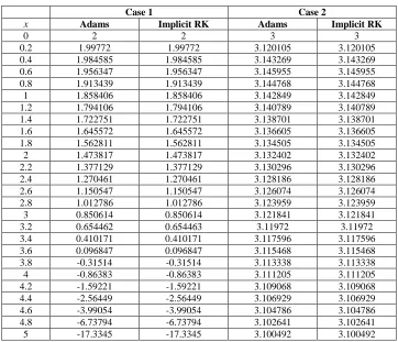
Problem 1

Case 1: Consider the Van der Pol Oscillator with non-stiff conditions for



1



1

_and



2



1

2

3 2

3 2 3

d

d u

du

(

1)

(

1)

0, 0

d

x

u

d

u

d

x

u

x

X

u

x









 

 

(8) 2

2

(0)

2,

du

0,

d u

0. u

dx



Case 2: Consider the Van der Pol Oscillator with non-stiff conditions for



1



5

_and



2



10

2

3

2 3

d

d u

du

5(

1)

10(

1)

0, 0

d

x

u

d

x

u

d

x

u

x

X

u









 

 

(9) 2

2

(0)

3,

du

1,

d u

0. u

dx



To find the numerical result of the problems, we have applied the Adams and Implicit Runge-Kutta by using the Mathematica built in functions presented in Table 1 and Table 2. The results calculated for the both methods of the two problems are given in Table 1 and Table 2 for inputs

 

0,1

t

ò

_{with a step size of}

_0.1

_{. It is cleared that the}

proposed solutions show same results as of Adams and Implicit Runge-Kutta results and proved very good agreements.

Table 1: Comparison of Adams and Implicit Runge-Kutta for case 1 and case 2

Case 1 Case 2

x Adams Implicit RK Adams Implicit RK

0 2 2 3 3

0.2 1.99772 1.99772 3.120105 3.120105

0.4 1.984585 1.984585 3.143269 3.143269

0.6 1.956347 1.956347 3.145955 3.145955

0.8 1.913439 1.913439 3.144768 3.144768

1 1.858406 1.858406 3.142849 3.142849

1.2 1.794106 1.794106 3.140789 3.140789

1.4 1.722751 1.722751 3.138701 3.138701

1.6 1.645572 1.645572 3.136605 3.136605

1.8 1.562811 1.562811 3.134505 3.134505

2 1.473817 1.473817 3.132402 3.132402

2.2 1.377129 1.377129 3.130296 3.130296

2.4 1.270461 1.270461 3.128186 3.128186

2.6 1.150547 1.150547 3.126074 3.126074

2.8 1.012786 1.012786 3.123959 3.123959

3 0.850614 0.850614 3.121841 3.121841

3.2 0.654462 0.654463 3.11972 3.11972

3.4 0.410171 0.410171 3.117596 3.117596

3.6 0.096847 0.096847 3.115468 3.115468

3.8 -0.31514 -0.31514 3.113338 3.113338

4 -0.86383 -0.86383 3.111205 3.111205

4.2 -1.59221 -1.59221 3.109068 3.109068

4.4 -2.56449 -2.56449 3.106929 3.106929

4.6 -3.99054 -3.99054 3.104786 3.104786

4.8 -6.73794 -6.73794 3.102641 3.102641

5 -17.3345 -17.3345 3.100492 3.100492

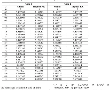
Problem 2

(4)

3

2

2 3

2

d

d u

du

500(

1)

(

1)

0, 0

d

u

d

u

d

x

u

x

X

u

x





x





 

 

2

(0)

5,

du

1,

d u

0. u

dx



(10)

Case2: Consider the Van der Pol Oscillator with stiff conditions for



1



1000

_and



2



1

2

2 3

3 2 3

d

d u

du

1000(

1)

(

1)

0, 0

d

u

d

u

d

x

u

x

X

u

x





x





 

 

(11) 2

2

(0)

3,

du

1,

d u

0. u

dx



Table 2: Comparison of Adams and Implicit Runge-Kutta for case 1 and case 2

Case 1 Case 2

x Adams Implicit RK Adams Implicit RK

0 5 5 3 3

0.2 5.199783 5.199783 3.199927 3.199927

0.4 5.399122 5.399122 3.399702 3.399702

0.6 5.598003 5.598003 3.599319 3.599319

0.8 5.796412 5.796412 3.798773 3.798773

1 5.994337 5.994337 3.998055 3.998055

1.2 6.191762 6.191762 4.197159 4.197159

1.4 6.388675 6.388675 4.396078 4.396078

1.6 6.585061 6.585061 4.594806 4.594806

1.8 6.780908 6.780908 4.793334 4.793334

2 6.976203 6.976203 4.991657 4.991657

2.2 7.170932 7.170932 5.189767 5.189767

2.4 7.365083 7.365083 5.387658 5.387658

2.6 7.558642 7.558642 5.585321 5.585321

2.8 7.751597 7.751597 5.78275 5.78275

3 7.943935 7.943935 5.979938 5.979938

3.2 8.135644 8.135644 6.176878 6.176878

3.4 8.326712 8.326712 6.373562 6.373562

3.6 8.517127 8.517127 6.569984 6.569984

3.8 8.706877 8.706877 6.766137 6.766137

4 8.89595 8.89595 6.962014 6.962014

4.2 9.084335 9.084335 7.157607 7.157607

4.4 9.27202 9.27202 7.35291 7.35291

4.6 9.458994 9.458994 7.547915 7.547915

4.8 9.645247 9.645247 7.742617 7.742617

5 9.830767 9.830767 7.937008 7.937008

4. Conclusion

In the present study, the numerical treatment based on third order nonlinear stiff/ non-stiff Van der Pol oscillator presented by manipulating the strength of the numerical Adams scheme and Implicit Runge-Kutta scheme. The numerical results are found to be accurate and consistent from both of the schemes. The proposed scheme is valuable and appropriate for solving linear/nonlinear second order Van der Pol oscillator for two problems each has two cases. The software used for solving the nonlinear second order Van der Pol oscillator is Mathematica 10.4.

In future, this scheme is applied to solve nonlinear system of second order and third order Van der Pol oscillators.

References

1. Kovacic, I., 2011. Forced vibrations of oscillators with a purely nonlinear power-form restoring force. Journal of Sound and Vibration, 330(17), pp.4313-4327. 2. Mickens, R.E. and Oyedeji, K., 2011. Comments on

(1+ x˙ 2) x= 0. Journal of Sound and Vibration, 330(17), pp.4196-4200

3. Feng, J., Zhu, W.Q. and Liu, Z.H., 2011. Stochastic optimal time-delay control of quasi-integrable Hamiltonian systems. Communications in Nonlinear Science and Numerical Simulation, 16(8), pp.2978-2984.

4. Eigoli, A.K. and Khodabakhsh, M., 2011. A homotopy analysis method for limit cycle of the van der Pol oscillator with delayed amplitude limiting. Applied

Mathematics and Computation, 217(22), pp.9404-9411.

5. Hamdan, M.N. and Shabaneh, N.H., 1997. On the large amplitude free vibrations of a restrained uniform beam carrying an intermediate lumped mass. Journal of Sound and Vibration, 199(5), pp.711-736.

(5)

~ 28 ~ 7. Kerschen, G., Worden, K., Vakakis, A.F. and Golinval,

J.C., 2006. Past, present and future of nonlinear system identification in structural dynamics. Mechanical systems and signal processing, 20(3), pp.505-592. 8. Raja, M. A. Z., Sabir, Z., Mehmood, N., Al-Aidarous,

E. S., & Khan, J. A. (2015). Design of stochastic solvers based on genetic algorithms for solving nonlinear equations. Neural Computing and Applications, 26(1), 1-23.

9. Mehmood, A., Zameer, A., & Raja, M. A. Z. (2018). Intelligent computing to analyze the dynamics of Magnetohydrodynamic flow over stretchable rotating disk model. Applied Soft Computing, 67, 8-28.

10. Raja, M. A. Z., Mehmood, J., Sabir, Z., Nasab, A. K., & Manzar, M. A. (2017). Numerical solution of doubly singular nonlinear systems using neural networks-based integrated intelligent computing. Neural Computing and Applications, 1-20.

11. Sabir, Z., Manzar, M. A., Raja, M. A. Z., Sheraz, M., & Wazwaz, A. M. (2018). Neuro-heuristics for nonlinear singular Thomas-Fermi systems. Applied Soft Computing, 65, 152-169.

12. Sabir, Z., Umar, M. and Unlu, C., Solving a Class of Second Order Delay Differential Equation by Using Adams and Implicit Runge-Kutta Method.