Fast and Robust Method for Dynamic Gesture Recognition Using Hermite Neural Network

Fast and Robust Method for Dynamic Gesture

Recognition Using Hermite Neural Network

Wensheng Li, Chunjian Deng

Zhongshan Institute, University of Electronic Science and Technology of China, Zhongshan,China Email: [email protected]

Abstract—Due to its shortcomings such as slow convergence rate and low recognition accuracy, the traditional BP neural networks perform poorly in dynamic gesture recognition, especially for online gesture training. In this paper, a novel adaptive Hermite neural networks algorithm for dynamic gesture recognition was proposed. At first, a three-layer feed-forward neural network, of which hidden layer neurons are activated by a group of Hermite orthogonal polynomial functions was constructed. Based on its special structure, a method to determine the network weights directly was introduced, and a novel algorithm to determine the optimal number of hidden nodes adaptively was proposed. Then a rapid method of fingertips tracking was put forward to get the trajectory of dynamic gesture. At last, dynamic gesture was recognized through the trained Hermite neural network. Experiment results show that Hermite neural network can enhance the speed and precision of network training, improve the learning speed and recognition accuracy, and has good robustness and generalization ability.

Index Terms—Hermite neural network, adaptive structure determination, trajectory of gesture, dynamic gesture recognition

I. INTRODUCTION

Gesture recognition can provide a more natural and intuitive method for human-computer interaction compared with keyboard and mouse[1]. Dynamic gesture recognition based on machine vision captures hand gestures with a camera, and determines the interaction semantics of the gesture by calculating the correlation coefficient between the trajectory of gestures and the given templates[2-5].

Dynamic gesture recognition system is a complex nonlinear dynamic system, of which the mapping function between input(fingertip trajectory) and output(gesture category) is difficult to determine. In order to implement dynamic gesture recognition, we must produce an effective solution for the complex nonlinear system identification first, that is, determine the model structure and model parameters for dynamic gesture recognition system through a set of experimental data[6].

Due to its parallelism, adaptability, and approximation ability for nonlinear systems, neural network is widely used in fields such as identification and control of nonlinear system and pattern recognition. Until now, most of the neural networks algorithms for system

identification and pattern recognition are based on multilayer feed-forward networks such as multilayer perceptron(MLP) trained with BP algorithm[7].

But BP algorithm has some inherent shortcomings such as slow convergence, danger of over fitting and lack of theoretical guidance for the determination of hidden node number, etc. Therefore, many improved algorithms, which can be divided into two categories, have been proposed [7]: The first is based on the improvement of the standard gradient descent method (such as the conjugate gradient method, etc.); the second is based on numerical optimization (such as LM method). However, most of these algorithms can not meet the situation of online gesture training for different users or new gestures because they focus on the improvement of iterative rules in network training, and can not avoid the lengthy iterative training completely.

Subsequently, some researchers began to apply orthogonal polynomial functions to construct neural networks[8-12]. It was investigated that multivariate polynomial functions with n-order can be approximated with any precision through a three-layer feed-forward neural network, and the number of hidden nodes for the constructed networks only depends on the order and dimension of approximated polynomial[8]. Based on this, [9-12] proposed feed-forward neural networks activated with Hermite or Chebyshev orthogonal basis for single-input single-output(SISO) case. A pseudo-inverse based weight-direct-determination method was derived for the optimal weights from hidden layer to output layer and an adaptive algorithm was also presented for the optimal number of hidden-layer neurons according to the precision requirement[12]. All of these greatly improved the speed of network training. But unfortunately, All of these method are suitable for approximation of functions of one variable, but not suitable for dynamic gesture recognition which is multi-input, multiple output(MIMO).

II. MODEL OF HERMITE NEURAL NETWORK A. Hermite orthogonal polynomials

At first, we introduce the definition about Hermite orthogonal polynomial and its related properties.

Definition 1. The Hermite polynomials could be defined as follows:

+∞ < ≤ − = − − ₋− − x dx e d e x _i x i x i

i , 0

) ( ) 1 ( ) ( ₁ 1 1 1 2 2

ϕ

(1)

We can easily see that the Hermite polynomials defined above can be recursively generated by the following formula:

1 ) ( 0 x =

ϕ

x x) 2 ( 1 = ϕ ,... 4 , 3 , 2 ), ( ) 1 ( 2 ) ( 2 ( )

(x = x i−1 x − i− i−2 x i=

i ϕ ϕ

ϕ (2)

In particular, for any i>0, we notice that

ϕ

_i

(

x

)

is an algebraic polynomial of degree i-1 with respect to x .

Using well-known trigonometric relations, we have:

∫

∞ ∞ − − ⎩ ⎨ ⎧ ≠ = = j i i j i dx e x

x j x _i

i π ϕ ϕ ! 2 0 ) ( ) ( 2 (3) which shows the orthogonality of the Hermite polynomials with respect to weight function 2

)

( x

e x = −

ρ over interval [-∞,∞] .

Based on polynomial interpolation and approximation theory, we can use generalized polynomial ϕ(x) to interpolate and approximate an unknown nonlinear functionΦ(x), and for the approximation of ϕ(x) to Φ(x), we have the following definition and theorem.

Definition 2 (Least Square Approximation) Suppose )

(x

Φ and all functions in

{ }

1 0 ) ( − = h j j x

ϕ is continuous over [a, b], and

{ }

1

0 ) ( − = h j j x

ϕ are linearly independent functions, )

(x

ρ is a weight function. Determine the coefficients

1 1

0

,

w

,...,

w

h−

w

for generalized polynomial

∑

− = = 1 0 ) ( ) ( h j j j x w x ϕ

ϕ to make

∫

_ab[

φ

(x)−

ϕ

(x)]2

ρ

(x)dx be

the minimum, the resulting function

ϕ

(

x

)

is called least square approximation function for _φ(x) in [a, b] with respect to weight function

ρ

(

x

)

.

Theorem 1 (Existence and uniqueness of least square approximation) Suppose

φ

(

x

)

is continuous over [a, b], then its least square approximation ϕ(x)must exist and be unique.

B. Hermite Neural Network Model

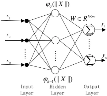
The model of Hermite neural network is shown in Figure 1. The model consists of input layer, hidden layer and output layer, where the input layer has n nodes

with T n

n R x x x

X =( ₁, ₂,..., ) ∈ as the input vector, the output layer has m nodes with T m

m R y y y

Y =( 1, 2,..., ) ∈

as the output vector. There are h hidden neurons which adopt a set of Hermite polynomials as activation functions. hm

R

W∈ × is the weight matrix from hidden layer to output layer, where

w

_jk is the connecting weight from jth _{node in hidden layer to k}th _{node in output layer.}

Σ

in the output layer nodes means that linear activation functions are used in the output layer neurons.

…… …… ……

∑

∑

||) (|| 0 X ϕ

||)

(||

1

X

h−

ϕ

m h R

W∈ ×

Figure.1. The model of Hermite neural network

Assuming there are P input vectors (X1_{, X}2_{, …… X}P_{) as}

learning samples and P output vectors (D1_,

D2, …… DP) as instructor signals. In order to build the functional mapping between input and output, Hermite Orthogonal basis functions are used to interpolate and approximate. The interpolation functions are defined as a linear combination of Hermite basis functions:

m k X w X F h j j jk

k( ) (|| ||) 1,2,..., 1

= =

∑

=

ϕ

(4)where ||X|| is a linear mapping Rn_→R.

C. Determination of Weights

Now, we discuss the iterative method and direct-determination method to obtain the weights of the network.

Theorem 2 The weights of Hermite neural network as shown in Figure 1 can be derived from the iterative formula as follow:

W(k+1) = W(k)- ηФT_{(ФW(k)-D) (5)}

where h P P h P P h h R X X X X X X X X X × − − − ∈ ⎥ ⎥ ⎥ ⎥ ⎥ ⎦ ⎤ ⎢ ⎢ ⎢ ⎢ ⎢ ⎣ ⎡ = Φ ||) (|| ||) (|| ||) (|| ||) (|| ||) (|| ||) (|| ||) (|| ||) (|| || (|| 1 1 0 2 1 2 1 2 0 1 1 1 1 1 0 ϕ ϕ ϕ ϕ ϕ ϕ ϕ ϕ ϕ " # % # # " "

and k = 0,1,2, ..., learning rate η should be small enough to ensure iterative convergence.

Theorem 3 (direct-weights-determination) The neural-weights of Hermite neural network could be obtained directly as formula:

D

W=(ΦTΦ)−1ΦT (6)

Where T T

pinv(Φ)=(Φ Φ)−1Φ is the pseudo inverse of Ф. Proof: According to Theorem 2, that is, W(k+1) = W(k)-

ηФT_{(ФW(k)-D). Since the learning rate η>0, so when the}

network reaches steady state (i.e., k is large enough), we will have W(k+1) = W(k) = W, which satisfy ФT_{(ФW-D) =}

0. Then we can use pseudo-inverse matrix and formula (6) to determine the optimal weights directly.

The Pseudo-inverse based direct-weight-determination for Hermite neural network avoids the lengthy iterative training, but can also achieve least square approximation for the mapping function between input and output. D. Adaptive Algorithm for Optimal Hidden-Layer

As we know, determination of the number of hidden neurons for neural network hidden layer is in the lack of theoretical guidance, and there is still no good method to determine network structure. Benefiting from the special structure of Hermite neural network, the optimal number of hidden neurons can be determined adaptively.

Given the target precision ε> 0 for the network, we can determine the minimum of hidden nodes to meet the requirement of precision adaptively as follows:

1) Initialize the number of hidden layer nodes as

1

+

+

=

n

m

h

, and set the target precision, such as ε

= 0.005;

2) Set the maximum of hidden nodes, such as MaxHideNode =

n

+

m

+

20

;

3) If h> MaxHideNode, it shows that the target precision can not be reached within MaxHideNode , and terminate the algorithm; otherwise, jump to step 4);

4) Use weights-direct-determination method to solve network optimal weights and then compute the current precision MSE(Mean Square Error);

5) if the MSE≤ε, it shows that the minimum of hidden layer nodes as h meeting the target precision requirement has been found, and terminate the algorithm. Otherwise set h = h + 1, jump to step 3).

The above algorithms can determine the minimum of hidden nodes speedily, and obtain the most simplified model structure of the neural network.

Ⅲ. ACQUISITION AND RECOGNITION OF DYNAMIC GESTUR

A. Extraction of gesture trajectory

To implement dynamic gesture recognition based on machine vision, the first work to do is to detect and track fingertips in real time, and obtain the gesture trajectory.

To simplify the tracking algorithm and improve the tracking efficiency, we propose an efficient method to detect and track fingertips based HSV color space as follows.

1) In order to reduce the effect of illumination, we employ H and S of HSV for learning the probability distribution of fingertip colors. A 2D color histogram is computed as the result of on-line training of fingertip colors. The 2D color histogram can be used as the basis of target fingertip detection and tracking;

2) Capture a video image, and convert the image from RGB to HSV;

3) Compute color probability distribution I(x, y) of the target through back-projection on the 2D color histogram;

4) Transform I(x, y) into a binary image B(x, y):

⎩ ⎨ ⎧

≥ < =

p y x I

p y x I y

x B

) , ( 1

) , ( 0 ) ,

( (7) where p is a given threshold.

5) Determinate the target region of fingertips through edge detection;

6) Determinate the centroid positions (xc,yc) of target

as follows:

∑∑

=

x y

y

x

B

M

₀₀

(

,

)

∑∑

=

x y

y

x

xB

M

₁₀

(

,

)

∑∑

=

x y

y

x

yB

M

₀₁

(

,

)

00 01 00

10

_,

M

M

y

M

M

x

c

=

c

=

(8)

7) Track the centroids of the fingertips through MDF(Minimum Distance First) , and go to step 2).

B. Model of dynamic gesture

Dynamic gestures are divided into two categories: four-finger-gesture (gesture with both hands) and two-finger-gesture (one hand gesture). For the four-finger-gestures such as zoom in, zoom out, rotation, etc, we can implement gesture recognition by analyzing the relative position of fingers of the left and right hand. In this paper, we focus on the recognition of two-finger-gesture.

TABLE I

The List of two-finger dynamic gestures

Gesture Interaction semantics Gesture stroke Digits Input digital number

。。。。。。

Confirm Confirm/Dial Cancel Cancel/Cancel the call Forward Forward/Scroll left

Backup Backward/Scroll right Pagedown Pagedown/Next sheet

PageUp Pageup/Previous sheet

So far, we have obtained a set of point for a two-finger-gesture (the mid-point of two fingertips)by fingertip tracking. If the set has more than 15 points, find the two points with minimum span, and replace them with their midpoint, repeat the operation until the number of the point in the set is 15. Then obtain 14 vectors by calculating the difference between two adjacent points and doing normalization, finally we can get the vector combination (28 components) of a two-finger-gesture. For example, the corresponding vector for number “6” gesture strokes as shown in figure 2 is:

{-0.93,0.36,-0.72,0.69,-0.47,0.88,-0.40,0.92,-0.26,0.97, -0.07,1.00,0.11,0.99,0.65,0.76,0.98,0.18,0.86,-0.51,0.46, -0.89,-0.49,-0.87,-0.98,-0.18,-1.00,0.00}.

Figure.2. The trajector of gesture “6” and its sample points

C. Dynamic gesture recognition based on Hermite neural network

1) The design of Hermite neural network structure The number of input nodes is set to 28, which is corresponding to the 28 components of gesture vector. The number of hidden nodes is set to 12 by means of the adaptive method discussed above to meet the requirement of precision 0.005. The number of output nodes must be compatible with the types of dynamic gestures to be recognized. As there are 16 types of gestures to be identified, we set the number of output nodes to 16.

2) Neural network training

We use 16X5 training samples for 16 types of gestures, that is, we use five training samples for each gesture.

For the input vectors of training samples, we can be obtained by the aforementioned method, and for the expected output vectors of training samples (teacher signal), as the gestures are divided into 16 types, so we use 16 unit vectors with length of 16 to represent these 16 gestures. An unit vector of which the mth _{element is 1 and}

the remaining elements are all 0 can be seen as the output of the mth _{gesture. For example, the expected}

output of the first gestuure “0” would be (1,0,0,0,0,0,0,0,0,0,0,0,0,0,0,0), and expected output of the fourteenth gestures “backward” would be (0,0,0,0,0,0,0,0,0,0,0,0,0,1,0,0).

The optical weight matrix W for Hermite neural network can be obtained through equation (6), and the trained Hermite neural network can be used for dynamic gesture recognition.

3) Identification of dynamic gesture

When the vector corresponding the dynamic gesture to be tested is input into the trained Hermite neural network, the gesture can be identified through the output of the network: the closer the output of the network approaching the predefined output of the Mth _{gesture, the more likely}

the input gesture is the Mth _gesture.

For example, the output of the network corresponding a input gesture is (0.01,0.00,0.00,0.00,0.01,0.00,0.00,0.00, 0.00,0.00,0.99,0.00,0.00,0.00,0.01,0.01), the maximum component is the 11th components, so we can determine that it is the gesture of No. 11, i.e. the gesture of “confirm”.

If the largest component of output vectors is less than a given threshold (e.g. 0.5), we can determine that the gesture is not a pre-defined gestures, that means gesture recognition fails.

dynamic gesture training and recognition for same samples.

A. Network training test

It can be seen from Table 2 that Hermite network is superior to BP neural network not only in training speed, but also in network precision. For Hermite network, the weights can be determined directly and the training time is

shortened to 0.57s, while for BP network trained by GDX and LM algorithm used in, the average training times were 15.3s and 6.5s. At the same time, The MSE of BP network trained by GDX and LM (setting the maximum of iterations to 3000 and target network performance to 0.005) are 0.0049925 and 0.0042041, while the MSE of Hermite networks is 0.0034623.

TableⅡ

Comparision of training results using Hermite network andtraditional BP network

Method Training process runtime(s) MSE

BP(GDX) 2213 iterations 15.30 0.0049925

BP(LM) 197 iterations 6.50 0.0042041

Hermite Network One step 0.57 0.0034623

B. Gesture recognition test

It can be seen from test result that Hermite neural network has novel robustness and generalization ability for dynamic gesture recognition to tolerate a certain range of gesture input differences. Part of the results are shown in Figure 3.

Figure.3. Robustness of Hermite network to gesture input

For each dynamic gesture, 200 samples were tested by Hermite neural network and BP neural networks trained by GDX and LM methods. The average accuracy of gesture recognition with BP trained by GDX and LM were 89.7% and 91.9%, while the average accuracy with Hermite neural network reached an average of 94.7%.

V. CONCLUSION

This paper construct a MIMO Hermite neural network for dynamic gesture recognition. Due to its direct-weights-determination and the adaptive algorithm to determine the number of hidden r nodes, it has overcome such shortcomings as slow convergence and low accuracy which exist in traditional BP networks, and greatly improved the training speed, and can meet the user’s requirement of performing online gesture training. At the same time, it improves the network accuracy and generalization ability significantly.

ACKNOWLEDGMENT

This work was supported by a grant from Natural Science Foundation of Guangdong, China (8152840301000009); Science and Technology Planning Project of Guangdong, China (2009B030803031).

REFERENCES

[1] Todd C. Alexander, Hassan S. Ahmed, Georgios C. Anagnostopoulos, “An Open Source Framework for Real-Time, Incremental, Static and Dynamic Hand Gesture Learning and Recognition”. Human-Computer Interaction,

Part II, HCII 2009, LNCS 5611, 2009: 123–130.

[2] Jos´e M. Moya, Ainhoa Montero de Espinosa, Alvaro Araujo,Juan-Mariano de Goyeneche, Juan Carlos Vallejo, “Low-Cost Gesture-Based Interaction for Intelligent Environments”. IWANN 2009, Part II, LNCS 5518, 2009:

752–755.

[3] Kaustubh, Sumantra, “Hand gesture modelling and recognition involving changing shapes and trajectories, using a Predictive EigenTracker”. Pattern Recognition Letters, 2007( 28): 329–334.

[4] Hardy Francke, Javier Ruiz-del-Solar, and Rodrigo Verschae, “Real-Time Hand Gesture Detection and Recognition Using Boosted Classifiers and Active Learning”. PSIVT 2007, LNCS 4872, 2007: 533–547.

[5] Jiyoung Park and Juneho Yi, “Efficient Fingertip Tracking and Mouse Pointer Control for a Human Mouse”．ICVS 2003, LNCS 2626, 2003: 88–97.

[6] Pang Zhonghua, Cui Hong, System Identification and Adaptive Control with MATLAB Simulation. Beijing：

BeiHang University Press, 2009.

[7] Martin T. Hagan, Howard B.Demuth, Mark H. Beale.

Neural Network Design. China Machine Press, 2002. [8] Wu Xiaojun, Wang Shitong, Yang Jingyu, Cao Qiying,

“The Study on the Orthogonal Polynomials-based Neural Networks and Its Properties”. Computer Engineering and Application，2002，38(9) :25-26.

[9] Jagdish C. Patra, Alex C. Kot. “Nonlinear Dynamic System Identification Using Chebyshev Functional Link Artificial Neural Networks”. IEEE TRANSACTIONS ON SYSTEMS, MAN, AND CYBERNETICS, PART B: CYBERNETICS, 2002, 32(4):505-511.

[10]Mu Li, Yigang He, “Nonlinear system identification using adaptive Chebyshev neural networks”. Intelligent Computing and Intelligent Systems (ICIS), 2010: 243- 247.

Chebyshev Basis Functions”. Computer Science，2009，

36(6): 210-213.

[12]ZHANG Yunong, CHEN Yangwen, YI Chenfu, LI Wei, “Feed-Forward Neural Network Activated with Hermite Orthogonal Polynomials and Its Weights-Determination Method”. Journal of Gansu Sciences,2008,20(1): 82-86.

Wensheng Li, born in 1966, M.S. associate professor. His

current research interest includes embedded software, biometrics, multimedia processing and communication.

Chunjian Deng, born in 1980, Ph.D. associate professor. His