An Optimized Algorithm for Reduce Task
Scheduling
Xiaotong Zhang
a, Bin Hu
b, Jiafu Jiang
ca,b,c School of Computer and Communication Engineering, University of Science and Technology Beijing , Beijing
100083, China
a Email: [email protected]
b,c Email:{hubin ustb, jiangjjf}@163.com
Abstract— In this paper, we propose a novel algorithm to
solve the starving problem of the small jobs and reduce the process time of the small jobs on Hadoop platform. Current schedulers of MapReduce/Hadoop are quite successful in achieving data locality and scheduling the reduce tasks with a greedy algorithm. Some jobs may have hundreds of map tasks and just several reduce tasks, in which case, the reduce tasks of the large jobs require more time for waiting, which will result in the starving problem of the small jobs. Since the map tasks and the reduce tasks are scheduled separately, we can change the way the scheduler launches the reduce tasks without affecting the map phase. Therefore we develop an optimized algorithm to schedule the reduce tasks with the shortest remaining time (SRT) of the map tasks. We apply our algorithm to the fair scheduler and the capacity scheduler, which are both widely used in real production environment. The evaluation results show that the SRT algorithm can decrease the process time of the small jobs effectively.
Index Terms— mapreduce, hadoop , schedule , SRT
I. INTRODUCTION
M
APREDUCE/ [1] is a programming model for processing large data sets on clusters of computers, the name of which is an implementation of the model by Google. A popular free implementation is Apache Hadoop [2]. Hadoop is a framework that allows for the distributed processing of large data sets across clusters of computers using simple programming models. Hadoop contains two important components: Hadoop Distributed File System (HDFS) and Hadoop MapReduce. HDFS provides a distributed, scalable filesystem for Hadoop. MapReduce is used for processing parallelizable problems across huge datasets using a large number of computers (nodes). The term MapReduce actually refers to two separate and distinct tasks that Hadoop programs perform. The map tasks take a set of data and convert them into another set of data, where individual elements are broken down into tuples (key/value pairs). The reduce tasks take the output from the map tasks as input and combine those data tuples into a smaller set of tuples. As the sequence ofManuscript received April 22, 2013; revised July 22, 2013; accepted August 27, 2013. c2005 IEEE.
This work was supported partially by National High-Tech Research and Development Program of China under Grant No.2011AA040101 and was jointly funded by the Fundamental Research Funds for the Central Universities China No.FRF-MP-12-007A.
the name MapReduce implies, the reduce tasks are always performed after the map tasks. In general, MapReduce framework contains a master node(JobTracker) and some slave nodes (TaskTracker). To process a job, the client submits a job to the JobTracker, which will do some initial work for the job and add the job to a queue. When a TaskTracker has the abilities to run tasks, it sends a request (heartbeat) to the JobTracker, which will use the TaskScheduler to pick up some tasks of the jobs in the queue, and assign them to the TaskTracker. The TaskTracker lives on each node of the Hadoop cluster and is responsible for executing tasks. The TaskTracker communicates with the JobTracker through a heartbeat protocol. In essence the heartbeat is a mechanism for the TaskTrackers to announce their availability on the cluster. In addition to announcing its availability, the heartbeat protocol also includes information about the state of the TaskTracker. Heartbeat messages indicate whether the TaskTracker is ready for the next task or not. When the JobTracker receives a heartbeat message from a TaskTracker declaring that it is ready for the next task, the JobTracker selects the next available job in the priority list and determines which task is appropriate for the TaskTracker to execute.
innate relation with the map phase, this can lead to poor utilization.
The reduce phase includes three subphases: shuffle, sort, and reduce. In the shuffle phase, input of a reduce task is the sorted output of the map tasks. In this phase the framework fetches the relevant partition of the output of all the map tasks, via HTTP. In the sort phase, the framework groups the inputs of the reduce tasks by keys (since different map tasks may have output the same key). The shuffle and sort phases occur simultaneously. As the map-outputs are being fetched, they will be merged momentarily. A reduce task copies all the data that belong to it from all map intermediate data, and sorts the data while copying. But it has to wait until all the intermediate data have been copied and sorted, then it begins the third stage. That means the real reduce function cannot start until all the map tasks are done. Some jobs may have hundreds of map tasks and just several reduce tasks, in which case, the reduce tasks may spend most of the time waiting for the data and keep occupying the resources. Therefore, this can lead to the starving problem of the small jobs [5].
Therefore, the role of a good scheduling algorithm is to efficiently assign each task to a priority to minimize makespan [6]. To solve this problem, Jian Tan et al. proposed a solution where the scheduler will gradually launch the reducer tasks depending on the map progress [7]. But it does not consider the factor of time. For example, a job with 80% map tasks completed may even has a longer time to finish all the map tasks than that of a job with only 20% map tasks completed. This thesis aims at providing a simple way of achieving launching the reduce tasks depending on the shortest remaining time (SRT) of the map tasks. In this way, we reduce the process time and the reduce time of the small jobs. We implement our algorithm based on the fair scheduler, which is widely used in real production environment. Our experiment results show that the reduce time of the jobs decreases a lot, especially for the small jobs (61%∼39 %). The process time of the small jobs can decrease by 55% at most. In addition, the process time of the large jobs can also decrease by 1% ∼ 4%. The remainder of this paper is organized as follows. In Section II, related work on different scheduling algorithms of Hadoop is presented. In Section III, the implement detail of the SRT algorithm and the drawback are described. In Section IV, the experimental results and the analyses of performance of the SRT scheduler on real Hadoop environment are given. Finally, in Section V, conclusions and suggestions for future work are presented.
II. RELATEDWORKS
In this section we briefly introduce some schedulers of Hadoop, including Hadoop inner schedulers (the FIFO scheduler, the fair scheduler, and the capacity scheduler) and schedulers developed by others. Specially, we focus on the fair scheduler.
A. FIFO scheduler
The FIFO scheduler is the default scheduler of Hadoop. In this scheduler, all jobs are submitted to a single queue, when a TaskTracker’s heartbeat comes, the scheduler simply picks up a job from the head of the queue, and tries to assign the tasks of the job, if the job has no tasks to be assigned (for example, all tasks have been assigned), then the scheduler tries the next job. The jobs in the queue are sorted by their priority, then submitted time.
The advantage of the FIFO scheduler is that the algo-rithm is quite simple and straightforward, the load of the JobTracker is relatively low. But it can result in starvation when the small jobs come after the large jobs. That means, a job has to wait until all the tasks (map, reduce) of the jobs before it have been launched.
B. Fair Scheduler
The fair scheduler is designed to assign resources to jobs such that each job gets roughly same amount of resources over time. For example, when there is only one job submitted, it uses the entire cluster, and when other jobs are submitted, tasks slots that free up are assigned to the new jobs. In this way, the problem of the FIFO scheduler that we mention above is solved: the small jobs can be finished in reasonable time while not starving the large jobs. The fair scheduler organizes jobs into pools and shares resources fairly across all pools. By default, each user is allocated a separate pool and gets an equal share of the cluster no matter how many jobs are submitted. Within each pool, either the fair sharing or the FIFO algorithm is used for scheduling jobs. In addition to providing fair sharing, the fair scheduler allows assigning guaranteed minimum shares to pools, which is useful for ensuring that certain users, groups or production applications always get sufficient resources. When a pool contains jobs, it gets at least its minimum share, however when the pool does not need its full guaranteed share, the excess is split between other pools. The fair scheduler implementation keeps track of the compute time for each job in the system. Periodically, the scheduler inspects the jobs to compute the difference between the compute time the job received and the time it should have received in an ideal scheduler. The result determines the deficit for the task. The fair scheduler will ensure that the task with the highest deficit is launched next. Disadvantages of the fair scheduler are listed below:
(1)The greed algorithm of launching reduce tasks will cause reduce starvation of the small jobs.
(2)Locality of the reduce tasks does not been consid-ered.
fair scheduler, which is widely used in real production environment. The detail of our algorithm is provided in section III.
C. Other schedulers
The capacity scheduler is designed to guarantee a minimum capacity of each organization. The central idea is that the available resources in the Hadoop cluster are partitioned among multiple organizations who collectively fund the cluster based on computing needs. In the capacity scheduler, several queues are created, each of which is assigned a guaranteed capacity (where the overall capacity of the cluster is the sum of each queue’s capacity). The queues are monitored, and if a queue is not consuming its allocated capacity, this excess capacity can be temporarily allocated to other queues. Given that the queues can represent a person or larger organization, any available capacity is redistributed for other users. To improve the data locality of the fair scheduler, Matei Zaharia et al. developed a simple technique called delay scheduling [8]. But it still ignored the locality of the reduce tasks. M. Hammoud et al. addressed this problem by incorporat-ing network locations and sizes of the partitions of the reduce tasks in the scheduling decisions, and mitigated network traffic and improved MapReduce performance [9]. Liying Li et al. [10] proposed a new improvement of the Hadoop relevant data locality scheduling algorithm based on LATE [11]. Besides, authors of [12] and [13] proposed schedulers which managed the jobs to meet deadlines. Similarly, the schedulers that were suitable for real-time circumstance were proposed [14] [15]. Sheng-bing Ren and Dieudonne Muheto proposed strategies to schedule tasks in OLAM (Online Analytic Mining) using MapReduce [16]. Specially, Xiaoli Wang et al. took full consideration of the relationship between the performance and energy consumption of servers, and proposed a new energy-efficient task scheduling model based on MapRe-duce, and gave the corresponding algorithm [17].
III. ALGORITHMDESCRIPTION
A. Algorithm Implement
Suppose we have M jobs waiting to be processed, we use J to represent the set of them.
J ={jobi|1≤i≤M} (1)
For everyjobi inJ, we represent the map tasks ofjobi byUi.
Ui=Fi∪Ri∪Pi (2)
The symbolsFi,Ri, and Pi represent the set of the fin-ished map tasks, the running map tasks, and the pending map tasks of jobi. In the fair scheduler, the pools are sorted by fair sharing algorithm while the jobs in a pool can be scheduled by either the FIFO algorithm or the fair sharing algorithm. We apply the SRT algorithm to the fair scheduler in this way: we change the way the fair scheduler sorts the jobs within a pool when scheduling the reduce tasks. To achieve that goal, we provide a
comparator called the SRT comparator to compare two jobs when sorting jobs according to their remaining time of the map tasks. To calculate the remaining time of the map tasks ofjobi, we have to estimate the remaining time of the tasks in bothRi and Pi. Let f(Ui) represent the remaining time it takes to finish all the tasks in Ui. We calculatef(Ui)like below:
f(Ui) =max[f(Ri), f(Pi)] (3) In fact, we have three methods to calculate f(Ri): we can treat the running tasks as the pending map tasks, or calculate the remaining time of each running task according to its progress and add them together, or we can simply ignore them. There is no mechanism through which we can obtain the process of a specified running task in Hadoop. Therefore, the second method will be difficult to achieve unless we modify the underlying architecture of Hadoop. Therefore we choose the third way to calculatef(Ui). Note that, two jobs with the same priority will have the same number of the running tasks according to the fair scheduler. Besides, each job will have a small and limited number of the running tasks when many jobs are processed simultaneously, in which casef(Ri)is much smaller thanf(Ui). Supposejobihas run for timeTi, the number of the finished map tasks is
fi, the number of the pending map tasks ispi,f(Ui)can be expressed like below:
f(Ui) =f(Pi) = (
+∞ fi = 0
Ti/fi∗pi fi 6= 0
(4)
We predict the remaining time of the map tasks in a job with the average time of map tasks multiplied by the amount of the pending map tasks. For example, suppose that a job has been running for 4 minutes, and it has 2 finished map tasks and 1 pending map task, we calculate the remaining time of the map tasks like this: 4 min / 2 * 1 = 2 min. Some other methods to estimate the remaining time of the jobs are provided in [18] [19] [20]. We let τs(i) and τe(i) represent the start time and end time ofjobirespectively, and letσs(i)andσe(i)represent the start time and end time of the reduce phase ofjobi respectively. Therefore,
AverageJ=
1
M
M X
i=1
[τe(i)−τs(i)] (5)
is the average process time of all jobs. And
AverageR=
1
M
M X
i=1
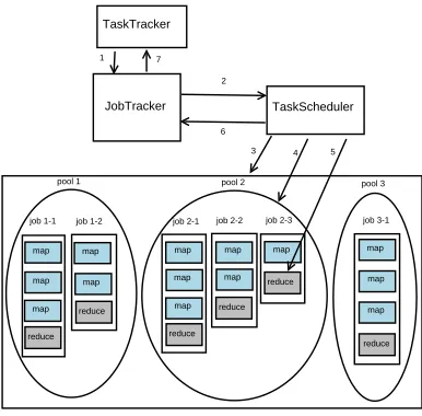
[σe(i)−σs(i)] (6) is the average process time of the reduce phases of all jobs. Once the request of a TaskTracker comes, we sort the jobs in the waiting queue, and assign tasks to the TaskTracker in order. The steps of assigning the reduce tasks using the SRT algorithm are shown in Fig. 1.
TaskTracker
JobTracker TaskScheduler
pool 1 pool 2 pool 3
job 2-1 job 2-2 job 2-3 job 1-2
job 1-1 job 3-1
map
map
map
map
map map
map map
map
reduce
reduce reduce
reduce map
map
reduce map
map
reduce map 1
2
3 4 5 6
7
Figure 1. The steps of assigning the reduce tasks
Step 2 The JobTracker forwards the request to the TaskScheduler.
Step 3 The TaskScheduler sorts the pools according to the fair scheduler. In this way the advantage of the fair scheduler can be achieved.
Step 4 The TaskScheduler selects a pool from the ordered pools (for example, pool 2), and sorts the jobs in pool 2 using the SRT algorithm.
Step 5 The TaskScheduler picks up a reduce task of the job with the shortest remaining time of the map phase.
Step 6 The TaskScheduler returns the reduce task to the JobTracker.
Step 7 The JobTracker assigns the reduce task to the TaskTracker.
The SRT comparator takes the status information of two jobs as input, and output an integer which indicates the order of two jobs. The detail of the SRT comparator is shown in Algorithm 1 below.
With the SRT algorithm, we make the reduce task of the shortest remaining time of the map phase get lanched before others. The remaining time of the map phase is changing dynamically according to the feedback. If two jobs both finish their map phases, we let the job with less map tasks lanch its reduce tasks ahead of another. Therefore, the small jobs will not be starving and the process time of the small jobs decreases greatly. The SRT algorithm focuses on scheduling the reduce tasks, therefore it can be easily applied to many other schedulers of Hadoop.
B. Drawback
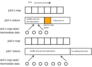
The SRT algorithm does not consider the time that the reduce tasks spend on the shuffle and the sort phases, which will sometimes lead to resource underutilization. For instance, if job1 has a shorter map remaining time than job2 does, we make job1 ahead of job2 according to the SRT algorithm. But if job2 has more intermediate data to copy, then it may be better to launch the reduce tasks
Algorithm 1 SRT comparator Require:
The status of two jobs(job1,job2):
fi : the number of the finished map tasks of jobi
pi : the number of the pending map tasks ofjobi
Ti : the time thatjobi has spent
Ensure:
-1 (schedule job1 prior job2);
0 (keep the current order of job1 and job2); 1 (schedule job2 prior job1).
1: iff1= 0∧f26= 0 then
2: return 1
3: else iff16= 0∧f2= 0then 4: return −1
5: else iff1= 0∧f2= 0then 6: ifp1> p2 then
7: return 1
8: else ifp1< p2 then 9: return −1
10: else
11: return 0
12: end if
13: else
14: ifp1= 0∧p2= 0then
15: iff1> f2 then
16: return 1
17: else iff1< f2 then
18: return −1
19: else
20: return 0
21: end if
22: end if
23: RemainingT ime1←T1/f1∗p1 24: RemainingT ime2←T2/f2∗p2
25: ifRemainingT ime1> RemainingT ime2then
26: return 1
27: else if RemainingT ime1 < RemainingT ime2
then
28: return −1
29: else
30: return 0
31: end if
32: end if
job1’s map
job1’s reduce
job1’s map tasks’ intermediate data
shuffle and sort the data below
wait for map phase
reduce go on Time
job2’s map
job2’ reduce
job2’s map tasks’ intermediate data
shuffle and sort the data below no waiting time here
Figure 2. Consider the shuffle phase and the sort phase
TABLE I.
THE HARDWARE CONFIGURATION
No. Type CPU Memory
0 Master 8-core, 2.13GHz 16G 1 Slave 4-core, 2.13GHz 4G 2 Slave 4-core, 2.13GHz 4G 3 Slave 8-core, 2.13GHz 16G 4 Slave 8-core, 2.13GHz 4G 5 Slave 16-core, 2.66GHz 48G 6 Slave 16-core, 2.66GHz 48G 7 Slave 16-core, 2.66GHz 48G 8 Slave 4-core, 2.13GHz 4G 9 Slave 4-core, 2.13GHz 4G 10 Slave 4-core, 2.13GHz 4G
jobs.
IV. EXPERIMENT ARESULTS
In order to evaluate the performance of the SRT al-gorithm, we conduct a series of experiments. We use gridmix2 as a tool to make the tests. Gridmix2 is a benchmark of Hadoop. It can automatically generate and submit some jobs, which can be configured in the kind and the amount of the reduce tasks. There are two kinds of jobs in our experiments: small and large. The large jobs have more map tasks and will take a longer time to finish their map phases. Without loss of generality, we firstly submit all the jobs with random order. We compare the average reduce time, average job process time, and the total time for finishing all the jobs using both the SRT algorithm and the fair scheduler on our test bed. We repeat each test for twenty times. Secondly, we conduct an experiment in which jobs are submitted with the order from large ones to small ones. In this way we can find out how the algorithm works in the worst situation. Thirdly, we repeat the first experiment under different number of slave nodes. Finally, we apply the SRT algorithm to the capacity scheduler. The hardware configuration in our experiments is showed in Table I.
A. Random Order
In this experiment, we submit the jobs by a random program. The test bed that we use contains five nodes: No.0 ∼ No.4. We conduct four groups of tests, each group has a different amount of jobs, while the numbers of different kinds (small, large) of jobs in the same group
m m
Figure 3. The process time of the small jobs
m m
Figure 4. The process time of the large jobs
are the same. Each group has 10×2, 20×2, 30×2,
40×2jobs respectively. For example the first group will have 10 small jobs and 10 large jobs. The tests in each group will be repeated for twenty times. Figure [3, 4] show the results of the average job process time of two kinds of jobs when using the SRT scheduler and the fair scheduler.
It is clear that the process time of the small jobs can decrease effectively when using the SRT algorithm. When the number of jobs is not that large (10×2), the process time of the small jobs can even decrease by 55%. Figure 4 shows that the process time of the large jobs keeps nearly the same using two different schedulers. The process time of large jobs can decrease by 1% ∼ 4%. We can see that the SRT algorithm has different effects on different jobs because it has different effects on reducing the process time of the reduce tasks. To see whether the SRT algorithm really has an influence on the reduce phase, we calculate the average reduce time of the jobs, figure [5, 6] show the results.
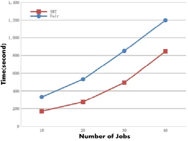
The reduce time of both small jobs and large jobs decreases. Specially, the reduce time of the small jobs gets a decrease of 61% to 39%. Figure 7 shows the compare of the process time total jobs.
The process time of total jobs is determined by when the last job finishes. We can see that the process time of total jobs of the SRT algorithm is a little more than that of the fair scheduler. For example, when we submit40×2
m m
Figure 5. The reduce time of the small jobs
m m
Figure 6. The reduce time of the large jobs
is 6% more than that of the fair scheduler. This may be due to the large jobs being pushed behind the small jobs and taking a longer time to finish.
B. Small jobs come after large jobs
In this experiment, we submit all small jobs after large jobs. The test bed contains one master node (No.0) and four slave nodes(No.1∼No.4). We submit 10 large jobs, wait for 5 seconds, and then submit 10 small jobs. The time interval between two submission is used to ensure that the jobs submitted earlier can be initialized before those submitted later so that all the jobs are in the right order we want. Figure 8 shows the results of the average job process time of two kinds of jobs.
m m
Figure 7. The process time of total jobs
Figure 8. The job process time when the small jobs come after the large jobs
m mm
Figure 9. The job process time of the small jobs under different number of slave nodes
We can see that the small jobs can get 39% decrease of process time with the SRT algorithm. And the job process time of the large jobs is nearly the same under two schedulers.
C. Scalability
In this experiment, we repeat the first experiment under different number of slave nodes to see the scalability of the SRT scheduler. We conduct four groups of tests, each group has 4, 6, 8, 10 slave nodes respectively. For example, in the fourth group of tests, the test bed contains one master node (No.0) and ten slave nodes(No.1 ∼ No.10). In each test we submit 40 small jobs and 40 large jobs. Each group of tests are repeated for twenty times. Figure [9,10] show the results of the average job process time of two kinds of jobs.
m mm
Figure 10. The job process time of the large jobs under different number of slave nodes
m m
Figure 11. The process time of the small jobs
D. Apply the SRT algorithm to the capacity scheduler
The capacity scheduler is another popular scheduler of Hadoop, and we apply the SRT algorithm to it and see how it can reduce the process time of the small jobs. As we see from the scenario of Fig. 11, the SRT algorithm can perfectly reduce the process time of the small jobs when working with the capacity scheduler.
V. CONCLUSIONS
In this paper, we propose a simple algorithm for scheduling the reduce tasks based on the shortest remain-ing time of the map tasks. We implement our algorithm by applying the SRT algorithm to the fair scheduler and the capacity scheduler, which have been proved by several experiments. The results of the experiments show that the SRT algorithm decreases the reduce time and process time of the small jobs without affecting the performance of large jobs. However, the process time of total jobs of the SRT scheduler is a little more than that of the fair scheduler. In the future, we will improve our algorithm by considering the time of the reduce phase and using a more precise method to estimate the remaining time of both the map and the reduce phases. We also plan to consider several high-level objectives, such as the intelligent scheduler based on genetic algorithm and energy saving.
ACKNOWLEDGMENT
This work was supported partially by National High-Tech Research and Development Program of China under Grant No.2011AA040101 and was jointly funded by the Fundamental Research Funds for the Central Universities China No.FRF-MP-12-007A.
REFERENCES
[1] J. Dean and S. Ghemawat, “Mapreduce: simplified data processing on large clusters,” Commun. ACM, vol. 51, no. 1, pp. 107–113, Jan. 2008.
[2] “Apache hadoop,” http://hadoop.apache.org.
[3] “Fair scheuler,” http://hadoop.apache.org/docs/r1.0.4/fair scheduler.html.
[4] “Capacity scheduler,” http://hadoop.apache.org/ mapreduce/docs/r0.21.0/capacityscheduler.html.
[5] J. Tan, X. Meng, and L. Zhang, “Delay tails in mapreduce scheduling,” in Proceedings of the 12th ACM SIGMET-RICS/PERFORMANCE joint international conference on Measurement and Modeling of Computer Systems, ser. SIGMETRICS ’12. New York, NY, USA: ACM, 2012, pp. 5–16.
[6] Y. Xu, K. Li, T. T. Khac, and M. Qiu, “A multiple priority queueing genetic algorithm for task scheduling on heterogeneous computing systems,” Liverpool, United kingdom, 2012, pp. 639 – 646.
[7] J. Tan, X. Meng, and L. Zhang, “Coupling scheduler for mapreduce/hadoop,” in Proceedings of the 21st in-ternational symposium on High-Performance Parallel and Distributed Computing, ser. HPDC ’12. New York, NY, USA: ACM, 2012, pp. 129–130.
[8] M. Zaharia, D. Borthakur, J. Sen Sarma, K. Elmeleegy, S. Shenker, and I. Stoica, “Delay scheduling: a simple technique for achieving locality and fairness in cluster scheduling,” in Proceedings of the 5th European confer-ence on Computer systems, ser. EuroSys ’10. New York, NY, USA: ACM, 2010, pp. 265–278.
[9] M. Hammoud and M. Sakr, “Locality-aware reduce task scheduling for mapreduce,” in Cloud Computing Technol-ogy and Science (CloudCom), 2011 IEEE Third Interna-tional Conference on, 29 2011-dec. 1 2011.
[10] L. Li, Z. Tang, R. Li, and L. Yang, “New improvement of the hadoop relevant data locality scheduling algorithm based on late,” in Mechatronic Science, Electric Engineer-ing and Computer (MEC), 2011 International Conference on, aug. 2011, pp. 1419 –1422.
[11] M. Zaharia, A. Konwinski, A. D. Joseph, R. H. Katz, and I. Stoica, “Improving mapreduce performance in heteroge-neous environments.” in OSDI, vol. 8, no. 4, 2008, p. 7. [12] K. Kc and K. Anyanwu, “Scheduling hadoop jobs to meet
deadlines,” in Cloud Computing Technology and Science (CloudCom), 2010 IEEE Second International Conference on, 30 2010-dec. 3 2010, pp. 388 –392.
[13] L. Liu, Y. Zhou, M. Liu, G. Xu, X. Chen, D. Fan, and Q. Wang, “Preemptive hadoop jobs scheduling under a deadline,” in Semantics, Knowledge and Grids (SKG), 2012 Eighth International Conference on, 2012, pp. 72–79. [14] X. Dong, Y. Wang, and H. Liao, “Scheduling mixed real-time and non-real-real-time applications in mapreduce environ-ment,” in Parallel and Distributed Systems (ICPADS), 2011 IEEE 17th International Conference on, 2011, pp. 9–16. [15] L. Phan, Z. Zhang, Q. Zheng, B. T. Loo, and I. Lee, “An
[16] S. Ren and D. Muheto, “A reactive scheduling strategy applied on mapreduce olam operators system,” Journal of Software, vol. 7, no. 11, pp. 2649–2656, 2012.
[17] X. Wang, Y. Wang, and H. Zhu, “Energy-efficient task scheduling model based on mapreduce for cloud com-puting using genetic algorithm,” Journal of Computers (Finland), vol. 7, no. 12, pp. 2962 – 2970, 2012. [18] J. Polo, D. de Nadal, D. Carrera, Y. Becerra, V. Beltran,
J. Torres, and E. Ayguad´e, “Adaptive task scheduling for multijob mapreduce environments,” 2009.
[19] Z. Tang, J. Zhou, K. Li, and R. Li, “Mtsd: A task scheduling algorithm for mapreduce base on deadline constraints,” in Parallel and Distributed Processing Sym-posium Workshops PhD Forum (IPDPSW), 2012 IEEE 26th International, may 2012, pp. 2012 –2018.
[20] S. BARDHAN and D. MENASC, “Queuing network mod-els to predict the completion time of the map phase of mapreduce jobs,” 2012.
[21] H. Chang, M. Kodialam, R. Kompella, T. Lakshman, M. Lee, and S. Mukherjee, “Scheduling in mapreduce-like systems for fast completion time,” in INFOCOM, 2011 Proceedings IEEE, april 2011, pp. 3074 –3082.
Xiaotong Zhang received the M.S., and Ph.D. degrees from
University of Science and Technology Beijing, in 1997, and 2000, respectively. He was a Professor in the Department of School of Computer and Communication Engineering, Uni-versity of Science and Technology Beijing, from 2000 to 2013. He was as a visiting scholar supervised by Prof. Liang Cheng in LONG Lab of Deportment of Computer Science and Engineering of Lehigh University during 2010. His industry experience includes affiliation with Beijing BM Electronics High-Technology Co., Ltd. from 2002 to 2003, where he worked on digital video broadcasting communication systems and IC design, His industrial cooperation experience includes BLX IC Design Co., Ltd, NorthCommunications Corporation of PetroChina, and Huawei Technologies Co., Ltd.Etc. His research includes work in quality of wireless channels and networks, wireless sensor networks, networks management, cross-layer design, resource allocationof broadband and signal processing of communication.
Bin Hu is a student of School of Computer & Communication
at University of Science and Technology Beijing. He pursued his Ph.D. in the field of Cloud Storage platforms and Massive Data Mining.
Jiafu Jiang is currently a graduate student and working towards