ISSN (Online): 2320-9364, ISSN (Print): 2320-9356
www.ijres.org Volume 1 Issue 4 ǁ August. 2013 ǁ PP.31-37
Method of Adaptive Forecasting Based On Multidimensional
Linear Extrapolation
Mantula E.V.
1, Mashtalir S.V.
1 1(Informatics department, Kharkiv National University of Radio Electronics, Ukraine)
ABSTRACT:
The paper is sanctified to the problem of time series analysis. The linear extrapolation methods of multidimensional time series with Euclidian metric and proximity function is offered. As practical application the problem of spatio-temporal segmentation of video is considered.Keywords –
linear extrapolation, multidimensional, time series, metric, videoI.
INTRODUCTION
A necessity of forecasting time series heterogeneous in nature often arises for different applications, viz. technical, financial, economic, medico-biological, environmental, agricultural ones, etc. Nowadays, there exists a variety of methods to solve such problems: from traditional statistical and adaptive [1-5] approaches to more sophisticated techniques with artificial neural networks in use [6-10].
More complicated situation appears when a predicted sequence is multidimensional. However, this problem can also be solved either by decomposition of the original multidimensional series to the set of one-dimensional ones or by means of multi-one-dimensional (MIMO) predictive models which parameters can be successfully identified by the same statistics, adaptive or neural network algorithms.
It should be emphasized that successful application of these procedures assumes availability of sufficiently representative sample of observations, which gives possibility to create a fairly accurate predictive model. Unfortunately, often there are situations when the sample is either small or predictable process is not stationary, so its prehistory cannot be used to find parameters of the model. It is very hard to think about effective predictive model in this situation and therefore, prediction methods should be introduced, that do not use the concept of the model. Such approach becomes especially important when it is required to process enormous data volumes on-line or even in real time, e.g. its application to shot (basic unit of video content analysis) boundary detection for video annotation and retrieval due to inherently temporal aspect of video streams. The key to explaining this fact may lie in that content-based video retrieval systems have become an active field of research along with both the rapid increase in the amount of video acquisition and wide range of video applications, what is additionally emphasized by arbitrariness of video structures and semantic concepts. In any case, shot boundary detection can be a ground for effective parsing, as time series processing is an essential component of preliminary video analysis and forecasting.
The paper is devoted to the development and improvement of one of the possible approaches to multidimensional time series forecasting. The structure of the paper is as follows. The second section sketches multidimensional linear extrapolation problem. Section 3 enlarges upon an adaptive multidimensional linear extrapolation algorithm with Euclidean metric. Section 4 presents a new algorithmic approach to the adaptive multidimensional linear extrapolation based on the proximity function. The final section proposes summarized results.
II.
The method of multidimensional linear extrapolation
The basis of traditional mathematical forecasting methods (statistical, adaptive, neural networking, etc.) consists in different kinds of mathematical models obtained as a result of structural and parametric identification. Problems of time extrapolation are usually solved on the basis of mathematical models, and such models explicitly or implicitly include discrete time as an argument. Predictive model synthesis is not possible if there is not enough data to construct the mathematical model. In this case, spatial prediction (extrapolation) can be used instead of time extrapolation, which comes to estimation of vector field under particular observations. Multidimensional linear extrapolation [11] should be marked among the most promising methods of spatial extrapolation, it has proved its effectiveness for solving some actual design problems and control of complex multi-dimensional nonlinear objects. Consider multidimensional linear extrapolation method applied to the problem of one-step prediction of n-dimensional nonlinear nonstationary time series y k k( ), 1, 2,...,N where
, 1 1
2 2
ˆ ( ) ( ( 1),..., ( ), ( 1),..., ( ),
( 1),..., ( ),..., ( ),..., ( ))
i i i i A i B
B p q B
y k f y k y k n x k x k n
x k x k n x k l x k n
, ,
1 , ,
( ( ),..., ( ),..., ( )) ,
A B
A i i q
i i i n i n n
f z k z k z k
(1)
where fi( ) is a priori unknown nonlinear relation which should be restored from available observations; y kˆ ( )i
stands for an evaluation (prediction) of the controlled sequence y ki( ), performed using data available by
(k1) point in time; i1,..., ;n nA i, denotes the considered history depth of the analyzed sequence (generally
A, B
n n are memory parameters of observations); xp(kl) is p-th exogenous component of multidimensional
signal that affects y ki( ); l1,...,nB; p1,...,q. Expression (1) can also be rewritten in vector-matrix form
ˆ( ) ( ( 1),..., ( A), ( 1),..., ( B)) ( ( ))
y k F y k y kn x k x kn F z k (2)
where y kˆ( )(y k y kˆ1( ),ˆ2( ),...,yˆn( ))k T, y k( )(y k1( ),...,yn( ))k T, x k( 1) ( (x k1 1),...x k lq( ))T,
( ) ( T( 1),..., T( A), T( 1),..., T( B))T
z k y k y kn x k x kn is (n n AqnB) 1 prehistory vector.
Non-linear transformations fi( ) and F( ) can be retrieved in the process of any artificial neural network learning when a learning sample exists. However, if the sample is small enough, the neural network approach is unusable, while multivariate linear extrapolation will provide quite accurate results. The problem of multidimensional linear extrapolation applied to prediction of multidimensional time series can be described using notations (1), (2) as follows [11]. Let matrix of precedents (prehistory)
(1), (1)
(2), (2)
( ), ( )
T T
T T
T T
z y
z y
z N y N
be defined with dimension N(nnAqnBn). Extrapolation, in fact, is reduced to evaluation of
ˆ( 1) ( ( 1), )
y N z N , (3) in time point N, where ( ) is extrapolation algorithm which should meet a number of requirements. The main requirement is that after its application, all the consequences matrix of precedents should be accurately recovered, i.e.
ˆ( ) ( ) ( ( ), )
y k y k z k , k1, 2,...N. (4) It should be noted that prediction methods based on various mathematical models almost never provide the condition (4). From the other requirements it can be noted that the algorithm ( ) should be constructed in a vector form, i.e.
1
( ,..., n)
, yi
i( , )Z , i1,...,n; (5) the complexity should increase by n and N not faster than linearly; the algorithm must be able to operate for all N (even if N1). It is clear that for small N, and also N1, sufficiently accurate mathematical model cannot in principle be constructed.III.
An adaptive multidimensional linear extrapolation algorithm with Euclidean metric
According to L.A. Rastrigin [11], consider multidimensional linear extrapolation algorithm as the following sequence of steps:i). generation of predicted process history in the form of matrices
( (1), (2),..., ( ))
Z z z z N is matrix of (nnAqnB)N dimension,
( (1), (2),..., ( ))
Y y y y N is n N matrix;
ii). finding the weight vector ( 1, 2...,N)T that provides minimum for norm function
2 2
1
|| (z N 1)
kN
( ) ( )||k z k Z N( 1) Z
; (6) iii). formation of optimal prediction as a linear combination1
ˆ( 1) ( )
N k k
y N y k Y
. (7)as a result, it is obvious that
1
(Z ZT ) Z z NT ( 1)
(8)
which exists only if the matrix Z ZT is nonsingular. It is essential to see that under sufficiently small N
(NnnAqnB) this is not true, therefore it is proposed to use pseudoinverse matrix [12] and finally we have the expression
( 1) Z z N
(9) from which it follows that, in fact, the problem is reduced to finding orthogonal projection of the vector
( 1)
z N on the linear hull generated by the prehistory vectors Z .
From computational point of view there are no difficulties in the implementation of this procedure, however, the solution becomes more complicated if the processing data are sequential in real time. In this case, all previous relations can be rewritten in the following form
( (1), (2),..., ( )) k
Z z z z k ,
( (1), (2),..., ( )) k
Y y y y k ,
2 2
1
|| (z k 1)
lklz l( )|| || (z k 1) Zkk|| , (10)1 2
( , ,..., )T
k k
,
1
ˆ( 1) ( )
k
l k k
l
y k y l Y
, (11)( 1)
k Z z kk
. (12)
In [11] it is proposed to use Greville formulae for the matrix Zk1 calculation from available Zk and incoming values z k( 1), y k( 1), although it is much more preferable to replace it by regularized version of (8) in the form
1
( T ) ( 1)
k Z Zk k Ik Z z kk
(13) where
is regularization parameter, Ikdenotes (k k ) identity matrix.For processing of non-stationary time series, which characteristics change unpredictably over time, it is appropriate to solve the problem in the ‘sliding window’ instead of all available sample processing. ‘Sliding window’ consists of
most recent observations, and in this case relations (10) – (12) can be rewritten as follows, ( ( 1), ( 2),..., ( ))
k
Z z k z k z k ,
, ( ( 1), ( 2),..., ( ))
k
Y y k y k y k ,
2 2
, ,
1
|| (z k 1)
l kk
lz l( )|| || (z k 1) Zkk|| , (14), ( 1,..., )T
k
k
k ,
, , 1
ˆ( 1) ( )
k
l k k
l k
y k y l Y
, (15), , ( 1)
k Zkz k
. (16)
For implementation of this procedure in real time, the recurrent algorithm of pseudoinversion on ‘sliding window’ had been proposed in [11], but it is inconvenient and computationally complex. In this regard it is expedient to use a modification of (13) in ‘window’ view, and its packet form can be written as
1
, ( T, , ) , ( 1)
k ZkZk
I Zkz k , (17)
. 1, ,
1 0,
( )( ( 1) ( )) ( ), 1 ( ) ( ) ( )
( 1) ( ) ( ) ( 1)
( 1) ( 1) ,
1 ( ) ( 1) ( ) ( 1) ( ) ( ) ( 1)
( ) ( 1) ,
1 ( ) ( 1) ( ) 0, ( ) .
T k
k k T
T
T
T
T
k z k z k
z k
z k k z k
k z k z k k
k k
z k k z k
k z k z k k
k k
z k k z k
k I (18)
Actually the forecast is calculated according to (15).
It is evident that expressions (15), (18) simplify prediction considerably, but there arises a question of reasonable choice of window
size which is usually specified by some heuristics, that in the end reduces the overall efficiency of the approach.IV.
Adaptive method of multidimensional linear extrapolation based on the proximity
function
Multi-dimensional extrapolation method proposed below is based on the proximity (distance) between the last history vector z N( 1) and all previous data z(1),.., ( )z N , and also it is based on making predictions
ˆ( 1)
y N using the same function.
Implementation of the method consists in the following steps:
i). Calculation of the distance between the vector z N( 1) and all the previous functions z k( ) on the basis of proximity function d N( 1, )k (in the simplest case, this is the Euclidean metric)
( 1, ) || ( 1) ( )||
d N k x N x k k;
ii). Arrangement of these distances in increasing order (ranking)
1 2
1 2
( 1, ) ( 1, ) ... N( 1, N) d N k d N k d N k ;
iii). Selection of the first
vectors, for which the following condition is true( 1, )
d N k
where is given or computed threshold; iv). Finding a set of weights l
1 1 1 ( ) ,1 ( ) l l l l d l d
;v). Forecast computing
1
ˆ( 1) l ( )
l
y N z l
.All iterations are repeated under acquisition of a new experimental observation y N( 1).
Thus,
observations are also involved at each step of forecast formation, but this value may change,and it is clear that the less
is, the more non-stationary the signal is. It is also easy to see that ify k( )const, then
N, l 1N
.One of the issues that can be solved with the above mentioned forecasting approach is video analysis. This is mostly due to multidimensional time series nature of video data. Besides, one of the peculiarities common for video data should be noted. It consists in close similarity of consecutive video frames (from a single shot), which permits forecasting future frames based on the previous ones. In particular, this video property is often used in a number of compression algorithms. For shot boundary detection, where a search for fragments with a common sense is an issue, video segmentation should be considered.
In order to extract segments with a common sense from initial data, it is possible to use the aforementioned approach in a following way: if the forecast (15) for N1 frame differs significantly from its actual value, it should be interpreted as a change of a shot, and consequently as a segment boundary. By doing so, the forecast may be performed only for vectors included into a single segment, otherwise values from the previous video segments may give a negative impact on the whole process of segmentation. Thereby, extrapolation intervals should be shifted according to segment boundaries while making forecasts.
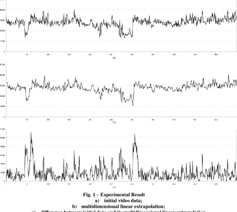
Fig. 1 shows an example of video application for the proposed extrapolation method. It can be seen clearly that the moment when characteristic values change a lot over a period, the forecast also changes greatly in some time. In other words, the difference between an actual value and its forecast defines moments of changes in shots. In addition, if short-term random outliers appear, they are smoothed, and they do not influence shot boundary detection.
Fig. 1 – Experimental Result a) initial video data;
b) multidimensional linear extrapolation;
c) difference between initial data and itsmultidimensional linear extrapolation
Using this line of reasoning, one may come to the conclusion that the proposed extrapolation approach can be used for «rough» temporal partitioning in terms of spatio-temporal segmentation.
V.
CONCLUSION
to make pseudoinversion. It is rather simple from computational point of view.
However, when choosing forgetting parameter, smoothing effect can affect forecasting validity, and it is required to take into consideration assessment of both threshold and length of ‘sliding window’. It is known with certainty that there is a good reason to create procedures of finding these parameters which ought to be included in adaptive forecasting based on multidimensional linear extrapolation.
References
[1] G.E.P. Box, G.M. Jenkins, G.C. Reinsel, Time Series Analysis: Forecasting and Control. 4th Edition (Inbunden: Wiley Series in Probability and Statistics, 2008).
[2] S. Makridakis, S. Wheelwright, R.J. Hyndman, Forecasting: methods and applications (New York: John Wiley & Sons, 1998).
[3] D.C. Lewis, Industrial and Business Forecasting Methods. (London: Butterworths Scientific, 1982) [4] T. Masters, Neural, Novel & Hybrid Algorithms for Time Series Prediction (N.Y.: John Wiley & Sons,
Inc., 1995).
[5] Yu.P. Lucashin, Adaptive methods of short-term prognosis of time series (М.: Finance and statistics, 2003). /In Russian/
[6] A.G. Ivachnenko, J.A. Muller, Selbstorganization von Vorherzagemodellen (Berlin: VEB Verlag Technik, 1984).
[7] D.T. Pham, X. Liu, Neural Networks for Identification, Prediction and Control (London: Springer – Verlag, 1995).
[8] S. Kingdom, Intelligent Systems and Financial Forecasting. (Berlin: Springer – Verlag, 1997).
[9] J.S. Zirilli, Financial Prediction Using Neural Networks (London: Int. Thomson Computer Press, 1997).
[10] D.P. Mandic, J.A. Chambers, Recurrent Neural Networks for Prediction (Chichester: John Wiley & Sons, Ltd., 2001).
[11] L.A. Rastrygin, Yu.P. Ponomariov, Extrapolation methods in planning and management (M.: Engineer, 1986). /In Russian/
[12] А. Аlbert, Regression and the moor-penrose pseudoinverse (N.Y. and London: Academic Press, 1972). [13] Ye. Bodyanskiy, O. Rudenko, Artificial neural networks: architectures, educating, application
(Kharkov. TELETECH, 2004). /In Russian/