A Distributed AOA Based Localization
Algorithm for Wireless Sensor Networks
Gabriele Di Stefano, Alberto Petricola
Department of Electrical and Information Engineering, University of L’Aquila, Italy Email:{gabriele,petricol}@ing.univaq.it
Abstract— In this paper we propose a distributed algorithm
for solving the positioning problem in ad-hoc wireless networks. The method is based on the capability of the nodes to measure the angle of arrival (AOA) of the signals they produce. The main features of the distributed algo-rithm are simplicity, asynchronous operations (i.e. no global coordination among nodes is required), ability to operate in disconnected networks. Moreover each node can join the computation at any time. Numerical results, obtained by simulating several scenarios, show that the algorithm can reach a good level of convergence even when the number of communications is limited.
Index Terms— distributed algorithm, sensor networks, angle
of arrival
I. INTRODUCTION
Ad-hoc wireless networks consisting of sensor and actuator nodes are typically proposed for monitoring and controlling environmental characteristics (such as light, temperature, sound, and many others) in many attractive applications. Most of involved data are useful only when associated to the geographic location of nodes. Hence, most sensor data are required to be stamped with position information. However, acquiring this position data can be quite challenging. GPS (Global Positioning System) can satisfy some of the requirements, but attaching a GPS receiver to each node is a quite costly (in volume, money, and power consumption) solution. Moreover, GPS reception might be obstructed by climatic conditions, or impractical in indoor environments, and even with the selective availability recently turned off, the location error might still be of 7-10m, which might be larger than the hop size of some networks. The same consideration are valid also for systems like FCC Enhanced 911 [1], which enables emergency services to locate geographic positions of cellular wireless callers, whose phase II achieves a localization accuracy within 50 to 300 m.
A consequence of the ad-hoc nature of these networks is the lack of infrastructure inherent to them. With very few exceptions, all nodes are considered equal, but we can assume the presence of some anchor nodes. An anchor node is a node that is given a priori knowledge of its posi-tion with respect to some global coordinate system. The positioning problem consists in calculating the position of non-anchor nodes, exchanging informations between neighboring nodes.
There are several requirements a positioning algorithm has to satisfy (see [2]) in the depicted context. Firstly,
it should be distributed: in a very large network of miniaturized nodes, designed for intermittent operation, even shuttling the entire topology to a server in a hop by hop manner would put too high a strain on the nodes close to the server. Partitioned areas would make centralization impractical, and anisotropic networks would put more strain on some nodes. Changing topologies would also make the centralized solution undesirable. Second, the algorithm has to minimize the amount of node-to-node communication and computation power, as the radio and the processor are the main sources of draining battery life. Third, the positioning system should work even if the network becomes disconnected - in the context of sensor networks, the data can be later collected by a fly-over basestation. Finally, it is desirable to provide absolute positioning, in the global coordinate system of the GPS, as opposed to relative coordinates, since relative positioning might incur a higher signaling cost in the case the network topology changes, and absolute positioning enables a unique name-space, that of GPS coordinates.
Our algorithm is distributed, robust against disconnec-tion, and provides absolute positions in a global coor-dinate system. Its communication load, even if slightly greater with respect to a centralized solution, is main-tained limited and equally distributed among nodes through a careful, consumption-aware implementation.
Related works: There are several approaches to face the positioning problem without the use of any infrastructure in sensor networks. Range-free approaches use only the connectivity between nodes [3]–[5]. These methods are almost insensitive to measurement noises, but a high node density is required to achieve accurate location estimation.
Range-based approaches measure the proximity (in terms of hop-count or estimated distance) to a few land-marks with known locations [2], [6]–[13]. When a node has measured the distances to its neighbors, it broadcasts this information. This allows for the construction of (partial) local maps with relative positions. Adjacent local maps are combined by aligning (mirroring, rotating) the coordinate systems. These proposals work well in the isotropic space but their performance severely degrades in anisotropic indoor environments. Due to the importance of these techniques, many efforts have been devoted to the study of the location error characteristics arising in this context (see, e.g., [14]–[16]).
the nodes to sense the direction from which a signal is received, which is known as angle of arrival (AOA). This approach has been considered in the work by Niculescu and Nath [17], in which two algorithms (called DV-Bearing and DV-Radial) are developed to infer node positions. Recent works use AOA combined with rang-ing [18], [19]: the limitation of this approach is in the technical difficulties to build nodes with both measure-ment capabilities.
Theoretical studies in [20] show that the localization problem based on AOA is NP-complete.
This work: We re-consider the AOA approach in this paper, proposing a distributed algorithm, where each node can perform an estimation of its location by knowing the estimated positions of nodes that fall into its transmission range, and by measuring angles of arrival. The behavior of each node is such that the overall computation solves a least squares problem in order to reduce the differences among the actual positions and the estimated ones. This approach is similar to that in [21] where the authors proposed a range-based positioning algorithm.
What makes our algorithm also different from the algorithm proposed in [17] is that there are no multihop phases which imply an implicit sequencing of the overall calculation. Calculations are only based on difference of angles of arrival, making localization independent from heading sensing (no compass is needed both by anchor and non-anchor nodes). Moreover, it does not force any serial computation between pairs of nodes and, as conse-quence, new nodes, or nodes with intermittent behavior, can join the network at any time.
Our algorithm requires AOA sensing capability and then either an antenna array, or a small set of ultrasound receivers at each node. Small form factor nodes with these characteristics have been developed by the Cricket Compass project [22] from MIT and by the AhLOS project [9] from UCLA.
Numerical results, obtained from simulations, show that the algorithm can reach a good level of convergence even when the number of communications is limited and the percentage of anchor nodes is low.
The rest of the paper is organized as follows. Section II explains the basics of angle of arrival (AOA) and gives the mathematical bases for a distributed positioning algorithm proposed in Section III. In Section IV, we report on the experimental evaluation of our algorithm. We conclude in Section V.
II. THEORETICAL BASES
A. AOA theory
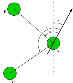
We will use, when possible, the same terms and nota-tions in [17]. In our network each node has one main axis against which all angles are reported and the capacity to estimate the direction from which a neighbor is sending data. We will use the term heading to indicate the angle formed by this main axis with north, represented in Figure 1 by a thick black arrow. The term bearing refers to an angle measurement with respect to another object. In our
B
C
A
h
b c
Figure 1. Node A with its heading and bearings to B and C
case, the AOA capability provides for each node bearings to neighboring nodes with respect to its own axis. In Figure 1, for node A, bearing to B is b, bearing to C is c, and heading is h. When interacting with two neighbors, as shown in Figure 1, a node can find out the angle between its own axis and the direction the signals come from. Node A has the possibility of inferring the angle αBAC
formed by the neighbors B and C as c−b. For the sake of consistency, all angles are assumed to be measured in trigonometric direction.
B. Mathematical bases
The method we propose here is based on the following three steps:
- to define an error functionE measuring the overall relative angle errors of all the nodes in the network; - to apply an optimization method to decrease the error
function;
- to derive a smart distributed algorithm for each node in the networks in such a way that the cooperative behavior implements the optimization method. We assume here that the network consists ofn nodes. Let pi = (xi, yi) be the position of the i-th node in a
two dimensional space. We assume that a node iknows the angle αjik that it forms with each pair of neighbors
j, k. Let Ri be the transmission range of a node i, we
define the set of neighborsN(i)as the set of all the nodes within the transmission rangeRiofi. Note that we do not
assume that the transmission range is the same for each node. As the algorithm has to be completely distributed, we assume that each node estimates its position pi by a
vectorpi= (xi, yi)Then, letαjik be the angle formed by
the estimated positionpiwith the two estimated positions
pj andpj: we call this value estimated angle.
following error function E:
E=X
i
E(pi) =
1 2
X
i
X
j,k∈N(i)
(αjik−αjik)2
This function can be considered a measure of the angle errors sinceEis equal to zero when all the nodes correctly estimate their angles (that is αjik ≡αjik for each iand
for each j, k∈N(i)).
As a second step, we have to chose a method to decrement this function by giving a better estimation of the node angles. The simple gradient descent method is adopted here. This corresponds to performing steepest descent on a surface in estimated angle space whose height at any point of the space is equal at the error measure. As a consequence, we will modify the estimated coordinates of each node iin dependence of E(pi). I.e., we apply a change to pi opposite to the direction
∇E(pi) =
µ ∂E(pi)
∂xi ,
∂E(pi)
∂yi
(1)
.
Then, to determine how to change xi, we have to
evaluate ∆xi = −λ∂E∂x(pii), where λ is a fixed positive
constant. Analogously,∆yi=−λ∂E∂y(pii).
It can be calculated that:
∂E(pi)
∂xi =
X
j,k∈N(i) µ
(αjik−αjik)∂αjik
∂xi +
(2)
+ (αijk−αijk)∂αijk
∂xi + (αikj−αikj)
∂αikj
∂xi
∂E(pi)
∂yi can be calculated accordingly depending on ∂αjik
∂yi ,
∂αijk
∂yi , and
∂αikj
∂yi .
After some mathematic elaboration, and by defining the quantities ux =xi−xj, uy =yi−yj, vx =xi−xk,
vy=yi−yk in order to obtain a compact formulation, it
can be calculated that:
∂αjik
∂xi
=− uy u2
x+u2y
+ vy v2
x+vy2
∂αijk
∂xi
= uy u2
x+u2y
∂αikj
∂xi
=− vy v2
x+v2y
(3)
∂αjik
∂yi
= ux u2
x+u2y
− vx v2
x+v2y
∂αijk
∂yi
=− ux u2
x+u2y
∂αikj
∂yi
= vx v2
x+v2y
. (4)
III. ADISTRIBUTED ALGORITHM
In general, the error functions like E are not convex functions: this is a consequence of NP-completeness of the localization problem based on AOA [20]. Then any exact method to solve this problem will require an expo-nential time for generic instances of the problem (unless
P=NP). Therefore, only approximated solutions can be obtained if a convergence in polinomial time is sought.
Following the method described in the previous section to find a point in the error space with a lower value of the function E, we could implement the sequential (not distributed) Algorithm 1. Then we can repeat the algorithm many times to find lower and lower values of the error function.
Algorithm 1 One step of the sequential algorithm Require: Network topology,pi for each node i Ensure: a new estimation ofpi for each nodei
1: for each nodeido
2: Compute∆xi,∆yi
3: end for
4: for each nodeido
5: xi=xi+ ∆xi,yi=yi+ ∆yi
6: end for
There are two problems to distribute this algorithm: 1) cycles 1- 3 and 4-6 must be computed in two separate phases and this will result in a unacceptable synchroniza-tion among all the nodes in the network to be achieved when the first phase ends. 2) The computation of a single variation at step 2 (e.g.,∆xi) requires that a node knows
the estimated positions and the relative angles of all its neighbors (see Equation 2). In a network with intermittent nodes having no possibility to communicate with more than a neighbor at the same time, this could result in a possible long (may be endless) wait for all the needed data.
We propose to remove both these two constraints by assuming that a node can update its estimated position as soon as it receives new data from a single neighbor node. Telling poorly, a node computes the part of the sum in the Equation (2) relative to its neighbors. Even if this strategy will result in a method that does not follow the negative gradient properly, experimental tests show that there are no significant degradation of results, provided that all the nodes receive data from some of their neighbors within a given interval of time.
In order to compute the sum in Equation (2), each node should receive from a neighbor j its estimated position
pj, together with all angles calculated by j related to each pair of nodes inN(j). It is appropriate (to avoid a
n
2
data transmission size for a node withnneighbors) for a node to send a list Lj of n measured bearings,
leaving to the receiving nodes the calculation task. We defineN(i)˙ as the set of neighbors of nodeifrom which
i has received a signal (obviously N˙(i) ⊆ N(i)). Let
AOAj(k) be the bearing of node k observed by node
j. The list Lj that a node j have to send will be then
composed of the sequence of pairs(k,AOAj(k))for each
k∈N˙(j). Algorithm 2 details the steps performed by a single node i. Node i calculates αjik as the difference
Algorithm 2 Update algorithm for a node i
Require: pj, angle of arrival ofj, and listLj for eachj ∈N(i)˙ Ensure: a new estimation of pi
1: a= 0, b= 0 2: foreachj ∈N(i)˙
3: foreachk∈N˙(i),k6=j
4: calculate αjik,αjik,αijk,αikj, ∂α∂xjiki , ∂α∂xijki , ∂α∂xikji , ∂α∂yjik
i ,
∂αijk
∂yi , ∂αikj
∂yi
5: if (i∈N˙(j)ANDk∈N(j)˙ ) OR (i∈N(k)˙ AND j∈N˙(k)) 6: calculate αijk,αikj
7: a=a+ (αjik−αjik)∂α∂xjiki + (αijk−αijk)∂α∂xijki + (αikj−αikj)∂α∂xikji
8: b=b+ (αjik−αjik)∂α∂yjik
i + (αijk−αijk)
∂αijk
∂yi + (αikj−αikj)
∂αikj
∂yi
9: end if
10: end foreach
11: end foreach
12: xi=xi−λa
13: yi=yi−λb
of estimated angle and equations (3-4)). αijk and αikj
can be computed on the bases of data contained in Lj
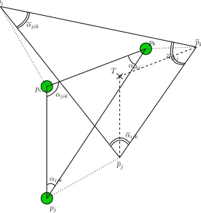
andLk. Let us consider the situation shown in Figure 2
αijk
αjik
pj
αijk
pk
pi
αikj
αjik
pi
pj
T αikj pk
Figure 2. Actual positions and angles among three nodes compared to estimated positions and angles
where nodes i, j, and k are inside the transmission range of each other. pi,pj, andpk indicate the estimated
positions. Dotted lines represent the estimated position errors. After node ihas received signals fromj andk, it is able to calculate αjik. If j, for example, has already
transmitted the bearings ofiandkfrom its point of view (i, k ∈ N(j)˙ ), i is able to calculate αijk. αikj can be
calculated by the same strategy, if i, j∈N(k)˙ , or, as an alternative, it can obtained as 2π−αjik−αijk. At this
point, using the distributed algorithm, nodei can update its estimated positionpiwhich will tend to the target point
T, that is the vertex of the triangle built on the estimated positions pj, andpk with anglesαjik,αijk, andαikj.
Each node, before sending a signal, has to prepare a transmission packet containing its estimated position and the bearing of the signals received from its neighbors. A node receiving such a packet updates the angle of arrival of the sending node in its database and, if possible, updates its estimated position. As a node could receive
more than one packet from the same neighbor, the value of the bearing stored in the database is the mean of all measured values; this will have a positive influence on the algorithm effectiveness, es exposed in Section IV.
Around 180 bytes can be considered a reasonable packet size [23]. Using 32 bit real number to transmit position and angle values and 64 bit integers to transmit node identifiers, a single packet can be sufficient to send all required data for networks with connectivity up to 15 (meaning that each node has up to 15 neighbors). For more dense networks, a simple strategy for rotating data to be sent could be implemented.
A big consequence given by relaxing the constraints of the sequential algorithm is that the resulting distributed algorithm can be used on networks with either stable nodes or nodes with low mobility, just assuming that angle measurements are performed periodically or during the transmission of the estimated positions. Another property of this algorithm is that it is completely asynchronous: a node can start its computation at any time, there is no need for an overall starting criterion, and new nodes can join the network at random times, relative to each other. A characteristic is that there is no explicit terminating con-dition for the overall process: depending on the network is stable or made by mobile sensors, the nodes can stop their computation after a certain number of steps (see next section) or they can perform a round of the Algorithm 2 periodically during their living time. In the next section, we study the behavior of the overall distributed process carried out on stable networks.
IV. EXPERIMENTAL EVALUATION
A. Experimental set-up
In each experiment, a set of nodes, with a certain per-centage of anchors, is placed randomly in a squared area
L×L. For each node a unique value of communication range, set at0.3L, has been considered. The total number of nodes is 100 for each experiment; this value leads to an average connectivity of 10.5 for each node. At the beginning of an experiment each node sets the initial value of its estimated position to a random-chosen point. Every experiment is logically subdived into steps; at each step, a single randomly chosen node “talks”, i.e. it sends a packet containing its estimated position and collected information from neighbor nodes (e.g., the first node to talk will send only its estimated position; the second one will send its estimated position and the bearing of the first node if this is inside its communication range, and so on). At each step, moreover, each node locally applies the Algorithm 2, according to received data. Note that a node has the possibility to update its estimated position only when it has received packets from at least two different neighbors which are in the communication range of each other. A Gaussian noise is added to each bearing to simulate measurement error, as in [17].
B. Results
We graphically report the results obtained by carrying out a first set of experiments in which the initial estimated positions are randomly chosen inside the area. Each ex-periment, characterized by a fixed number of parameters, has been repeated ten times and presented data have to be intended as mean values together with the standard deviation.
Figure 3 shows the position error, represented relative to the communication range, after 10000 steps of the simulation algorithm (the average number of packets sent by a node is therefore 100). On the horizontal axis the standard deviation of the measurement error is varied from 0 to π4, and there is a curve for each different anchor ratio. It can be noticed that for an anchor ratio greater than 10%, the average error is under the 5% of the communication range.
0 0.2 0.4 0.6 0.8 1 1.2 1.4 1.6 1.8
0 π/32 π/16 π/8 π/4
Mean error (# of hops)
Measurement error standard deviation an=5%
an=10%
an=20% an=35%
Figure 3. Positioning error: starting from a completely random initial position, 5% of anchors in not enough to solve the problem
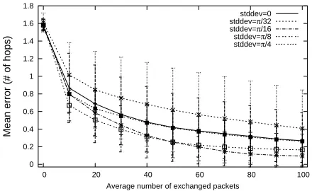
Figures 4 and 5 show the evolution of the location error. In Figure 4 a 10% anchor ratio is considered and there is a
curve for each value of standard deviation of measurement error (0,32π,16π,π8,π4).
0 0.2 0.4 0.6 0.8 1 1.2 1.4 1.6 1.8
0 20 40 60 80 100
Mean error (# of hops)
Average number of exchanged packets stddev=0 stddev=π/32 stddev=π/16 stddev=π/8 stddev=π/4
Figure 4. Positioning error variation for 10% anchor ratio and different measurement error standard deviations
0 0.2 0.4 0.6 0.8 1 1.2 1.4 1.6 1.8
0 20 40 60 80 100
Mean error (# of hops)
Average number of exchanged packets
an=5%
an=10%
an=20% an=35%
Figure 5. Positioning error variation forπ4 measurement error standard deviation and different anchor ratios
It is important to note that the simulation results in Figures 3 and 4 show that Algorithm 2 is robust against measurement error. In fact, results are slightly affected even by big measurement errors: a standard deviation of
π
4 (the highest considered value) implies that the 95% of measurements are in the interval (−π
2,π2)of the true bearing. The fact that each node exploits multiple packets from the same neighbor by considering the mean value of measured bearings instead of a single measurement, significatively contributes to the robustness of Algorithm 2.
In Figure 5, for a standard deviation of π4, there is a curve for each anchor ratio. As expected, a greater anchor ratio positively influences both final result and convergence speed. Even if the algorithm does not treat in a different way informations from the anchors, their right position estimations has a positive influence to the overall convergence.
good position estimation for nodes in the network starting from very unfavorable initial estimated position. For this reason, we carried on a second set of experiments in which we gave a small restriction to the starting position estimation for each nodei, setting it to a random-chosen point inside the square of sideLcentered inpi, instead of
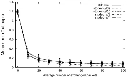
the whole area. Figure 6, 7 and 8 show the results for this kind of experiment. Results have a general considerable enhancement, both in values and in convergence speed. In particular, the curve for 10% anchor ratio has now a behaviour comparable to that obtained with higher anchor ratio in previous experiments (compare Figures 3 and 6).
0 0.05 0.1 0.15 0.2 0.25 0.3 0.35
0 π/32 π/16 π/8 π/4
Mean error (# of hops)
Measurement error standard deviation an=5%
an=10%
an=20% an=35%
Figure 6. Positioning error with finer starting position estimation: the error is quite reduced even for 5% anchor ratio
0 0.2 0.4 0.6 0.8 1 1.2 1.4
0 20 40 60 80 100
Mean error (# of hops)
Average number of exchanged packets stddev=0 stddev=π/32 stddev=π/16 stddev=π/8 stddev=π/4
Figure 7. Positioning error variation for 10% anchor ratio and differ-ent measuremdiffer-ent error standard deviations with finer starting position estimation
In the curve in Figure 6 relative to 5% anchor ratio, there is still a high variance value; this can be explained by the fact that the random placing of a small number of anchors (5 in this case) can be distributed in a not uniform way. To deal with this eventuality, we carried on a further set of experiments in which the small fraction of anchors is homogeneously distributed in the area. In particular we placed them in a circular configuration centered in the L×L square with radium 0.4L. Results for these experiments are reported in Figure 9. The homogeneous placing of anchors results in a reduction in positioning error together with a lower standard deviation, leading to
0 0.2 0.4 0.6 0.8 1 1.2 1.4
0 20 40 60 80 100
Mean error (# of hops)
Average number of exchanged packets
an=5%
an=10% an=20%
an=35%
Figure 8. Positioning error variation for π4 standard deviation mea-surement error and different anchor ratios with finer starting position estimation
performances comparable with those obtained with higher anchor ratio.
0 0.05 0.1 0.15 0.2 0.25 0.3 0.35
0 π/32 π/16 π/8 π/4
Mean error (# of hops)
Measurement error standard deviation
an=5%
Figure 9. Positioning error for 5% anchor ratio with fixed anchor configuration
All the results, even those obtained without restrictions on the initial estimated positions and on the anchor distribution, appear numerically better than those shown in [17] with quite similar simulation assumptions. This consideration, together with the others exposed in the In-troduction, seems to make preferable this new algorithm. A further improvement of the algorithm can be achieved by reducing the number of communications to save power consumption, as explained in next section.
C. Consumption control
For the nature of sensors, even 100 transmitted packets can be considered a significative load. By analyzing the evolution of the error during the execution, it can be seen that after 40-50 exchanged packets, the error reduction can be considered irrelevant. A first step to reduce communication is therefore to limit for each node the number of transmissions to a threshold of 40 packets. As a second step to have a further reduction of consumption, we decided a distributed communication strategy for the nodes, aiming to transmit only useful information.
only applies the Algorithm 2 without sending packets. It will return in ‘transmitting’ state only when it has new information to send. This will happen in the following cases:
- the estimated position of the node is changed of a significative value (0.02L);
- it receives a packet from a new node (therefore having a new bearing to transmit);
- the average value of a bearing is changed of a significative value (0.1 radians).
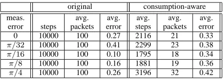
We tested this strategy for an anchor ratio of 10%, the value for which the algorithm has more benefits from the finer initial position estimation. We found that all nodes stop transmitting before reaching the fixed threshold of 40 packets. Tables I and II show the results of such tests, in which experiments have been executed starting from the same initial state of those exposed in the previous section. Each experiment is considered terminated after 100 consecutive steps with all nodes in non-transmitting state. In the tables it is possible to compare the number of steps performed, the average number of packets sent by each node, and the average final position error expressed as a factor of the communication range, obtained by the original version of the algorithm (columns 2, 3, and 4), and by applying the consumption-aware communication strategy (next three columns). Each row of the tables refers to a set of ten experiments characterized by a value of the standard deviation of the measurement error.
TABLE I.
COMPARISON OF ERROR AND NUMBER OF SENT PACKETS IN THE
ALGORITHM WITH AND WITHOUT COMMUNICATION STRATEGY.
original consumption-aware
meas. avg. avg. avg. avg. avg.
error steps packets error steps packets error
0 10000 100 0.27 2116 21 0.33
π/32 10000 100 0.41 2299 23 0.38
π/16 10000 100 0.10 1795 18 0.34
π/8 10000 100 0.16 1881 19 0.36
π/4 10000 100 0.26 3196 32 0.42
Table I, which refer to the totally random initial settings, shows that the average number of transmitted packets largely decreases (compare columns 3 and 6). Moreover, the final average error has a quite limited in-creasement with respect to the original algorithm, keeping the global performance almost unvaried and always better respect to results in [17].
Table II reports the results obtained with the restricted starting position estimation. The final average position error is quite small (between 0.1 and 0.2), but it is larger than that of the original algorithm on the same experiments (less than 0.1). This is not surprising: in fact, further improvements of the estimated positions are not propagated in the network when they are too small to put again nodes in transmitting state.
Comparing columns 6 and 7 of the two tables, it can be noted that consumption-aware algorithm, like the original one, has a benefit in performance with respect both to the
TABLE II.
COMPARISON OF ERROR AND NUMBER OF SENT PACKETS IN THE
ALGORITHM WITH AND WITHOUT COMMUNICATION STRATEGY
WHEN STARTING WITH A FINER INITIAL POSITION ESTIMATION.
original consumption-aware
meas. avg. avg. avg. avg. avg.
error steps packets error steps packets error
0 10000 100 0.069 1569 16 0.203
π/32 10000 100 0.037 1497 15 0.149
π/16 10000 100 0.068 1997 20 0.152
π/8 10000 100 0.076 1831 18 0.153
π/4 10000 100 0.089 2948 29 0.139
number of packets and to the final average position error. Concerning the consumption-aware algorithm, the number of packets for experiments with a measurement error of π/4 is larger with respect all the other exper-iments. This can be explained by the fact that a node remains in transmitting state much longer when a higher measurement error provokes a more frequent update of the mean value of measured bearings. However, a positive consequence of the increased number of packets is that the final estimated positions are almost independent by the measurement error.
V. CONCLUSIONS
A distributed AOA based positioning algorithm has been proposed, it relies on cooperative exchanging of bearing data and estimated location data. From the set of numerical results obtained by a large number of exper-iments, the algorithm can provide satisfactory accuracy, even when energy limitation imposes restrictions to the number of transmitted packets. In particular, an accurate tuning of the parameters used by the consumption-aware version of the distributed algorithm provides good per-formances in terms of limitation of error propagation and reduced load for location and bearing broadcasting.
REFERENCES
[1] “FCC Enhanced 911 - wireless services,” http://www.fcc.gov/911/enhanced/.
[2] D. Niculescu and B. Nath, “Ad hoc positioning system,” in Proceedings of IEEE Globecom, 2001.
[3] N. Bulusu, J. Heidemann, and D. Estrin, “GPS-less low cost outdoor localization for very small devices,” IEEE Personal Communications, Special Issue on Smart Spaces and Environments, vol. 7, no. 5, pp. 28–34, Oct. 2000. [4] L. Doherty, K. S. J. Pister, and L. E. Ghaoui, “Convex
position estimation in wireless sensor networks,” in Pro-ceedings of IEEE INFOCOM, 2001.
[5] T. He, C. Huang, B. M. Blum, J. A. Stankovic, and T. Ab-delzaher, “Range-free localization schemes for large scale sensor networks,” in Proceedings of ACM MOBICOM, 2003.
[6] C. Savarese, J. Rabaey, , and J. Beutel, “Locationing in dis-tributed ad-hoc wireless sensor networks,” in Proceedings of IEEE ICASSP, 2001.
[8] R. Nagpal, H. Shrobe, and J. Bachrach, “Organizing a global coordinate system from local information on an ad hoc sensor network,” in Proceedings of IPSN, 2003. [9] A. Savvides, C. Han, and M. B. Strivastava, “Dynamic
fine-grained localization in ad-hoc networks of sensors,” in Proceedings of ACM MOBICOM, 2001.
[10] A. Savvides, H. Park, and M. B. Srivastava, “The bits and flops of the N-hop multilateration primitive for node localization problems,” in Proceedings of ACM WSNA, 2002.
[11] C. Savarese, J. Rabaey, , and K. Langendoen, “Robust po-sitioning algorithms for distributed ad-hoc wireless sensor networks,” in Proceedings of USENIX Annual Technical Conferenc, 2002.
[12] Y. Shang, W. Ruml, and Y. Zhang, “Localization from mere connectivity,” in Proceedings of ACM MOBIHOC, 2003.
[13] H. Lim and J. C. Hou, “Localization for anisotropic sensor networks,” in Proceedings of ACM INFOCOM, 2005. [14] I. Guvenc, C. T. Abdallah, R. Jordan, and O. Dedeoglu,
“Enhancements to RSS based indoor tracking systems using kalman filters,” in Proceedings of International Sig-nal Processing Conference and Global SigSig-nal Processing Expo, 2003.
[15] D. Niculescu and B. Nath, “Error characteristics of ad hoc positioning systems,” in Proceedings of IEEE MOBIHOC, 2004.
[16] A. S. Krishnakumar and P. Krishnan, “On the accuracy of signal strength-based location estimation techniques,” in Proceedings of ACM INFOCOM, 2005.
[17] D. Niculescu and B. Nath, “Ad hoc positioning system (APS) using AOA,” in Proceedings of IEEE INFOCOM, 2003.
[18] K. Chintalapudi, A. Dhariwal, R. Govindan, and G. Sukhatme, “Ad-Hoc Localization Using Ranging and Sectoring,” in Proceedings of IEEE INFOCOM, 2004. [19] L. Girod, M. Lukac, V. Trifa, and D. Estrin, “The
De-sign and Implementation of a Self-Calibrating Distributed Acoustic Sensing Platform,” in Proceedings of ACM SEN-SYS, 2006.
[20] J. Bruck, J. Gao, and A. Jiang, “Localization and Routing in Sensor Networks by Local Angle Information,” in Proceedings of ACM MOBIHOC, 2005.
[21] G. D. Stefano, F. Graziosi, and F. Santucci, “Distributed positioning algorithm for ad-hoc networks,” in Proceedings of IEEE Int. Workshop on UWB Systems, 2003.
[22] N. B. Priyantha, A. K. Miu, H. Balakrishnan, and S. Teller, “The Cricket compass for context-aware mobile applica-tions,” in Proceedings of IEEE MOBICOM, 2001. [23] Y. Sankarasubramaniam, I. Akyildiz, and
S.W.McLaughlin, “Energy Efficiency Based Packet Size Optimization in Wireless Sensor Networks,” in Proceedings of IEEE SNPA, 2003.
Gabriele Di Stefano obtained his Ph.D. at University ”La Sapienza” of Rome in 1992. Currently he is associate professor for computer science at the University of L’Aquila; his current research interests include network algorithms, combinatorial optimization, algorithmic graph theory; he is (co-)author of more than 50 publications in journals and international conferences. He had key-participations in several EU funded projects. Among them: MILORD (AIM 2024), COLUMBUS (IST 2001-38314), AMORE (HPRN-CT-1999-00104), and, currently, ARRIVAL (IST FP6-021235-2).