Towards Computer-Vision-Based Learning from
Demonstration (CVLfD): Chess Piece Recognition
Regina Wolff
*, Anoshan Indreswaran, Matthias Krauledat, Ronny Hartanto
Rhine-Waal University of Applied Sciences, Faculty of Technology and Bionics, Kleve 47533, Germany.
* Corresponding author. Tel.: +4928218067363628; email: [email protected] Manuscript submitted May 30, 2019; July 12, 2019.
doi: 10.17706/jcp.14.8 519-527.
Abstract: We present an approach to develop algorithms to offer ‘Learning from Demonstration’. Our aim
is to realize Computer Vision as resource-efficient as possible in applications where people interact with computers or -as a special case- with robots. This paper explains the development of a classification program which is to be integrated to a robot that will autonomously play chess. The problem is to perform a classification on a 12 class data set of chess pieces which works on a real-time video feed. We develop two different approaches to solve the problem: A one-step classification is compared to a two-step procedure based on accuracy, computational time and robustness.
Key words: Chess, computer vision, convolutional neuronal network.
1.
Introduction
Computer Vision (CV) is becoming increasingly important in our everyday lives. From leisure activities (3D cinema, Xbox) to device operation (gesture recognition on PC), social media (Facebook facial recognition) to traffic (autonomous cars) – in many areas CV technologies are being tested and used.
Today's standard CV applications are used with machine learning, e.g. in order to detect objects. These are usually trained monitored (supervised). If as many objects as possible are to be detected, large amounts of data (e.g. images) and a high computing capacity are required. Often, supervised and unsupervised approaches are combined [1].
"Learning from Demonstration" is a learning method that is used permanently by us humans: The teacher demonstrates something, the students imitate it. When robots are used, in addition to object recognition, targeted gripping offers an additional challenge: The exact position of objects and optimal gripping surfaces are required. Using CV based "Learning from Demonstration" – algorithms can avoid dangers that can arise from the direct contact of humans and robots in a learning phase. A first approach to this is provided by recent studies of Yezhou [2], which show how individual actions and their combination can be learned and executed by automatic analysis of a video clip by a robot .
The use of this technique is not limited to the use to control a robot: If a computer learns to track objects (tracking) and track operations with the help of a camera, this new ability can be used in many scenarios for communication between humans and computer.
processed by machine learning and an instructions need to be created for the computer/robot. Camera images are thus translated into an abstract description of the process. To do this, detection algorithms need to be expanded accordingly. We call this approach "CV Learning from Demonstration (CVLfD)."
The lessons learned are then used to develop CVLfD – algorithms. At the moment there is a variety of "learning from demonstration – algorithms." The following variants [3], [4] are particularly established: Interactive Reinforcement Learning (Int-RL) , Behavior Networks (BNets), Confidence Based Autonomy (CBA) , and Reinforcement Learning (RL). In our project, different methods are implemented and compared with each other.
Our model project is a chess playing robot [5]. The project is modular, so that the individual modules can also be used independently. Our goal is to develop a chess playing robot which uses camera to visually sense the chess pieces and the surroundings. The objective is to develop object classification architecture with the following key-points:
Minimum computation time, high classification accuracy, the model should be able to learn new objects. In addition, the classification shall be performed from limited number of images that are shot with mobile phone camera.
2.
System Architecture
2.1.
Softwaremodel
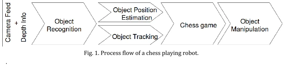
The software development for a chess playing robot can be simplified to the tasks given below:
•Object recognition-: Identifying the different chess pieces, their positions, and the surrounding.
•Object position estimation: Identifying the coordinates of the chess pieces in 3D space of the chess pieces relative to the robot for manipulating the chess pieces.
•Object tracking: Keeping track of the chess moves from the opponent to identify the changes in the game.
•Chess game: The program would include the game methodology and rules for the execution of a well-defined chess game.
Fig. 1. Process flow of a chess playing robot. .
2.2.
Methodologie
There are many factors affecting the performance of a Convolutional Neural Network, such as: the weight initialization, the activation function, the classifier, and the architecture of the network.
Weight initialization is the initial assigning of weights to the neurons. Weights are initialized by assigning constant values, or at random for example, Gaussian weight filler which uses a fixed standard deviation value was introduced. When these techniques were used, the weights were not converging when the number of layers in a network increased.
this project, the weights were initialized using Xavier initialization as it speeds up the training and has a higher probability for convergence.
The activation biases in the fully connected layers were initialized with a constant value of zero. Rectified Linear Units (ReLU) are the better choice compared to the other available functions like sigmoid or hyperbolic tangent, because there is no saturation of weights which would produce dead filters. In addition, the ReLU function is computationally cheap and it converges fast. In the report, we have treated the ReLU layer as a part of the layer on which the activation function is applied, even though whereas defining the architecture the ReLU layers were defined as separate layers. For classification, a Softmax classifier (a feed forward network which uses Softmax loss function) was used in all the models.
This classifier was preferred over the Support Vector Machine (SVM) because of the loss functions nature to always reduce the back propagated loss value. This means, that the output could be interpreted as a confidence level in the classification.
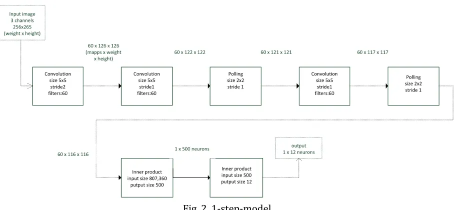
This project presents two architectures for classifying the chess pieces: The 1-Step Model which has a single classifier and the 2-Step Model has two classifiers. The models are explained in the following subsections.
2.3.
1-Step-Model
The 1-Step Model works with HSV images. No prior knowledge is used to breakdown the logic. The input is a HSV image from which features are learned and then used for classification.
The neural network consists of 7 layers excluding the input layer and considering the ReLU layers as a part of the layer (i.e. convolution layer or fully connected layer) which it activates. The first 5 layers are for constructing features and the last two layers are for classifying.
Fig. 2 presents the architecture of the 1-Step Model.
Convolution size 5x5 stride2 filters:60 Convolution size 5x5 stride1 filters:60 Polling size 2x2 stride 1 Convolution size 5x5 stride1 filters:60 Polling size 2x2 stride 1 Inner product input size 807,360
putput size 500
Inner product input size 500 putput size 12 Input image
3 channels 256x265 (weight x height)
60 x 126 x 126 (mapps x weight
x height)
60 x 122 x 122 60 x 121 x 121 60 x 117 x 117
60 x 116 x 116 1 x 500 neurons
output 1 x 12 neurons
Fig. 2. 1-step-model.
2.4.
2-Step-Model
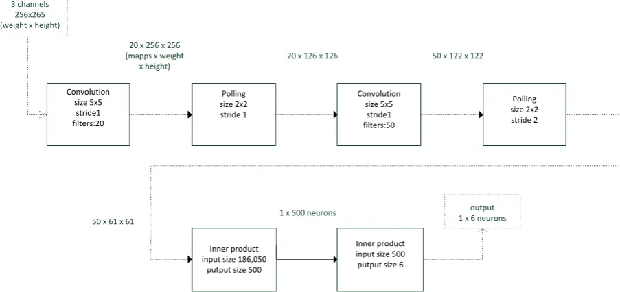
The chess pieces can be grouped into 2 classes based on color, and six different classes based on geometry. Thus we developed a model which uses the Binary classifier to classify the different colors by using the HSV images and the piece-wise classifier on geometry works on the greyscale images.
Convolution size 5x5 stride1 filters:20
Polling size 3 x 3
stride 1
Inner product input size16,820 putput size 200
Inner product input size 200 putput size 2 Input image
3 channels 64 x 65(weight x
height)
20 x 31 x 256 (mapps x weight
x height)
Feature construction Softmax classifier
20 x 29 x 29 1 x 200 neurons
output 1 x 2 neurons
Fig. 3. Architecture of the binary classifier in the 2-step-model.
Fig. 4 depicts the piece-wise classifier's structure. The network has a depth of six layers excluding the input layer and considering the ReLU layers as a part of the layer (i.e. convolution layer or fully connected layer) which it activates. The first 4 layers are the feature constructing layers and the last two layers are for classifying. Convolution size 5x5 stride1 filters:20 Polling size 2x2 stride 1 Convolution size 5x5 stride1 filters:50 Polling size 2x2 stride 2 Inner product input size 186,050
putput size 500
Inner product input size 500 putput size 6 Input image
3 channels 256x265 (weight x height)
20 x 256 x 256 (mapps x weight
x height)
50 x 122 x 122
50 x 61 x 61 1 x 500 neurons
output 1 x 6 neurons 20 x 126 x 126
Fig. 4. Architecture of the shape-based classifier.
3.
Implementation
3.1.
Software
The software used in the program was C++, python and their libraries. The camera was used to capture the necessary video and images for training and testing the network. It was the rear camera of Samsung Note II with 8 MP.
3.2.
Dataset
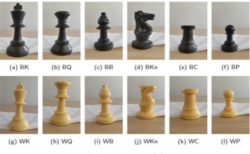
An 8MP rear camera of Samsung Galaxy Note II has been used to take 60 second long videos of frame size1920_1080 pixels of all 12 distinct chess pieces from all around to have different orientations.
Based on this sequences 50 images per class were encoded in JPEG, cropped manually to center the objects, converted to a grayscale and a HSV color space image, resized to 256 x256 pixels and encoded with labels as LMDB. Fig. 2 shows the chess pieces we used to prepare the data set.
Fig. 5. Chess pieces/ data set.
3.3.
Training
The network learns from examples and regulates its learning by losses passed through the network. The learning method, the learning rates, and the required training time are important factor to be considered during training. The stochastic gradient method was chosen for weight updates as it converges fast when used in networks with ReLU activation. The stochastic gradient descent method is a suitable choice if lower training time is necessary.
Since lower learning rate converges slow and the higher learning rate may settle at a local minimum of the loss, the right learning rate for a task is to be found through trial and error [10].
4.
Experiments and Results
Experiments were conducted to study the overall accuracy of the model, the accuracy in classifying individual classes and the computation time. Further analysis was performed to understand the learned features. Further, it provides the results of the experiment to check the robustness of the model to changes in size of the object in the image. The data was split into five subsets from which one subset was used for testing.
The remaining four subsets were used for training. This was done in a repetitive fashion by choosing a new subset from the initial split as the testing set and the remaining as the training until all the subsets were used as a test set. This technique ensures the repeatability of the model for this classification task and its performance as an independent testing set.
The average accuracy of the 1-step model 12 classes is 70%, whereas the overall average accuracy of the 2-step model is 58%. In the 2-step model, the Binary classifier reached 100% accuracy, and the six class classifier processing on gray images reached an average accuracy 58%.her. Table 1 gives the results of the fivefold cross validation performed on both models and the average accuracy.
features for the classes we use a simpler version of the technique used by Zeiler and Fergus [11], [12]. The technique was deployed on the two multi class classifiers and was fed with images of size [300 x 300] pixels for pixel wise classification. The color image classifier classifies using a _filter of size [116 x 116] pixels and the grayscale image classifier uses a filter of size [61 x 61]. The output of the classifier is a matrix of size [23 x 23] with the prediction classes and the confidence of the prediction. This information is used to plot a heatmap to visualize the important regions of a picture during classification.
Table 1. Cross Validation Results
Iteration/ Accuracy
1st 2nd 3rd 4th 5th Average
1-Step classifier
0.7 0.6 0.75 0.75 0.7 0.7
Binary classifier
1.0 1.0 1.0 1.0 1.0 1.0
Piece-wise classifier
0.5 0.8 0.7 0.6 0.3 0.58
2-Step Overall
0.5 0.8 0.7 0.6 0.3 0.58
Fig. 6. Pixel wise classification of a bishop.
The first row contains the input images, the second row the classification heatmaps of the pixel wise classifier.
(a), (b) - HSV image;
(c), (d) - Intensity image displayed as heatmaps
(e), (f) - Classification heatmap of the HSV image (a), (b) respectively (g), (h) - Classification heatmap of the HSV image (c), (d) respectively
region which would result in poor classification performance in situations where the orientation differs or the point of interest is occluded.
Additionally the region of interest in classification of the black bishop is mostly covering the bottom shape and the background of the image. The bottom shape of all the chess pieces is similar which may lead to wrong classification. It is clear the features extracted for learning in the 2-Step model for bishop is bad.
It is clear that the Piece-wise classifier in the 2-Step model needs improvement because the features it has learned are not suitable and too few. The 1-Step model has learned good features, but in the white classes the distribution seems to be too distributed which might be a reason for the poor class wise accuracy in the white pieces.
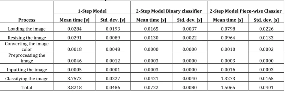
The total classification time is important as the motion of the robot and the chess game algorithm depends on the information it receives from the visual feed. To classify on live video stream without lag, the total time from the capture of video till the output of classification should be less than 500 ms to achieve a prediction with a frame rate of 2 frames per second. Table 2 gives the average time and the standard deviation of the computation. The data was collected from recording the runtime for 60 images.
Table 2. Computation Time of the Different Classifiers
Process
1-Step Model 2-Step Model Binary classifier 2-Step Model Piece-wise Classier Mean time [s] Std. dev. [s] Mean time [s] Std. dev. [s] Mean time [s] Std. dev. [s]
Loading the image 0.0284 0.0193 0.0165 0.0037 0.0798 0.0226
Resizing the image 0.0291 0.0089 0.0130 0.0022 0.0964 0.0133
Converting the image
color 0.0018 0.0048 0.0000 0.0000 0.0010 0.0003
Preprocessing the
image 0.0046 0.0012 0.0003 0.0000 0.0003 0.0000
Inputting the image 0.0005 0.0001 0.0003 0.0000 0.0016 0.0003
Classifying the image 3.7573 0.0227 0.0421 0.0040 1.3273 0.0165
Total 3.8218 0.0486 0.0722 0.0080 1.5065 0.0401
When compared the total time taken for classification, the 2-Step model performs better than the 1-Step model by 2 folds.
5.
Conclusion
This research has been a first step towards our goal to enable machines to “learn from demonstration”
and helps to automatically classify objects in a specific application scenario. Two components of this toolbox have been demonstrated here: the proposed 1-step model with single classifier and the 2-step model with two classifiers. The experiments show that the 1-step model has performed better in most of the aspect compared to the 2-step model. However, it still needs a significant improvement of the algorithm to reduce the classification time such that it becomes usable for real time application. For this purpose, the next step is to verify whether the overall performance of the system run in hardware accelerated systems as well as implementation in different programming languages can improve the speed. Moreover, further experiments will be conducted which includes altered image selection in the learning process in term of number, perspective, exposure, and scales to improve the feature detection.
References
[1] Lenz, I., Lee, H., & Saxena, A. (2015). Deep learning for detecting robotic grasps. The International Journal of
[2] Yezhou, Y. Y. L., Cornelia, F., & Yiannis, A. (2015). Robot learning manipulation action plans by “Watching”
unconstrained videos from the WorldWideWeb. Proceedings of the 29th AAAI Conference on Artificial
Intelligence (Hyatt Regency Austin, January 25, 2015 – January 29, 2015).
[3] Suay, H., Toris, R., & Chernova, S. (2012). A practical comparison of three robot learning from demonstration
algorithm. Int J of Soc Robotics, 4(4), 319-330.
[4] Smart, W. D. Making Reinforcement Learning Work on Real Robots. Brown University, 2002.
[5] Indreswaran, A. (2016). Chess Piece Recognition Using Machine Learning. Rhine-Waal University of Applied
Sciences, 2016.
[6] Glorot, X., & Bengio, Y. (2010). Understanding the difficulty of training deep feedforward neural networks.
City.
[7] Oliphant, T. E. (2006). A Guide to NumPy. Trelgol Publishing USA, 2006. [8] ItseezOpen CV. City.
[9] Kishore, A., Jindal, S., & Singh, S. (2015). Designing Deep Learning Neural Networks Using Caffe.
[10]Karpathy, A. (2016). Cs231n convolutional neural networks for visual recognition. Neural Networks. [11]Zeiler, M. D., & Fergus, R. (2014). Visualizing and Understanding Convolutional Networks. Springer.
[12]Heaton, J. (2015). Artificial intelligence for humans, volume 3: Deep learning and neural networks; heaton
research. Inc.: St. Louis, MO, USA2015, 272-274.
Regina Wolff was born in Kalkar, Germany. She required her University-entrance diploma (Abitur) in 1984, studied informatics at the University Fernuniversität Hagen, Germany and received her computer scientist's diploma (~master) in 1999. In 2010, she became audited IT project coordinator (SGD), Darmstadt, Germany.
She has the following professional experience as a software developer: INPLAN Ruhr, Oberhausen, Germany, IPSEN Int., Kleve, Germany; Kommunales Rechenzentrum Niederrhein KRZN (Municipal Data Center), Kamp-Lindfort, Germany. Since 2011, she works as a research assistant at Rhine-Waal University in the Faculty Technology and Bionics in Kleve, Germany.
Anoshan Indreswaran was been born on Nov 16, 1992 in Sri Lanka. In 2010 -2011, he studied at American National College, Colombo, Sri Lanka.
In 2011 -2018 he studied at Rhine-Waal University in the Faculty Technology and Bionics in Kleve, Germany and received the bachelor mechanical engineering in 2016 and master bionics in 2018.
In 2013, 2014 and 2017 he worked as a student assistant at Rhine-Waal University in the Faculty Technology and Bionics in Kleve, Germany. He had an internship at BMW group and works since 2018 as a project engineer at BMW AG, Munich. His awards include best bachelor in Faculty Technology and Bionics 2016.
RIC Bremen as senior researcher. His research interests are mobile robotics and artificial intelligence with focuses on knowledge representation and reasoning, plan-based robot control, planning algorithms, and machine learning.
Matthias Krauledat studied mathematics at the Westphalian Wilhelms-University Münster, Germany, towards his master’s degree (Dipl. Math.) in 2002. He received his PhD on a thesis titled “Analysis of Nonstationarities in EEG Signals for Improving Brain-Computer Interface Performance” from Technical University Berlin, Germany, in
2008.
As a laboratory head in the central research unit of Henkel AG & Co. KGaA, he applied machine learning methods to industrial production processes. In 2011, he joined the DMT GmbH (TÜV Nord Group) and developed algorithms for condition monitoring of wind turbines. Since 2013, he is a professor for informatics at Rhine-Waal University of Applied Sciences in Kleve, Germany.
Matthias Krauledat’s research interests include applications for the internet of things, big data analysis,