Decomposing international gender test score differences

(1)

ORIGINAL ARTICLE

Decomposing international gender test

score differences

Farzana Munir

1

_{and Rudolf Winter‑Ebmer}

2*

Abstract

In this paper, we decompose worldwide PISA mathematics and reading scores. While mathematics scores are still tilted towards boys, girls have a larger advantage in reading over boys. Girls’ disadvantage in mathematics is increasing over the distribution of talents. Our decomposition shows that part of this increase can be explained by an increasing trend in productive endowments and learning productivity, although the largest part remains unexplained. Countries’ gen‑ eral level of gender (in)equality also contributes to girls’ disadvantage. For reading, at the upper end of the talent distri‑ bution, girls’ advantage can be fully explained by differences in learning productivity, but this is not so at lower levels.

Keywords: Gender gap, Test scores, PISA, Mathematics, Reading

JEL Classification: I23, I24, J16

© The Author(s) 2018. This article is distributed under the terms of the Creative Commons Attribution 4.0 International License (http://creat iveco mmons .org/licen ses/by/4.0/), which permits unrestricted use, distribution, and reproduction in any medium, provided you give appropriate credit to the original author(s) and the source, provide a link to the Creative Commons license, and indicate if changes were made.

1 Introduction

Consensus exists regarding significant gender test score differences in schools. Boys typically excel in mathemat-ics and science whereas girls score better in reading and literacy subjects (e.g., Turner and Bowen 1999; Halpern et al. 2007; Ceci et al. 2009). Although girls have some-what caught up in mathematics (Hyde and Mertz 2009), differences remain. On the other hand, there is evidence of more men or boys at the upper end of the education or professional distribution (Machin and Pekkarinen 2008), which could be attributed to the larger variance of test scores for boys. The magnitude, spread and practi-cal significance of gender differences in educational out-comes have remained a topic of concern. This concern is important, because gender disparities in achievement at an earlier stage, particularly at the upper ends of the distribution, may impact career selection and educational outcomes at a later stage.

The previous literature mostly examined mean differ-ences (Fryer and Levitt 2010), while quantile regressions do exist for some countries (Gevrek and Seiberlich 2014; Sohn 2012; Thu Le and Nguyen 2018): providing evidence for Turkey, Korea and Australia, respectively. Two possible

arguments have been suggested for these gender gaps, one biological or natural (Benbow and Stanley 1980; Geary 1998) and the other environmental, including family, institutional, social, and cultural influences (e.g., Fennema and Sherman 1978; Parsons et al. 1982; Levine and Orn-stein 1983; Guiso et al. 2008; Pope and Sydnor 2010; Nol-lenberger et al. 2016). Recent studies looked at the impact of culture: Nollenberger et al. (2016) look at immigrants in the U.S. to explain whether gender-related culture in the home country can explain differences in mathematics scores; similarly Guiso et al. (2008) look at gender differ-ences in 35 countries PISA mathematics scores.

The present study looks at mathematics and reading scores for all countries included in the OECD’s PISA test and tries to decompose these score differences at different percentiles of the distribution through natural and environmental factors that influence the students’ mathematics and reading test scores. This decomposi-tion research is guided by the Juhn et al. (1993) decom-position model, which extends the usual Blinder–Oaxaca decomposition by taking into account the residual distri-bution. Following this method, this study will decompose test score gaps between males and females to analyze how much of the test score gap can be “predicted” by observable differences across students in determining the test score production function and inequality within these classifications.

Open Access

*Correspondence: [email protected]

2_{Christian Doppler Laboratory Aging, Health and the Labor Market, IZA,} CEPR and IHS, Johannes Kepler University, Linz, Austria

(2)

In this study, we employed international PISA data to examine test score differences between boys and girls worldwide, focusing on the differences at different quan-tiles of the distribution. PISA has the advantage of cover-ing various personal, family, school system, and societal background characteristics, which enables decomposing potential differences into effects due to different endow-ments, institutional settings, and the productivity of learning in different situations. We adopted a decompo-sition following Juhn et al. (1993), which enabled us to decompose test score differentials into endowment, pro-ductivity, and unobservable components.

Our decomposition for score differentials in math-ematics shows that part of the increasing disadvantage of girls over the distribution of talent can be explained by an increasing trend in productive endowments and learning productivity, although the largest part remains unexplained. Countries’ general level of gender (in)equal-ity also contributes to girls’ disadvantage. For reading, at the upper end of the talent distribution, girls’ advantage can be fully explained by differences in learning produc-tivity, but this is not so at lower levels. Our contribution to the literature lies in an extension of quantile regression results to practically all PISA countries, to an inclusion of country-specific gender-related variables and to an appli-cation of the Juhn, Murphy and Pierce analysis, which extends a simple decomposition to take the residual dis-tribution into account.

The remainder of the paper is organized as follows: The next section describes the PISA database, its features and other data sources used in the study. Section 3 discusses the estimation strategy used in this paper and structures the econometric model based upon the Juhn, Murphy

and Pierce decomposition method. Section 4 presents

results on test score inequality for our dispersion analy-sis. Section 5 concludes.

2 Data

This paper uses the micro data of the Program of Interna-tional Student Assessment (PISA) 2012 as well as data on per capita GDP (PPP), gender equality, and government expenditure on education to analyze the decomposition of gender differences in test scores. Combining the avail-able data, the dataset contains information on 480,174 students in 65 countries pertaining to mathematics and reading literacy.

2.1 PISA data

PISA is a cross-national study created by the Organi-zation for Economic Co-operation and Development (OECD) to assess students’ ability in mathematics, read-ing, science, and problem solving. Since its launch in 2000, the assessment is conducted on a triennial basis.

The main advantage of the program is its international comparability, as it assesses students’ ability based on a cohort of students of the same age. Moreover, there is a large volume of background information of students and schools, which may help to put student assessment into perspective. The assessment in each wave focuses on one particular subject,1_{and tests other main areas as well. In} our analysis, we employed data from the 2012 PISA wave that focused on performance in mathematics.

The PISA 2012 dataset covers the test score perfor-mance of students from 34 OECD and 31 non-OECD countries, which includes approximately 510,000 stu-dents aged 15 or 16 years. The dataset includes a number of demographic and socioeconomic variables for these students. The instrument was paper-based and com-prised a mixture of text responses and multiple-choice questions. The test is completed in 2 h. The questions are organized in groups based on real life situations. A strati-fied sampling design was used for this complex survey, and at least 150 schools were selected2_{in each country} and 35 students randomly selected in each school to form clusters. Because of potential sample selection problems, weights were assigned to each student and school. The PISA test scores are standardized with an average score of 500 points and standard deviation of 100 points in OECD countries. In the PISA 2012 test, the final profi-ciency estimates were provided for each student and recorded as a set of five plausible values.3_{In this study,} we used the first plausible value as a measure of student proficiency.4

In 2012, Shanghai scored best and remained at the top with 613 PISA points in mathematics, followed by Hong Kong, Japan, Taiwan, and South Korea, all

1 _{The first PISA exam in 2000 focused on reading literacy, while the second} focused on mathematics specialization. PISA 2012 again focused on math-ematics literacy.

2_{The PISA consortium decides which school will participate, and then the} school provides a list of eligible students. Students are selected by national project managers according to standardized procedures (OECD 2012). 3_{These plausible values are calculated by the complex item-response} the-ory (IRT) model (see Baker 2001; Von Davier and Sinharay 2013) based on the assumption that each student only answers a random subset of ques-tions and their true ability cannot be directly judged but only estimated from their answers to the test. This is a statistical concept, and instead of obtaining a point estimate [like a Weighted Likelihood Estimator (WLE)], a range of possible values of students’ ability with an associated probability for each of these values is estimated (OECD 2009).

4_{“Working with one plausible value instead of five provides unbiased} esti-mates of population parameters but will not estimate the imputation error that reflects the influence of test unreliability for the parameter estimation” (OECD 2009).

(3)

high-performing East Asian countries. Among the Euro-pean countries, Liechtenstein and Switzerland demon-strated the best performance, followed by the Netherlands, Estonia, Finland, Poland, Belgium, Germany, and Austria with slightly lower figures. On average, the mean score in mathematics was 494 and 496 for reading in OECD coun-tries. The UK, Ireland, New Zealand, and Australia were close to the OECD average, while the USA scored lower than the OECD average with 481 PISA points.

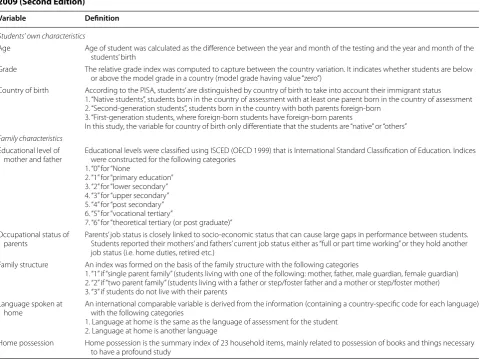
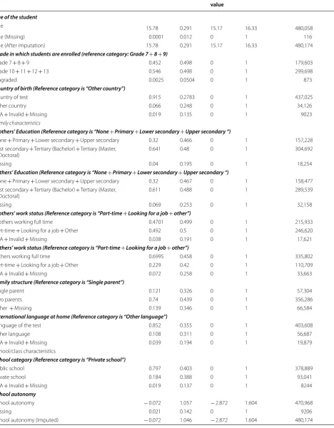
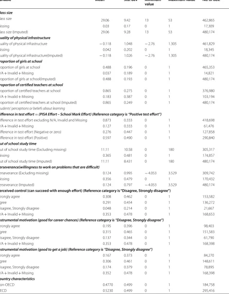
Since the primary concern of this study is to explore the differences in mathematics and reading test scores between male and female students, the dependent vari-able is the student test score in PISA 2012. The rich set of covariates includes five characteristics, namely individual characteristics of the students, their family characteris-tics, school characterischaracteris-tics, student’s beliefs or percep-tions about learning, and country characteristics. Table 2 provides a description of all variables from the PISA data used in this study.

In the survey data, the probability that individuals will be sampled is assumed dependent on the survey design. To take into account this feature, students’ educational production functions were estimated using survey regression methods. This allowed us to include student weights and school clusters depending on the sampling probabilities and within standard errors respectively in our analysis.

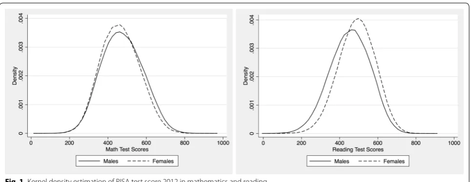
Non-parametric kernel density estimates for the dis-tribution of the entire sample of students’ test score achievements by gender are presented in Fig. 1. The left and right panels of Fig. 1 display kernel density estimates for mathematics and reading test performances respec-tively. Males’ test scores in mathematics are on average higher than those for females, whereas females on aver-age score better than males for reading. Regarding the spread of the curves, it is narrow and highly concentrated

around the mean for females compared to the relatively wider distribution of males both in mathematics and reading test scores.

2.2 Level of development, education expenditure, and gender equality data

To consider the country’s level of development in this analysis, we employed the data on GDP per capita (measured in purchasing power parity (PPP)) from the World Development Indicators 2012. Data on educa-tion expenditure was derived from the Human Devel-opment Report 2013, United Nations DevelDevel-opment Program, while data for Jordan, Shanghai, and Macao were obtained from the World Bank database.

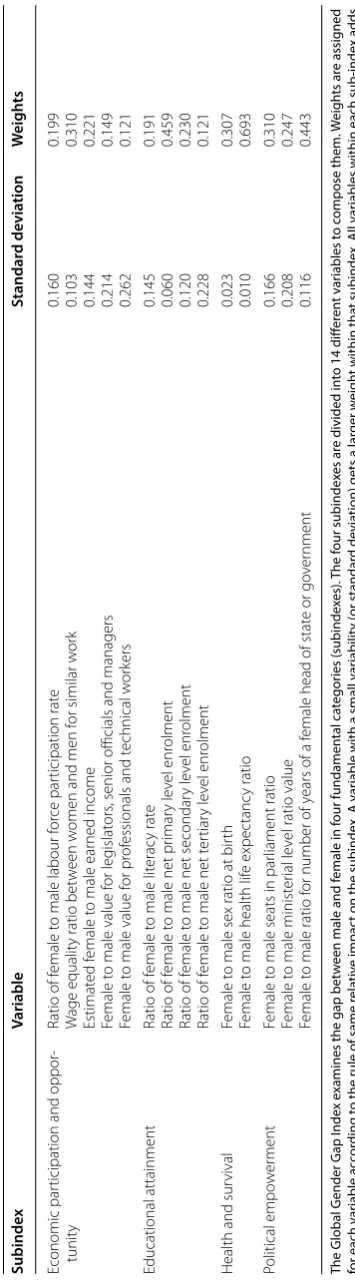
To explore the cultural role related to gender equality, following Guiso et al. (2008), we employed the Gender Gap Index (GGI) by the World Economic Forum (Haus-mann et al. 2013). The Global Gender Gap Index was first introduced in 2006, which by that time was published annually by the World Economic Forum. GGI shows the ranking of countries based on the average of four sub indices,5_{namely economic, political, health, and} edu-cational opportunities provided to females. A GGI of 1 reflects full gender equality and 0 total gender inequality. The top five countries in the 2012 GGI ranking were Ice-land (0.86), FinIce-land (0.85), Norway (0.84), Sweden (0.82), and Ireland (0.78). It is important to note that GGI data is only available for whole countries6_{and not for} partici-pating economic regions in the PISA 2012 dataset (e.g., Hong Kong, Macao, and Shanghai), Furthermore, it does not seem reasonable that data for whole countries can be

Fig. 1 Kernel density estimation of PISA test score 2012 in mathematics and reading

(4)

representative of the relevant economic regions. These regions were eliminated from the data set.7

3 Estimation strategy

In general, decomposition approaches follow the stand-ard partial equilibrium approach in which observed out-comes of one group (i.e., gender, region, or time period) can be used to construct various counterfactual scenarios for the other group. Besides this, decompositions also provide useful indications of particular hypotheses to be explored in more detail (Fortin et al. 2011).

Originally, decomposition methods were proposed by Oaxaca (1973) and Blinder (1973) for decomposing dif-ferences in the means of an outcome variable. The Juhn et al. (JMP) (1993) decomposition method extends the Oaxaca/Blinder decomposition by considering the resid-ual distribution.8_{We show this decomposition following} the description of Sierminska et al. (2010) as follows:

where Yj are the test scores for j=M, W (men and women

respectively), Xj are observables, βj are the vectors of the

estimated coefficients, and εj are the residuals

(unobserv-ables, i.e., unmeasured prices and quantities).

If Fj(.) denotes the cumulative distribution function of

the residuals for group j, then the residual gap consists of two components: an individual’s percentile in the residual distribution pi, and the distribution function of the test

score equation residuals Fj(.). If pij = Fj(εij|xij) is the

per-centile of an individual residual in the residual distribu-tion of model I, by definidistribu-tion we can write the following:

where Fj−1(.) is the inverse of the cumulative distribution

(e.g., the average residual distribution over both samples) and β an estimate of benchmark coefficients (e.g., the coefficients from a pooled model over the whole sample).

Using this framework, we can construct hypothetical outcome distributions with any of the components held fixed. Thus, we can determine:

1. Hypothetical outcomes with varying quantities between the groups and fixed prices (coefficients) and a fixed residual distribution as

(1)

Yj=Xjβj+εj

(2)

εij=F−i 1

p_ij|xij

2. Hypothetical outcomes with varying quantities and varying prices and fixed residual distribution as

3. Outcomes with varying quantities, varying prices,

and a varying residual distribution9_as

Let a capital letter stand for a summary statistic of the distribution of the variable denoted by the correspond-ing lower-case letter. For instance, Y may be the mean or interquartile range of the distribution of y. The differen-tial YM–YW can then be decomposed as follows:

where T is the total difference, Q can be attributed to differences in observable endowments, P to differences in the productivity of observable contributions to test scores, and U to differences in unobservable quantities and prices. This last component not only captures the effects of unmeasured prices and differences in the dis-tribution of unmeasured characteristics (e.g., one of the unmeasured characteristics is more important for men and women for generating test scores), but also measure-ment error.

The major advantage of the JMP framework is that it enables us to examine how differences in the distribution affect other inequality measures and how the effects on inequality differ below and above the mean.

4 Estimation results 4.1 Descriptive statistics

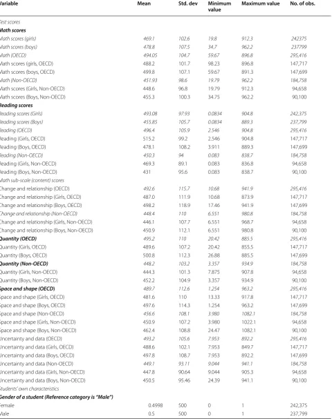
Table 4 contains the descriptive statistics on all the varia-bles used in this microanalysis of the PISA, 2012 dataset. The descriptive statistics are displayed by gender and by OECD and non-OECD countries separately. We imputed missing data for the variable ‘age’ and for some other

(3)

y(_ij1)=xijβ+ F−_i1

p_ij|xij

(4)

y(_ij2)=xijβj+ F−i 1

p_ij|xij

(5)

y(_ij2)= xijβj+F−i 1

p_ij|xij

(6)

YM−YW=

Y(_M1)−Y_W(1)+Y(_M2)−Y(_W2)−Y_M(1)−Y(_W1)

+

Y(_M3)−Y(_W3)−

Y(_M2)−Y(_W2)

=T =Q+P+U

8_{Other methods, like Machado and Mata (}₂₀₀₅_{) provide a similar} decom-position, extending the Blinder-Oaxaca framework along quantiles, Juhn et al. (1993) have the advantage that they also provide for a distribution of residuals.

9 _{These outcomes are actually equal to the originally observed values, i.e.,}

y(_ij3)= yij= xijβj+εij.

(5)

variables10_{in the schooling vector by using the mean} imputation method.

Table 4 shows that in OECD countries, students on

average, scored 42.12 and 46.1 points more in mathe-matics and reading, respectively than non-OECD coun-tries. On average, OECD girls have fallen behind OECD boys by 5.4 points in mathematics scores and 9 points in reading scores, while, non-OECD girls remain 3.5 PISA points behind non-OECD boys in mathematics and 6.5 in reading.

In order to examine whether or not a gender differ-ence within PISA is statistically significant at the 1%, 5% and 10% levels, we also calculated the mean difference between the girls’ and boys’ scores.11_{It shows that} signifi-cant mean differences across gender (based on the OECD and non-OECD grouping) exist for almost all variables.

4.2 PISA score in mathematics

Decomposition results for the mathematical test scores following JMP are depicted in Fig. 2. Positive results indi-cate females’ disadvantage. In Fig. 2, we include a varying set of control variables: individual’s characteristics, fam-ily characteristics, school characteristics, characteristics of beliefs about the learning process, and country char-acteristics. Panels A–E provide the decomposition results including only one of these lists of covariates. Panel F shows a decomposition using all available covariates together. Male–female test score differences are shown at various percentiles: 5th, 10th, 25th, 50th, 75th, 90th, and 95th. Table 6 in Appendix provides the numerical results.

In general, a strong upward trend in the total male– female test score differential (T) is evident. While there is (almost) no difference for the lowest percentiles, the female disadvantage in mathematical competence increases almost linearly to around 20 PISA points at the 95th percentile. As good mathematical knowledge, par-ticularly at the upper percentiles, is especially valuable for getting a good job (Athey et al. 2007), it is important to explore this issue. This total (T) effect will be decom-posed into an effect due to differences in observables (Q), in a productivity-effect (P) on the learning productivity of these observables, and finally, an unobservable (U) rest.

Looking first at Panel F—including all characteristics, this upward trend in mathematical test score differences (T) cannot easily be explained by one factor. Unobserva-bles demonstrate a clear upward trend, but observaUnobserva-bles and productivity effects do so at a somewhat lower level. We now examine individual contributions of individual versus school characteristics. Here, decomposing the

contribution of unobservables (U) in Panels A–E does not make sense, because even if the individual contribu-tions are orthogonal, the unobservable trends measure mainly the impact of omitted variables.

Turning to the contribution of observables (Q) towards mathematical competence, the endowment effect, Panel F indicates a negative endowment effect. In other words, females typically enjoy better endowments: around 10 PISA points at lower percentiles down to 5 PISA points at higher levels. These advantages stem from better female endowments in terms of schooling characteristics and beliefs. The slight upward trend in the contribution of observables in Panel F can mainly be attributed to an upward trend in observables in belief characteristics.

What is the contribution of learning productiv-ity (P)? Panel F shows that the learning productivproductiv-ity of females increases the male–female test score gap for all percentiles, but the effect is slightly higher for higher percentiles. Panels A–E indicate similar productivity dis-advantages for all included lists of characteristics.

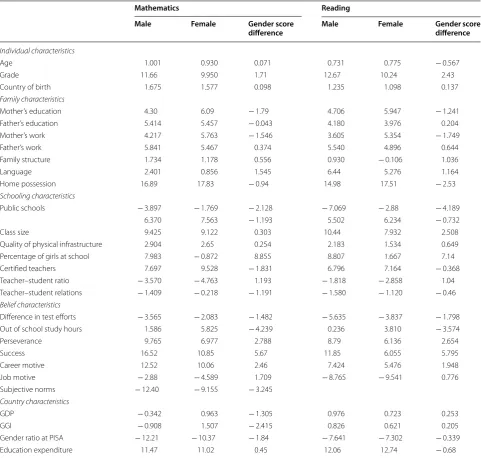
To examine the contribution of individual variables in more detail, we performed the following quantita-tive exercise: increase, in turn, one of the variables in the model by one standard deviation and calculate the impact on the PISA score for males and females (Table 1). Start-ing with variables that will increase the male test score advantage, the number of female students in a classroom has the largest positive effect. Increasing the female share by one standard deviation increases the male–female test score differential by 8.8 PISA points. This is contrary to the results of Gneezy et al. (2003), who found that more female peers in schools increases the mathematical com-petence of females. Other strong pro-male variables are students’ beliefs such as perseverance, success, or a career or job motive. Factors that reduce the male–female gap are subjective norms, public schools, more studying outside school, better education of the mother, and mothers who work more. Interestingly, countries where the GGI is more favorable towards women have lower male–female PISA score differences. This is in contrast to simple correlations by Stoet and Geary (2013), which did not reveal any corre-lation between PISA gender differentials and the GGI.

4.3 PISA scores for reading

An equivalent analysis was conducted for reading, as shown in Fig. 3. Panel F shows the JMP decomposition when all control variables are included. In contrast to mathematics, a continuous advantage of girls over boys is evident. In particular, there is a large disadvantage for boys at the lower end of the distribution: at the 5th and 10th percentile, boys score almost one half standard devi-ation (50 PISA points) less than girls. Torppa et al. (2018) investigate this for an extension of Finnish PISA data 10 _{These are school autonomy, class size, quality of physical infrastructure,}

(6)

and find that general reading fluency (speed) is the main explanation for this difference, whereas other indicators like mastery orientation, homework activity or leisure book reading frequency are not very influential.

On the other hand, similar to mathematics, the total advantage of girls (T) diminishes from around 50 PISA

points at the lowest percentiles to about 20 PISA points at the highest.12_{Decomposing that, at the highest} per-centile levels, this male–female differential is fully

Fig. 2 Juhn–Murphy–Pierce decomposition of relative mathematics test scores by percentile, 2012, T total differential, Q endowments, P

productivity, U unobservables, a–e provide decompositions using only a subset of variables; f uses all available variables

(7)

explained by productivity differentials (P), less so at lower percentiles. There is a contribution of observables (Q): the endowment of students contributes between 6 and 12 PISA points towards this female advantage. Finally, the contribution of unobservables (U) is mixed, increasing between − 9 to + 9 PISA points.

Which factors are responsible for this difference? Our detailed analysis of the causes in Panels A–E in Fig. 3 indicates that endowment differences (Q) are strongest

for schooling characteristics. Schooling characteristics, considered separately, explain between 7 and 10 PISA points, while the contributions of other domains are minor.

On the other hand, there is a large productivity (P) contribution in all separately considered domains. They are particularly high in the family, individual, belief, and country domains.

Table 1 Ceteris–paribus shifts in math and reading test scores due to a one standard deviation shift in individual variables

Gender score inequality is calculated by subtracting the female scores from male scores where positive values are indicating the gender inequality towards females. Male and female test scores are calculated on the basis that one standard deviation increase in particular characteristic e.g. age is associated with an increase of 0.071 score points in math gender score gap

Mathematics Reading

Male Female Gender score

difference Male Female Gender score difference

Individual characteristics

Age 1.001 0.930 0.071 0.731 0.775 − 0.567

Grade 11.66 9.950 1.71 12.67 10.24 2.43

Country of birth 1.675 1.577 0.098 1.235 1.098 0.137

Family characteristics

Mother’s education 4.30 6.09 − 1.79 4.706 5.947 − 1.241

Father’s education 5.414 5.457 − 0.043 4.180 3.976 0.204

Mother’s work 4.217 5.763 − 1.546 3.605 5.354 − 1.749

Father’s work 5.841 5.467 0.374 5.540 4.896 0.644

Family structure 1.734 1.178 0.556 0.930 − 0.106 1.036

Language 2.401 0.856 1.545 6.44 5.276 1.164

Home possession 16.89 17.83 − 0.94 14.98 17.51 − 2.53

Schooling characteristics

Public schools − 3.897 − 1.769 − 2.128 − 7.069 − 2.88 − 4.189

6.370 7.563 − 1.193 5.502 6.234 − 0.732

Class size 9.425 9.122 0.303 10.44 7.932 2.508

Quality of physical infrastructure 2.904 2.65 0.254 2.183 1.534 0.649

Percentage of girls at school 7.983 − 0.872 8.855 8.807 1.667 7.14

Certified teachers 7.697 9.528 − 1.831 6.796 7.164 − 0.368

Teacher–student ratio − 3.570 − 4.763 1.193 − 1.818 − 2.858 1.04

Teacher–student relations − 1.409 − 0.218 − 1.191 − 1.580 − 1.120 − 0.46

Belief characteristics

Difference in test efforts − 3.565 − 2.083 − 1.482 − 5.635 − 3.837 − 1.798

Out of school study hours 1.586 5.825 − 4.239 0.236 3.810 − 3.574

Perseverance 9.765 6.977 2.788 8.79 6.136 2.654

Success 16.52 10.85 5.67 11.85 6.055 5.795

Career motive 12.52 10.06 2.46 7.424 5.476 1.948

Job motive − 2.88 − 4.589 1.709 − 8.765 − 9.541 0.776

Subjective norms − 12.40 − 9.155 − 3.245

Country characteristics

GDP − 0.342 0.963 − 1.305 0.976 0.723 0.253

GGI − 0.908 1.507 − 2.415 0.826 0.621 0.205

Gender ratio at PISA − 12.21 − 10.37 − 1.84 − 7.641 − 7.302 − 0.339

(8)

Regarding the contributions of individual items (Table 1), those favorable for boys are the percentage of girls in a class-room, success motivation, and class size. Factors favorable for girls are public schools and the amount of studying time out of school. Interestingly, a country’s GGI has no effect on the reading differential between boys and girls.

5 Conclusion

In this paper, we provided a decomposition of PISA mathematics and reading scores worldwide. Our contri-bution to the literature lies in an extension of quantile regression results to practically all PISA countries, to an inclusion of country-specific gender-related variables

Fig. 3 Juhn–Murphy–Pierce decomposition of relative reading test scores by percentile, 2012, T total differential, Q endowments, P productivity, U

(9)

and to an application of Juhn et al. (1993) analysis, which extends a simple decomposition to take the residual dis-tribution into account.

While mathematics scores are still tilted towards boys, girls have a larger advantage in reading over boys. This advantage is particularly large for low-achieving indi-viduals. Our analysis shows that over the distribution of talent, boys’ scores increase more than girls—for both mathematics and reading: thus—at the highest percen-tiles—we see a smaller reading advantage for girls as well as a large advantage of boys in mathematics.

Our decomposition shows that part of this increase can be explained by an increasing trend in productive endowments and learning productivity, but the largest part remains unexplained. Countries’ general level of gender (in)equality also contributes towards girls’ dis-advantage. For reading, at the upper end of the talent distribution, girls’ advantage can be fully explained by differences in learning productivity, although this is not so at lower levels. Education policy trying to reduce these gender differences must target high-performing females in their efforts in mathematics and science, and must be

concerned by low-achieving boys who lag in reading and verbal expressiveness.

Authors’ contributions

The authors contributed equally towards the preparation of the paper. Both authors read and approved the final manuscript.

Author details

1_{Bahauddin Zakariya University, Multan, Pakistan.}2_{Christian Doppler Labora‑} tory Aging, Health and the Labor Market, IZA, CEPR and IHS, Johannes Kepler University, Linz, Austria.

Acknowledgements

Thanks to helpful comments to Nicole Schneeweis and Helmut Hofer.

Competing interests

The authors declare that they have no competing interests.

Availability of data materials

Data (PISA) are available for free, Stata‑files are available upon request.

Funding

There is no external funding.

Appendix

See Tables 2, 3, 4, 5, 6, and 7.

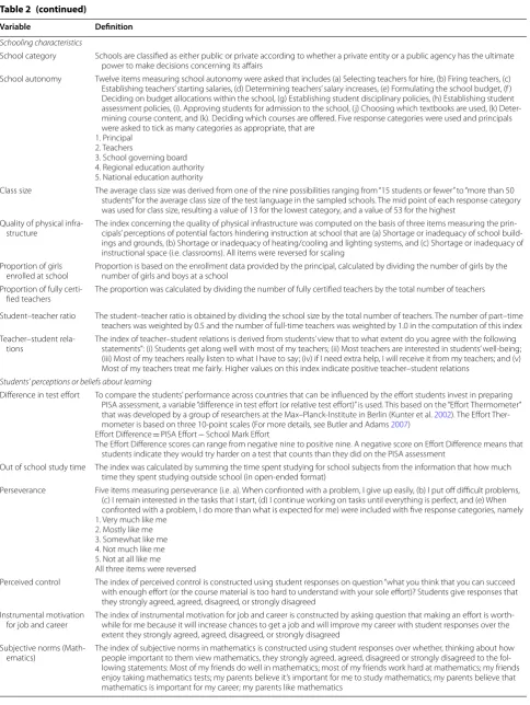
Table 2 Variables’ description (PISA 2012). Sources: (1) PISA Technical Report 2012; (2) PISA Data Analysis Manual SPSS 2009 (Second Edition)

Variable Definition

Students’ own characteristics

Age Age of student was calculated as the difference between the year and month of the testing and the year and month of the

students’ birth

Grade The relative grade index was computed to capture between the country variation. It indicates whether students are below

or above the model grade in a country (model grade having value “zero”)

Country of birth According to the PISA, students’ are distinguished by country of birth to take into account their immigrant status

1. “Native students”, students born in the country of assessment with at least one parent born in the country of assessment 2. “Second‑generation students”, students born in the country with both parents foreign‑born

3. “First‑generation students, where foreign‑born students have foreign‑born parents

In this study, the variable for country of birth only differentiate that the students are “native” or “others” Family characteristics

Educational level of

mother and father Educational levels were classified using ISCED (OECD 1999) that is International Standard Classification of Education. Indices were constructed for the following categories

1. “0” for “None

2. “1” for “primary education” 3. “2” for “lower secondary” 4. “3” for “upper secondary” 5. “4” for “post secondary” 6. “5” for “vocational tertiary”

7. “6” for “theoretical tertiary (or post graduate)” Occupational status of

parents Parents’ job status is closely linked to socio‑economic status that can cause large gaps in performance between students. Students reported their mothers’ and fathers’ current job status either as “full or part time working” or they hold another

job status (i.e. home duties, retired etc.)

Family structure An index was formed on the basis of the family structure with the following categories

1. “1” if “single parent family” (students living with one of the following: mother, father, male guardian, female guardian) 2. “2” if “two parent family” (students living with a father or step/foster father and a mother or step/foster mother) 3. “3” if students do not live with their parents

Language spoken at

home An international comparable variable is derived from the information (containing a country‑specific code for each language) with the following categories

1. Language at home is the same as the language of assessment for the student 2. Language at home is another language

Home possession Home possession is the summary index of 23 household items, mainly related to possession of books and things necessary

(10)

Table 2 (continued)

Variable Definition

School category Schools are classified as either public or private according to whether a private entity or a public agency has the ultimate

power to make decisions concerning its affairs

School autonomy Twelve items measuring school autonomy were asked that includes (a) Selecting teachers for hire, (b) Firing teachers, (c)

Establishing teachers’ starting salaries, (d) Determining teachers’ salary increases, (e) Formulating the school budget, (f ) Deciding on budget allocations within the school, (g) Establishing student disciplinary policies, (h) Establishing student assessment policies, (i). Approving students for admission to the school, (j) Choosing which textbooks are used, (k) Deter‑ mining course content, and (k). Deciding which courses are offered. Five response categories were used and principals were asked to tick as many categories as appropriate, that are

1. Principal 2. Teachers

3. School governing board 4. Regional education authority 5. National education authority

Class size The average class size was derived from one of the nine possibilities ranging from “15 students or fewer” to “more than 50

students” for the average class size of the test language in the sampled schools. The mid point of each response category was used for class size, resulting a value of 13 for the lowest category, and a value of 53 for the highest

Quality of physical infra‑

structure The index concerning the quality of physical infrastructure was computed on the basis of three items measuring the prin‑cipals’ perceptions of potential factors hindering instruction at school that are (a) Shortage or inadequacy of school build‑

ings and grounds, (b) Shortage or inadequacy of heating/cooling and lighting systems, and (c) Shortage or inadequacy of instructional space (i.e. classrooms). All items were reversed for scaling

Proportion of girls

enrolled at school Proportion is based on the enrollment data provided by the principal, calculated by dividing the number of girls by the number of girls and boys at a school

Proportion of fully certi‑

fied teachers The proportion was calculated by dividing the number of fully certified teachers by the total number of teachers

Student–teacher ratio The student–teacher ratio is obtained by dividing the school size by the total number of teachers. The number of part–time

teachers was weighted by 0.5 and the number of full‑time teachers was weighted by 1.0 in the computation of this index Teacher–student rela‑

tions The index of teacher–student relations is derived from students’ view that to what extent do you agree with the following statements”: (i) Students get along well with most of my teachers; (ii) Most teachers are interested in students’ well‑being;

(iii) Most of my teachers really listen to what I have to say; (iv) if I need extra help, I will receive it from my teachers; and (v) Most of my teachers treat me fairly. Higher values on this index indicate positive teacher–student relations

Students’ perceptions or beliefs about learning

Difference in test effort To compare the students’ performance across countries that can be influenced by the effort students invest in preparing

PISA assessment, a variable “difference in test effort (or relative test effort)” is used. This based on the “Effort Thermometer”

that was developed by a group of researchers at the Max–Planck‑Institute in Berlin (Kunter et al. 2002). The Effort Ther‑

mometer is based on three 10‑point scales (For more details, see Butler and Adams 2007)

Effort Difference = PISA Effort − School Mark Effort

The Effort Difference scores can range from negative nine to positive nine. A negative score on Effort Difference means that students indicate they would try harder on a test that counts than they did on the PISA assessment

Out of school study time The index was calculated by summing the time spent studying for school subjects from the information that how much time they spent studying outside school (in open‑ended format)

Perseverance Five items measuring perseverance (i.e. a). When confronted with a problem, I give up easily, (b) I put off difficult problems,

(c) I remain interested in the tasks that I start, (d) I continue working on tasks until everything is perfect, and (e) When confronted with a problem, I do more than what is expected for me) were included with five response categories, namely 1. Very much like me

2. Mostly like me 3. Somewhat like me 4. Not much like me 5. Not at all like me All three items were reversed

Perceived control The index of perceived control is constructed using student responses on question “what you think that you can succeed

with enough effort (or the course material is too hard to understand with your sole effort)? Students give responses that they strongly agreed, agreed, disagreed, or strongly disagreed

Instrumental motivation

for job and career The index of instrumental motivation for job and career is constructed by asking question that making an effort is worth‑while for me because it will increase chances to get a job and will improve my career with student responses over the

extent they strongly agreed, agreed, disagreed, or strongly disagreed Subjective norms (Math‑

ematics) The index of subjective norms in mathematics is constructed using student responses over whether, thinking about how people important to them view mathematics, they strongly agreed, agreed, disagreed or strongly disagreed to the fol‑

(11)

Table 3 S tr uc tur

e of the global gender gap inde

x, 2012. S

our ce: The G lobal G ender G ap Rep or t 2012, W or ld E conomic F or um

The Global G

ender G

ap I

nde

x e

xamines the gap bet

w

een male and f

emale in f

our fundamen tal ca tegor ies (subinde xes). The f our subinde xes ar

e divided in

to 14 diff

er en t v ar iables t o c ompose them. W eigh ts ar e assig ned

for each v

ar

iable ac

cor

ding t

o the rule of same r

ela

tiv

e impac

t on the subinde

x. A v

ar

iable with a small v

ar

iabilit

y (or standar

d devia

tion) gets a lar

ger w

eigh

t within tha

t subinde

x. A

ll v

ar

iables within each sub

‑inde

x adds

to one

. GGI, 2012 is the a

ver

age of the f

our subindic

es

, r

ang

ing fr

om 0 t

o 1 with a max v

alue of 0.86 f

or Ic

eland and minimum v

alue of 0.50 f

or Yemen Subinde x Variable Standar d de via tion W eigh ts Economic par

ticipation and oppor

‑

tunit

y

Ratio of f

emale t

o male labour f

or ce par ticipation rat e W age equalit

y ratio bet

w

een w

omen and men f

or similar w

or

k

Estimat

ed f

emale t

o male ear

ned income

Female t

o male value f

or leg

islat

ors

, senior officials and managers

Female t

o male value f

or pr

of

essionals and t

echnical w

or

kers

0.160 0.103 0.144 0.214 0.262 0.199 0.310 0.221 0.149 0.121

Educational attainment

Ratio of f

emale t

o male lit

erac

y rat

e

Ratio of f

emale t

o male net pr

imar

y le

vel enr

olment

Ratio of f

emale t

o male net secondar

y le

vel enr

olment

Ratio of f

emale t

o male net t

er

tiar

y le

vel enr

olment

0.145 0.060 0.120 0.228 0.191 0.459 0.230 0.121

Health and sur

vival

Female t

o male sex ratio at bir

th

Female t

o male health lif

e expec tanc y ratio 0.023 0.010 0.307 0.693 Political empo w er ment Female t

o male seats in par

liament ratio

Female t

o male minist

er

ial le

vel ratio value

Female t

o male ratio f

or number of y

ears of a f

emale head of stat

e or go

ver

nment

(12)

Table 4 Descriptive statistics

Variable Mean Std. dev Minimum

value Maximum value No. of obs.

Test scores Math scores

Math scores (girls) 469.1 102.6 19.8 912.3 242375

Math scores (boys) 478.8 107.5 34.7 962.2 237799

Math (OECD) 494.05 104.7 59.67 896.8 295,416

Math scores (girls, OECD) 488.2 101.7 98.23 896.8 147,717

Math scores (boys, OECD) 499.8 107.1 59.67 891.3 147,699

Math (Non-OECD) 451.93 98.6 19.79 962.2 184,758

Math scores (Girls, Non‑OECD) 448.6 96.8 19.79 912.3 94,658

Math scores (Boys, Non‑OECD) 455.3 100.3 34.75 962.2 90,100

Reading scores

Reading scores (Girls) 493.08 97.93 0.0834 904.8 242,375

Reading scores (Boys) 455.85 105.7 0.0834 889.3 237,799

Reading (OECD) 496.4 105.9 2.546 904.8 295,416

Reading (Girls, OECD) 515.2 99.2 2.546 904.8 147,717

Reading (Boys, OECD) 478.1 108.2 3.911 889.3 147,699

Reading (Non-OECD) 450.3 94 0.083 838.7 184,758

Reading (Girls, Non‑OECD) 469.3 89.1 0.083 836.8 94,658

Reading (Boys, Non‑OECD) 431 95.6 0.083 838.7 90,100

Math sub-scale (content) scores

Change and relationship (OECD) 492.6 115.7 10.68 941.9 295,416

Change and relationship (Girls, OECD) 487.0 111.9 10.68 873.9 147,717

Change and relationship (Boys, OECD) 498.2 118.9 17.46 941.9 147,699

Change and relationship (Non-OECD) 448.4 110 6.551 980.8 184,758

Change and relationship (Girls, Non‑OECD) 446.1 107.7 6.551 968.7 94,658

Change and relationship (Boys, Non‑OECD) 450.9 112.1 6.551 980.8 90,100

Quantity (OECD) 495.2 110 20.42 885.5 295,416

Quantity (Girls, OECD) 489.6 107.2 20.42 855.5 147,717

Quantity (Boys, OECD) 500.8 112.3 26.88 885.5 147,699

Quantity (Non-OECD) 448.2 103.2 3.357 934.9 184,758

Quantity (Girls, Non‑OECD) 444.3 101.3 7.875 907.8 94,658

Quantity (Boys, Non‑OECD) 452.2 104.9 3.357 934.9 90,100

Space andshape (OECD) 489.7 112.6 1.254 963.2 295,416

Space and shape (Girls, OECD) 481.6 110 13.33 917.8 147,717

Space and shape (Boys, OECD) 497.6 114.3 1.254 963.2 147,699

Space and shape (Non‑OECD) 456.6 108.1 3.980 1082.1 184,758

Space and shape (Girls, Non‑OECD) 450.9 107.2 3.980 1022.1 94,658

Space and shape (Boys, Non‑OECD) 462.4 108.8 24.47 1082.1 90,100

Uncertainty and data (OECD) 493.2 105.6 7.953 892.2 295,416

Uncertainty and data (Girls, OECD) 488.6 102.1 7.953 849.7 147,717

Uncertainty and data (Boys, OECD) 497.8 108.7 7.953 892.2 147,699

Uncertainty and data (Non‑OECD) 449.1 93.11 9.044 941.1 184,758

Uncertainty and data (Girls, Non‑OECD) 447.8 90.64 9.044 905.3 94,658

Uncertainty and data (Boys, Non‑OECD) 450.5 95.46 24.39 941.1 90,100

Students’ own characteristics

Gender of a student (Reference category is “Male”)

Female 0.4998 500 0 1 242,375

(13)

Age of the student

Age _15.78 _0.291 _15.17 _16.33 _480,058

Age (Missing) 0.0001 0.012 0 1 116

Age (After imputation) 15.78 0.291 15.17 16.33 480,174

Grade in which students are enrolled (reference category: Grade 7 + 8 + 9)

Grade 7 + 8 + 9 0.452 0.498 0 1 179,603

Grade 10 + 11 + 12 + 13 0.546 0.498 0 1 299,698

Ungraded 0.0025 0.0504 0 1 873

Country of birth (Reference category is “Other country”)

Country of test 0.915 0.2783 0 1 437,025

Other country 0.066 0.248 0 1 34,126

N/A + Invalid + Missing 0.019 0.135 0 1 9023

Mothers’ Education (Reference category is “None+Primary+Lower secondary+Upper secondary “)

None + Primary + Lower secondary + Upper secondary 0.32 0.466 0 1 157,228

Post secondary + Tertiary (Bachelor) + Tertiary (Master,

Doctoral) 0.641 0.48 0 1 304,692

Missing 0.04 0.195 0 1 18,254

Fathers’ Education (Reference category is “None+Primary+Lower secondary+Upper secondary “)

None + Primary + Lower secondary + Upper secondary 0.32 0.467 0 1 158,477

Post secondary + Tertiary (Bachelor) + Tertiary (Master,

Doctoral) 0.611 0.488 0 1 289,539

Missing 0.069 0.253 0 1 32,158

Mothers’ work status (Reference category is “Part-time+Looking for a job+other”)

Mothers working full time 0.4701 0.499 0 1 215,933

Part‑time + Looking for a job + Other 0.492 0.5 0 1 246,620

N/A + Invalid + Missing 0.038 0.191 0 1 17,621

Fathers’ work status (Reference category is “Part-time+Looking for a job+other”)

Fathers working full time 0.6995 0.458 0 1 335,802

Part‑time + Looking for a job + Other 0.229 0.42 0 1 110,709

Family structure (Reference category is “Single parent”)

Single parent 0.121 0.326 0 1 57,304

Two parents 0.74 0.439 0 1 356,286

Other + Missing 0.139 0.346 0 1 66,584

International language at home (Reference category is “Other language”)

Language of the test 0.852 0.355 0 1 403,608

Other language 0.108 0.311 0 1 56,687

School/class characteristics

School category (Reference category is “Private school”)

Public school 0.797 0.403 0 1 378,889

Private school 0.184 0.388 0 1 93,041

N/A + Invalid + Missing 0.019 0.137 0 1 8244

School autonomy

School autonomy − 0.072 1.057 − 2.872 1.604 470,968

Missing 0.021 0.142 0 1 9206

(14)

Class size

Class size _29.06 _9.42 ₁₃ ₅₃ _462,865

Missing 0.03 0.17 0 1 17,309

Class size (Imputed) 29.06 9.28 13 53 480,174

Quality of physical infrastructure

Quality of physical infrastructure − 0.118 1.048 − 2.76 1.305 461,829

Missing 0.042 0.202 0 1 18,345

Quality of physical infrastructure(Imputed) − 0.118 1.026 − 2.76 1.305 480,174

Proportion of girls at school

Proportion of girls at school 0.488 0.196 0 1 465,353

Proportion of girls at school(Imputed) 0.488 0.193 0 1 480,174

Proportion of certified teachers at school

Proportion of certified teachers at school 0.865 0.275 0 1 376,980

Proportion of certified teachers at school (Imputed) 0.865 0.249 0 1 480,174

Students’ perceptions or beliefs about learning

Difference in test effort = (PISA Effort – School Mark Effort) (Reference category is “Positive test effort”)

Difference in test effort excluding N/A, Invalid and Missing 0.873 0.333 0 1 418,698

Difference in test effort (Negative or zero) 0.276 0.447 0 1 127,858

Difference in test effort (Positive) 0.597 0.490 0 1 290,840

Out of school study time

Out of school study time (Excluding missing) 11.11 10.58 0 180 305,317

Missing 0.365 0.481 0 1 174,857

Out of school study time (Imputed) 11.11 8.431 0 180 480,174

Perseverance(willingness to work on problems that are difficult)

Perseverance (Excluding missing) 0.124 0.995 − 4.053 3.529 309,742

Missing 0.356 0.479 0 1 170,432

Perseverance (Imputed) 0.124 0.797 − 4.053 3.529 480,174

Perceived control (can succeed with enough effort) (Reference category is “Disagree, Strongly disagree”)

Strongly agree 0.308 0.462 0 1 153,582

Agree 0.291 0.454 0 1 136,272

Disagree, Strongly disagree 0.048 0.214 0 1 21,667

Instrumental motivation (good for career chances) (Reference category is “Disagree, Strongly disagree”)

Strongly agree 0.195 0.396 0 1 98,403

Agree 0.315 0.465 0 1 151,583

Instrumental motivation (good to get a job) (Reference category is “Disagree, Strongly disagree”)

Strongly agree 0.167 0.373 0 1 84,270

Agree 0.306 0.461 0 1 148,611

Country characteristics

Non‑OECD 0.4770 0.499 0 1 184,758

(15)

GDP per capita (PPP) 33,937.2 24,246.2 5000.8 135,421.7 479,881

GGI 0.7108 0.0544 0.6015 0.864 452,918

Gender ratio at PISA test 1.019 0.0854 0.84 1.3 478,413

Expenditures on education (%) 5.0116 1.372 2.1 8.7 450,865

Table 5 International gender gap in math and reading test scores at various percentiles

Firstly, we calculated the performance percentiles for girls and boys separately for each assessment and then for each assessment, we calculated the gender differences in performance distribution by subtracting the boys’ scores from girls’ scores

1st 5th 10th 25th 50th = median Std. dev. 75th 90th 95th 99th

Test score performance in mathematics

Girls’ scores 248.8 305.51 336.66 391.97 460.59 100.17 532.96 596.60 632.74 698.17

Boys’scores 246.31 307.14 339.78 398.75 472.12 106.16 549.39 616.30 652.99 717.64

Gender gap = (Girls–Boys) 2.49 − 1.63 − 3.12 − 6.78 − 11.53 − 16.43 − 19.7 − 20.25 − 19.47

Test score performance in reading

Girls’ scores 257.36 327.42 363.88 424.48 491.84 96.49 556.97 612.02 643.32 698.28

Boys’scores 201.99 276.09 315.95 381.95 456.29 105.22 528.46 587.81 620.13 678.35

Gender gap = (Girls–Boys) 55.37 51.33 47.93 42.53 35.55 28.51 24.21 23.19 19.93

Table 6 Juhn–Murphy–Pierce decomposition of mathematics test scores by gender

Percentiles T Q P U

p5 0.6232 − 1.6601 10.627 − 8.3435

p10 1.7136 − 2.6240 11.1438 − 6.8062

p25 4.7516 − 3.0524 11.534 − 3.7298

p50 9.2694 − 2.7514 11.829 0.1914

p75 14.644 − 1.8629 12.234 4.2733

p90 17.916 − 1.4133 12.525 6.8035

p95 18.928 − 1.3949 13.001 7.3219

p5 0.6232 0.3782 9.3689 − 9.1239

p10 1.7136 − 0.8306 9.6578 − 7.1136

p25 4.7516 − 1.2217 9.9602 − 3.9869

p50 9.2694 − 0.3162 9.6565 − 0.0709

p75 14.644 0.9631 9.5052 4.1756

p90 17.916 0.4696 9.8460 7.6000

p95 18.928 0.0490 9.7870 9.0921

p5 0.6232 − 5.9810 15.933 − 9.3289

p10 1.7136 − 7.2584 16.637 − 7.6655

p25 4.7516 − 7.8643 17.044 − 4.4281

p50 9.2694 − 7.6651 16.846 0. .0887

p75 14.644 − 7.4658 17.388 4.7218

p90 17.916 − 7.7754 17.839 7.8517

p95 18.928 − 8.8790 19.016 8.7914

p5 0.6232 − 3.4441 8.5159 − 4.4486

p10 1.7136 − 4.1805 10.000 − 4.1060

p25 4.7516 − 4.1604 11.559 − 2.6474

p50 9.2694 − 2.4598 12.256 − 0.5264

p75 14.644 − 1.5339 13.877 2.3006

p90 17.916 − 1.3770 14.394 4.8983

p95 18.928 − 2.1631 15.337 5.7538

p5 0.0779 2.2793 6.9492 − 9.1506

p10 1.1684 1.2424 7.5482 − 7.6222

p25 4.3621 1.1179 7.8306 − 4.5864

p50 8.2568 0.8006 7.8884 − 0.4322

p75 14.021 1.5481 7.8875 4.5853

p90 17.215 0.95,581 7.8215 8.4372

p95 18.227 0.6335 7.6553 9.9383

All characteristics

p5 0.0779 − 10.119 14.258 − 4.0610

p10 1.1684 − 11.203 15.762 − 3.3903

p25 4.3621 − 10.737 17.339 − 2.2400

p50 8.2568 − 8.1646 16.836 − 0.4148

p75 14.021 − 6.0930 18.046 2.0675

p90 17.215 − 5.4332 18.752 3.8954

p95 18.227 − 6.4822 19.588 5.1214

(16)

Publisher’s Note

Springer Nature remains neutral with regard to jurisdictional claims in pub‑ lished maps and institutional affiliations.

Received: 7 May 2018 Accepted: 30 October 2018

References

Adams, R., Butler, J.: The impact of differential investment of student effort on the outcomes of international studies. J. Appl. Measur. 8(3), 279–304 (2007)

Athey, S., Katz, L.F., Krueger, A.B., Levitt, S.: What does performance in graduate school predict? Graduate economics education and student outcomes. Am. Econ. Rev. Papers Proc. 97(2), 512–520 (2007)

Baker, F. B. (2001). The basics of item response theory. For full text: http://erica e.net/irt/baker

Benbow, C.P., Stanley, J.C.: Sex differences in mathematical ability: fact or artifact? Science 210(4475), 1262–1264 (1980)

Blinder, A.S.: Wage discrimination: reduced form and structural estimates. J. Hum. Resour. 8, 436–455 (1973)

Ceci, S.J., Williams, W.M., Barnett, S.M.: Women’s underrepresentation in science: sociocultural and biological considerations. Psychol. Bull. 135(2), 218 (2009)

Fennema, E.H., Sherman, J.A.: Sex‑related differences in mathematics achieve‑ ment and related factors: a further study. J. Res. Math. Educ. 9, 189–203 (1978)

Fortin, N., Lemieux, T., Firpo, S.: Decomposition methods in economics. Hand‑ book Labor Econ. 4, 1–102 (2011)

Fryer, R.G., Levitt, S.D.: An empirical analysis of the gender gap in mathematics. Ame. Econ. J. 2(2), 210–240 (2010)

Geary, D.C.: Male, female: the evolution of human sex differences. American Psychological Association, London (1998)

Gevrek, Z., Seiberlich, R.: Semiparametric decomposition of the Gender Achievement Gap: an application for Turkey. Labour Econ. 31, 27–44 (2014)

Gneezy, U., Niederle, M., Rustichini, A.: Performance in competitive environ‑ ments: gender differences. Quart. J. Econ. 118(3), 1049–1074 (2003) Guiso, L., Monte, F., Sapienza, P., Zingales, L.: Culture, math, and gender. Science

320(5880), 1164–1165 (2008)

Halpern, D.F., Benbow, C.P., Geary, D.C., Gur, R.C., Hyde, J.S., Gernsbacher, M.A.: The science of sex differences in science and mathematics. Psychol. Sci. Public Interest 8(1), 1–51 (2007)

Hausmann, R., Tyson, L.D., Bekhouche, Y., Zahidi, S.: The global gender gap index 2012. In: World Economic Forum (2013)

Hyde, J.S., Mertz, J.E.: Gender, culture, and mathematics performance. Proc. Natl. Acad. Sci. 106(22), 8801–8807 (2009)

Juhn, C., Murphy, K.M., Pierce, B.: Wage inequality and the rise in returns to skill. J. Polit. Econ. 101(3), 410–442 (1993)

Kunter, M., Gundel Schümer, G., Artelt, C., Baumert, J., Klieme, E., Neubrand, M., Prenzel, M., Schiefele, U., Schneider, W., Stanat, P., Tillmann, K.‑J., Weiß, M.: PISA 2000: dokumentation der erhebungsinstrumente. Materialien aus der Bildungsforschung, Max‑Planck‑Institut für Bildungsforschung (2002) Levine, D.U., Ornstein, A.C.: Sex differences in ability and achievement. J. Res.

Develop. Educ. 16(2), 66–72 (1983)

Machin, S., Pekkarinen, T.: Global Sex Differences in Test Score Variability. Sci‑ ence 322, 1331–1332 (2008)

Machado, J., Mata, J.: Counterfactual decomposition of changes in wage distri‑ butions using quantile regressions. J. Appl. Econ. 20, 445–465 (2005) Munir, F.: Essays on Labor Market Institutions, Growth and Gender Inequality

(Doctoral dissertation). (2017). http://epub.jku.at/obvul ihs/conte nt/title info/18730 92?lang=en

Nollenberger, N., Rodríguez‑Planas, N., Sevilla, A.: The math gender gap: the role of culture. Am. Econ. Rev. 106(5), 257–261 (2016)

Oaxaca, R.: Male–female wage differentials in urban labor markets. Int. Econ. Rev. 14, 693–709 (1973)

OECD.: PISA Data Analysis Manual (Second edition): SPSS. OECD. (2009). http:// www.oecd‑ilibr ary.org/educa tion/pisa_19963 777;jsess ionid =4gvjp s237h iqq.x‑oecd‑live‑02

Table 7 Juhn–Murphy–Pierce decomposition of reading test scores by gender

p5 − 51.798 − 1.9803 − 36.400 − 13.419

p10 − 49.510 − 2.8214 − 35.864 − 10.825

p25 − 44.506 − 3.4393 − 35.142 − 5.9239

p50 − 37.592 − 3.0823 − 34.603 0.0927

p75 − 30.392 − 2.1495 − 34.424 6.1816

p90 − 25.133 − 1.2906 − 33.860 10.018

p95 − 23.075 − 1.4792 − 33.746 12.150

p5 − 51.798 0..6290 − 37.766 − 14.662

p10 − 49.510 − 0.8843 − 36.781 − 11.845

p25 − 44.506 − 1.9307 − 36.540 − 6.0346

p50 − 37.592 − 0.8760 − 36.929 0.2126

p75 − 30.392 0.5776 − 37.222 6.2526

p90 − 25.133 1.4306 − 37.325 10.762

p95 − 23.075 0.9785 − 37.339 13.286

p5 − 51.798 − 6.9977 − 31.159 − 13.642

p10 − 49.510 − 7.9886 − 29.939 − 11.583

p25 − 44.506 − 9.2939 − 28.970 − 6.2421

p50 − 37.592 − 9.0559 − 28.759 0..2229

p75 − 30.392 − 8.3132 − 28.208 6.1292

p90 − 25.133 − 8.4905 − 27.146 10.503

p95 − 23.075 − 10.373 − 25.693 12.992

p5 − 51.798 − 4.7127 − 37.495 − 9.5907

p10 − 49.510 − 4.2156 − 36.305 − 8.9900

p25 − 44.506 − 3.5509 − 34.893 − 6.0617

p50 − 37.592 − 2.1595 − 34.672 − 0.7610

p75 − 30.392 − 1.6176 − 33.969 5.1950

p90 − 25.133 − 1.7336 − 33.013 9.6143

p95 − 23.075 − 2.4504 − 32.282 11.657

p5 − 51.648 1.8113 − 38.138 − 15.321

p10 − 48.883 1.0150 − 37.919 − 11.979

p25 − 44.276 0.6254 − 38.238 − 6.6628

p50 − 38.243 0.4795 − 38.578 − 0.1441

p75 − 30.563 1.3517 − 39.038 7.1231

p90 − 25.540 1.5354 − 39.435 12.360

p95 − 23.638 0.6097 − 39.488 15.240

All characteristics

p5 − 51.648 − 11.752 − 31.189 − 8.7071

p10 − 48.883 − 12.374 − 29.587 − 6.9220

p25 − 44.276 − 12.192 − 28.067 − 4.0162

p50 − 38.243 − 9.9101 − 27.790 − 0.54,317

p75 − 30.563 − 7.1428 − 27.426 4.0055

p90 − 25.540 − 6.4802 − 26.577 7.5171

(17)

OECD.: Bildung auf einen Blick 2012: OECD‑Indikatoren (2012)

Pope, D.G., Sydnor, J.R.: Geographic variation in the gender differences in test scores. J. Econ. Perspect. 24(2), 95–108 (2010)

Parsons, J.E., Meece, J.L., Adler, T.F., Kaczala, C.M.: Sex differences in attributions and learned helplessness. Sex Roles 8(4), 421–432 (1982)

Sierminska, E., Frick, J., Grabka, M.: Examining the gender wealth gap. Oxford Economic Papers 62, 669–690 (2010)

Sohn, K.: A new insight into the gender gap in math. Bull. Econ. Res. 64(1), 135–155 (2012)

Stoet, G., Geary, D.C.: Sex differences in mathematics and reading achievement are inversely related within‑ and across‑nation assessment of 10 years of PISA data. PLoS ONE 8, e57988 (2013)

Thu Le, H., Nguyen, H.T.: The evolution of the gender test score gap through seventh grade: new insights from Australia using unconditional quantile regression and decomposition. IZA J. Labor Econ. (2018). https ://doi. org/10.1186/s4017 2‑018‑0062‑y

Torppa, M., Eklund, K., Sulkunen, S., Niemi, P., Ahonen, T.: Why do boys and girls perform differently on PISA Reading in Finland? The effects of reading fluency, achievement behavior, leisure reading and homework activity. J. Res. Read. 41(1), 122–139 (2018)

Turner, S.E., Bowen, W.G.: Choice of major: the changing (unchanging) gender gap. Ind. Labor Relat. Rev. 52(2), 289–313 (1999)