R E S E A R C H
Open Access
A deep learning framework for
predicting cyber attacks rates
Xing Fang
1*, Maochao Xu
2, Shouhuai Xu
3and Peng Zhao
4Abstract
Like how useful weather forecasting is, the capability of forecasting or predicting cyber threats can never be overestimated. Previous investigations show that cyber attack data exhibits interesting phenomena, such as long-range dependence and high nonlinearity, which impose a particular challenge on modeling and predicting cyber attack rates. Deviating from the statistical approach that is utilized in the literature, in this paper we develop a deep learning framework by utilizing the bi-directional recurrent neural networks with long short-term memory, dubbed BRNN-LSTM. Empirical study shows that BRNN-LSTM achieves a significantly higher prediction accuracy when compared with the statistical approach.
Keywords: ARIMA, GARCH, RNN, Hybrid models, LSTM, Deep learning, BRNN-LSTM
1 Introduction
Cyber attacks have become a prevalent and severe threat against the society, including its infrastructures, econ-omy, and citizens’ privacy. According to a 2017 report by Symantec1, cyber attacks in year 2016 include multi-million dollar virtual bank heists as well as overt attempts to disrupt the U.S. election process; according to another 2017 report by NetDiligence2, the average cyber breach cost is $394K and companies with revenues greater than $2B suffer an average breach cost of $3.2M.
Given the severe consequence of cyber attacks, cyber defense capability needs to be substantially improved. One approach to improving cyber defense is to forecast or pre-dict cyber attacks, similar to how weather forecasting has benefited the society in mitigating natural hazards. The prediction capability can guide defenders to achieve cost-effective, if not optimally, allocation of defense resources [1–4]. For example, the defender may need to allocate more resources for deep packet inspection [5] to accom-modate the predicted high cyber attack rate. Moreover, researchers have studied how to use a Bayesian method to predict the increase or decrease of cyber attacks [6], how to use a hidden Markov model to predict the increase or decrease of Bot agents [7], how to use a seasonal ARIMA
*Correspondence:[email protected]
1School of Information Technology, Illinois State University, Normal 61761, IL, USA
Full list of author information is available at the end of the article
model to predict cyber attacks [8], how to use a FARIMA model to predict cyber attack rates when the time series data exhibits long-range dependence [1], how to use a FARIMA+GARCH model to achieve even more accurate predictions by further accommodating the extreme val-ues exhibited by the time series data [9], how to use a marked point process to model extreme cyber attack rates while considering both magnitudes and inter-arrival times of time series [10], how to use a vine copula model to quantify the effectiveness of cyber defense early-warning mechanisms [11], and how to use a vine copula model to predict multivariate time series of cybersecurity attacks while accommodating the high-dimensional dependence between the time series [12]. We refer to two recent sur-veys on the use of statistical methods in cyber incident and attack detection and prediction [13,14].
A particular kind of cyber threat data is the time series of cyber attacks observed by a cyber defense instru-ment known as honeypots, which passively monitor the incoming Internet connections. Such datasets exhibit rich phenomena, including long-range dependence (LRD) and highly nonlinearity [1,9].
It is worth mentioning that the usefulness of predic-tion capabilities in the context of cyber defense ultimately depends on the degree of prediction accuracy, a situ-ation similar to the usefulness of weather forecasting. This factor should be made fully aware to cyber defense practitioners. Although the prediction accuracy could be
assured by leveraging large amounts of data, which is indeed true to the case of weather forecasting, the col-lection of large amounts of cyber attack data may be challenging. Nevertheless, understanding the usefulness of prediction capabilities in the context of cyber security is a problem of high importance but has yet to be thoroughly investigated.
1.1 Our contributions
The contribution of the present paper is in two-fold. First, we propose a novel bi-directional recurrent neu-ral networks with long short-term memory framework, or BRNN-LSTM for short, to accommodate the statisti-cal properties exhibited by cyber attack rate time series data. The framework gives users the flexibility in choosing the number of LSTM layers that are incorporated into the BRNN structure. Second, we use real-world cyber attack rate datasets to show that BRNN-LSTM can achieve a substantially higher prediction accuracy than statistical prediction models, including the one proposed in litera-ture [9] and the ones that are studied in the present paper for comparison purposes.
1.2 Related work
Statistical methods have been widely used in the context of data-driven cyber security research, such as intru-sion detection [15–18]. However, deep learning has not received the due amount of attention in the context of cyber security [13, 14]. This is true despite the fact that deep learning has been tremendous successful in other application domains [19–21] and has started to be employed in the cyber security domains, including adversarial malware detection [22, 23] and vulnerability detection [24,25].
In the context of vulnerability detection, supervised machine learning methods inlcuding logistic regression, neural network, and random forest, have been proposed for this purpose [26,27]. These models are trained using large-scale vulnerability data. However, unlike deep learn-ing models that can directly work on raw data, those models require the data to be preprocessed to extract features. There are also other approaches to detecting vulnerabilities. For example, an architectural approach to pinpointing memory-based vulnerabilities has been pro-posed in [28], which consists of an online attack detector and an offline vulnerability locator that are linked by a record and replay mechanism. Specifically, it records the execution history of a program and simultaneously mon-itors its execution for attacks. If an attack is detected by the online detector, the execution history is replayed by the offline locator to locate the vulnerability that is being exploited. For more discussions on the vulnerability detec-tion, please refer to [24, 25, 27, 28], and the references therein.
In the context of time series analytics, various statistical approaches have been developed. For example, ARIMA, Holt-Winters, and GARCH models are among the most popular statistical approaches for analyzing time series data [1,8,9,29]. Other statistical models, such as Gaus-sian mixture models, hidden Markov models, and state space models have been developed to analyze time series data with uncertainties and/or some unobservable factors [17, 30]. Recently, it was discovered that deep learning is very efficient in time series prediction. For example, deep learning has been employed to predict financial data, which contains some noise and volatility [21]. In the context of transportation application, deep learning has been used to predict passenger demands for on-demand ride service [31]. In particular, it is discovered that deep learning can achieve a higher accuracy than statistical time series models (e.g., ARMA and Holt-Winters models) in predicting transportation traffic [32–34]. It is further argued in [32] that a particular class of deep learning models, known as feed-forward neural networks, are the best predictors when taking into account both prediction precision and model complexity. In [34], the prediction performances of the deep learning approach and of the statistical ARIMA approach are compared against each other. It is shown that the deep learning approach can significantly (more than 80%) reduce the error rate when compared with the ARIMA models.
The rest of the paper is organized as follows. In the “Preliminaries” section, we review some concepts of deep learning that are related to the deep learning framework we will propose in this paper. In the “Framework” section, we present the framework we propose for predicting cyber attack rates. In the “Empirical study” section, we present our experiments on applying the framework to a dataset of cyber attack rates and compare the resulting predic-tion accuracy with the accuracy of the statistical approach reported in the literature. In the “Conclusion” section, we conclude the present paper with future research direc-tions.
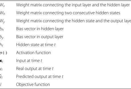
In order to improve the readability of the paper, we sum-marize the main notations that are used in the present paper in Table1:
2 Preliminaries
In this section, we review three deep learning concepts that are related to the present work: recurrent neural net-work (RNN), bi-directional RNN, and long short-term memory (LSTM).
2.1 RNN
Table 1Summary of notations
Wx Weight matrix connecting the input layer and the hidden layer
Wh Weight matrix connecting two consecutive hidden states
Wy Weight matrix connecting the hidden state and the output layer
bh Bias vector in hidden layer
by Bias vector in output layer
ht Hidden state at timet
σ (·) Activation function xt Input at timet
yt Real output at timet ˆ
yt Predicted output at timet
J Objective function
feed-forward neural networks, RNN can accommodate the temporal information embedded into the sequence of input data (see, e.g., [35,36]). Intuitively, this explains why RNN is suitable for natural language processing and time series analysis (see, e.g., [36–39]). This observation moti-vates us to leverage RNN as a starting point in designing our framework that will be presented later.
As highlighted in Fig.1, the computing process at each time step of RNN is
ht=σ(Wx·xt+Wh·ht−1+bh),
whereWx ∈ Rm×n is the weight matrix connecting the
input layer and the hidden layer withmbeing the size of the input andnbeing the size of the hidden layer,Wh ∈ Rn×n is the weight matrix between two consecutive hid-den statesht−1andht,bhis the bias vector of the hidden
layer, andσ is the activation function to generate the hid-den state. As a result, the network output can be described by
yt=σ(Wy·ht+by),
whereWy∈Rnis the weight connecting the hidden layer
and the output layer,by is the bias vector of the output
layer, andσis the activation function of the output layer.
2.2 Bi-directional RNN
A uni-directional RNN is a RNN that only takes one sequence as the input. A uni-directional RNN cannot take full advantage of the input data in the sense that it only learns information from the “past.” In order to overcome this issue, the concept of bi-directional RNN is intro-duced to make a RNN learn from both the past and the future [40]. Technically speaking, a bi-directional RNN is essentially two uni-directional RNNs that are com-bined together, where one learns from the past and the other learns from the “future”; the results of the two uni-directional RNNs are merged together to compute a final output.
2.3 LSTM
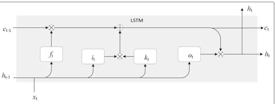
The training process of RNNs can suffer from the gradient vanishing/exploding problem [41], which can be alleviated by another RNN structure known as LSTM [42]. LSTM is composed of units calledmemory blocks, each of which contains somememory cellswith self-connections, which store (or remember) the temporal state of the network, and some special multiplicative units called gates. Each memory block contains aninput gate, which controls the flow of input activations into the memory cell; anoutput gate, which controls the output flow of cell activations into the rest of the network; and aforget gate.
As highlighted in Fig.2, the activation at stept, namely, ht, is computed based on four pieces of gate input, namely,
the information gateit, the forget gateft, the output gate
ot, and the cell gatect [43]. Specifically, the information
gate input at steptis
it=σ (Ui·ht−1+Wi·xt+bi),
whereσ(·)is a sigmoid activation function,biis the bias, xt is the input vector at stept, andWi andUiare weight
matrices. The forget gate input and the output gate input are respectively computed as
ft = σ
Uf ·ht−1+Wf ·xt+bf
, ot = σ (Uo·ht−1+Wo·xt+bo),
Fig. 2LSTM block at steptwith information gateit, forget gateft, output gateot, and cell gatect
whereUf,Uo,Wf, andWoare weight matrices, andbf and
boare biases. The cell gate input is computed as
ct=ft·ct−1+it·kt with kt=tanh(Uk·ht−1+Wk·xt+bk),
where tanh is the hyperbolic tangent function, Uk and
Wk are weights, andbk is bias. The activation at steptis
computed as
ht=ot·tanh(ct).
Intuitively, the key component of LSTM is thecell state, which flows throughout the network. Given input ht−1 andxt, theforget gate ftdecides to throw away what
infor-mation from the previous cell statect−1. The forget gateft
takesht−1andxtas input and uses the sigmoid activation
functionσ(·) to generate a number between 0 and 1 for each value in cell statect−1. The information gateit
deter-mines what new information in the current cell statectto
be stored, via two steps: a set of candidate values are com-puted byktbased on the current input; the information
gateitthen usesσ(·)to decide which candidate values will
be stored inct. The cell gate will then computect. Finally,
htis computed based onctandot, where the latter is the
information from the output gate.
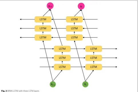
3 The bi-directional RNN with LSTM framework
The framework we propose for predicting cyber attack rates is called bi-directional RNN with LSTM or BRNN-LSTM for short, which incorporates some BRNN-LSTM layers into a bi-directional RNN. BRNN-LSTM has three com-ponents: an input layer, a number of hidden layers, and an output layer, where each hidden layer is replaced with a LSTM cell. The same sequential input, denoted byxt =
{x0, ...,xt}, is passed to the two states of the LSTM
lay-ers, the forward state, and the backward state. There is no connection in between the two states. The outputs from
the two states are then combined together to predict a tar-get value at each step. Figure3highlights the structure of BRNN-LSTM with three LSTM layers.
For training a BRNN-LSTM model, we propose using the following objective function:
J= 1 2m·
m
i=1
(yˆi−yi)2+λ
2
||W||22+ ||U||22, (1)
wheremis the size of the input,ˆyiandyiare respectively
the output of network and the observed values at stepi,
W andU are weight matrices,W = {Wf,Wi,Wk,Wo}, U= {Uf,Ui,Uk,Uo},||·||22represents the squaredL2norm of weight matrices, andλis a user-defined penalty param-eter. Note that the second term in Eq. (1) is the penalty term for avoiding overfitting. The optimization is defined as
∗=arg min
J,
where = (W,U) are model parameters and can be solved by using the gradient descent method [42,44].
4 Empirical study 4.1 Accuracy metrics
Let(y1,. . .,yN)be observed values and
ˆ
y1,. . .,yˆN
be the predicted values. In order to evaluate the accuracy of the BRNN-LSTM framework, we propose using the following widely used metrics [1,9,45].
• Mean square error (MSE): MSE=Ni=1yi− ˆyi
2
/N.
• Mean absolute deviation (MAD): MAD=Ni=1yi− ˆyi/N.
• Percent mean absolute deviation (PMAD): PMAD=Ni=1yi− ˆyi/Ni=1|yi|.
Fig. 3BRNN-LSTM with three LSTM layers
4.2 Data collection
The dataset we analyze is the same as the dataset ana-lyzed in [1]. The dataset was collected by a low-interaction honeypot consisting of 166 consecutive IP addresses dur-ing five periods of time in the interval between year 2010 and year 2011. These five periods of time are respectively 1,123, 421, 1,375, 528, and 1920 h, each of which is rep-resented by a separate dataset. The honeypot runs the following four honeypot programs: Dionaea3, Mwcollec-tor4, Amun5, and Nepenthes [46], which run some vul-nerable services such as SMB (with Microsoft Windows Server Service Buffer Overflow vulnerability MS06040 and Workstation Service Vulnerability MS06070), Net-BIOS, HTTP, MySQL and SSH. A honeypot computer runs multiple honeypot programs, each of which monitors (i.e., is associated to) one IP address. A dedicated com-puter collects the raw network traffic coming to the hon-eypot aspcapfiles. Honeypot-captured data are treated as cyber attacks because no legitimate services are associ-ated to the honeypot computers. We refer to [1] for more details about the honeypot instrument.
4.3 Data preprocessing
As in [1] and many analyses, we treat flows (rather than packets) as attacks, while noting that flows can be based
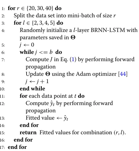
Algorithm 1Algorithm for computing fitted values. INPUT: Historical time series data{(t,yt)|t=1,. . .,m}; iterationb=10, 000; penalty parameterλ=.001.
1: forr∈ {20, 30, 40}do
2: Split the data set into mini-batch of sizer 3: forl∈ {2, 3, 4, 5}do
4: Randomly initialize al-layer BRNN-LSTM with parameters saved in
5: j←0
6: whilej<=b do
7: ComputeJin Eq. (1) by performing forward
propagation
8: Updateusing the Adam optimizer [44]
9: j←j+1
10: end while
11: foreach data point attdo
12: Computeˆytby performing forward
propagation
13: Fitted value← ˆyt
14: end for
15: return Fitted values for combination(r,l).
16: end for
17: end for
OUTPUT: Fitted values for various combinations of
(r,l)’s.
For each period or dataset, the data is represented by {(t,xt)} for t = 0, 1, 2,. . ., where xt is the number of
attacks (i.e., attack rate) that are observed by the hon-eypot at time t. Unlike [1], we further preprocess the derived attack rate time series by normalizing attack rates into interval (0, 1]. Then, small data batches (periods) are selected based on a pre-defined mini-batch size. For prediction purposes, we split each time series into an in-sample part (for model training) and an out-of-in-sample part (for prediction). As in [1], we set the last 120 h of each period as the out-of-sample part for evaluating prediction accuracy.
4.4 Model training and selection
In the training process, we use the mini-batch gradient descent method to compute the minimum of the objec-tive function, which is described in Eq. (1). We use 10,000 iterations to train a network and set the penalty param-eter λ = .001 because other parameters do not lead to any significantly better result. For each dataset, we use Algorithm 1 to compute the fitted values with varying model parameters. We select the model that achieves the minimum MSE.
Table2describes the selected model and MSE for each dataset. We observe that the selected model for different
datasets may use different batch size r and different number l of LSTM layers. For datasets I, IV, and V, the selected batch size is 20; for datasets II and III, the selected batch size is respectively 30 and 40. For the number of LSTM layers, datasets I and IV prefer to 4 layers; datasets II and V prefer to 2 layers; and period IV prefers to 3 layers.
Figure4 plots the fitting of the selected model corre-sponding to each dataset. We observe that the selected models have satisfactory fitting accuracy. In particular, the extreme values are fitted well in every dataset.
4.5 Prediction accuracy
We use Algorithm 2 to predict cyber attack rates corre-sponding to the out-of-samples, which allow us to calcu-late the prediction accuracy.
Algorithm 2Algorithm for predicting cyber attack rates INPUT: Historical time series data with in-sample set {(t,yt)|t=1,. . .,m}and out-of-sample set
{(t,ys)|s=m+1,. . .,n}; iterationb=10, 000; penalty parameterλ=.001;(r,l)selected in model training.
1: Split the in-sample set into mini-batches of sizer 2: Randomly initialize al-layer BRNN-LSTM, with all
the parameters saved in
3: j←0
4: whilej<biterationdo
5: forEach mini-batch from the in-sample setdo
6: ComputeJby performing forward propagation
7: Updateusing the Adam optimizer ([44])
8: end for
9: j←j+1
10: end while
11: Predictions← ∅
12: forEach data point,s, in the out-of-sample setdo
13: Computeyˆsby performing forward propagation
14: Predictions← ˆys
15: end for
16: return Predicted values
OUTPUT: Predicted values.
Table 3 describes the prediction results in terms of the accuracy metrics mentioned above. Based on metrics PMAD and MAPE, BRNN-LSTM achieves a remarkable prediction accuracy for datasets I, II, III, and V because prediction errors are less than 5%. However, for dataset IV, Table 2Parameters(r,l)of selected model and MSE for each dataset
Dataset I II III IV V
r 20 30 40 20 20
l 4 2 4 3 2
(a)
(b)
(c)
(d)
(e)
Fig. 4BRNN-LSTM fitting results of cyber attack rates in the five datasets (black line: observed values; red circles: fitted values)
the prediction accuracy in metric PMAD is around 17% and in metric MAPE is around 27%. Fortunately, BRNN-LSTM can be easily calibrated to improve its prediction accuracy via a rolling approach as follows. For period IV, we re-estimate model parameters in via Algorithm 1 after observing 20 more data points; the corresponding prediction accuracy, indicated by “IV*” in Table3, is much better than the original prediction accuracy. For example, the rolling approach reduces the PMAD metric to 10% and reduces the MAPE metric to 13%.
Figure5 plots the prediction results. We observe that predicted values match observed values well, but some observed values that are still missed by BRNN-LSTM. For example, for dataset III, the extreme value is missed and some observed values are over-predicted. Nevertheless, we conclude that the prediction accuracy is satisfactory.
4.6 Model comparisons
In order to further evaluate the prediction accuracy of the proposed framework, we now compare it with other popular models.
4.6.1 ARIMA
The first model we consider (as a benchmark) is the AutoRegressive Integrated Moving Average or ARIMA
(p,d,q), which is perhaps the most well-known model in time series analysis [29, 30]. The ARIMA model is described as
φ(B)(1−B)dYt=θ(B)et,
whereBis the backshift operator, andφ(B)andθ(B)are respectively the AR and MA characteristic polynomials evaluated atB. In order to select the ARIMA model for
Table 3Parameters of selected models and prediction accuracy metrics of these selected models, where IV* indicates the rolling approach for dataset IV
Dataset Test r l MSE MAD PMAD MAPE
I 120 20 4 3,628,266 463.2715 .01243741 .01387808
II 120 30 2 16,497,941 1036.6035 .04012863 .04819186
III 120 40 4 30,637,599 675.7551 .04299127 .02304677
IV 120 20 3 2,165,707 508.3557 .1658243 .26563720
IV* 120 20 3 1,085,361 297.3440 .1034426 .13385770
(a)
(b)
(c)
(d)
(e)
Fig. 5Prediction accuracy of BRNN-LSTM (black line: observed values; red circles: predicted values)
prediction purpose, we use the AIC criterion while allow-ing the orders ofpandqto vary from 0 to 5 anddto vary from 0 to 2.
4.6.2 ARMA+GARCH
The second model we consider further incorporates the Generalized AutoRegressive Conditional Heteroscedastic or GARCH model, which is widely used in financial time series applications. We use GARCH(1, 1) to model the conditional variance and the ARMA model to accommo-date the conditional mean. This leads to the following ARMA+GARCH model:
Yt=E(Yt|Ft−1)+t,
where E(·|·)is the conditional expectation function,Ft−1 is the historic information up to time t − 1, and t is the innovation of the time series. Since the mean part is modeled as ARMA(p,q), the model can be rewritten as
Yt=μ+ p
k=1
φkYt−k+
q
l=1
θlt−l+t, (2)
wheret = σtZtwithZtbeing i.i.d. innovations. For the
standard GARCH(1, 1)model, we have
σ2
t =w+α1t2−1+β1σt2−1, (3)
where σt2 is the conditional variance andwis the inter-cept. After some preliminary analysis, we set the order
of ARMA to (1, 1) as a higher order does not provide significant better predictions.
4.6.3 Hybrid model
The third model we consider is based on the recently developed hybrid approach, which is a two-step proce-dure [48, 49]. The hybrid model first extracts the linear relationship using an ARIMA model, and then uses a non-linear approach to determine the nonnon-linear relationship. The nonlinear step can be considered as a prediction on the error term. The resulting hybrid model is written as
Yt=Lt+Nt,
where Lt is the linear part andNt is the nonlinear part.
SinceLtis modeled by an ARIMA model, the residuals at
timetare
et=Yt− ˆYt,
whereYˆtis the fitted value. The residuals are modeled by
a nonlinear model, which utilizes the lag information. We consider the following three types of hybrid models:
H1 : Nt=f(et−1,et−2,. . .,et−n)+t,
H2 : Nt=f(et−1,et−2,. . .,et−n,yt−1,yt−2,. . .,yt−m)+t,
H3 : Nt=f(yt−1,yt−2,. . .,yt−n)+t,
where epsilont is the random error at time tand f is a
[50]: random Forest or RF [49], support vector machine or SVM [51], and artificial neural network or ANN [48,52].
In order to achieve the best prediction accuracy, we examine a number of models. For the linear part of ARIMA(p,d,q), we use the AIC criterion to select mod-els in the training process, wherepanddvary from 0 to 5 anddvaries from 0 to 1. For the nonlinear model, we vary the lag parameter from 1 to 12. All of the models are trained by using 10-folder validation. For RF, we set the number of trees to 1000; for SVM, we consider the follow-ing kernel functions: linear, polynomial, radial basis, and sigmoid; for ANN, we set the number of hidden layers to one while varying the number of hidden nodes from 1 to 10.
4.6.4 Comparison
We select the highest prediction accuracy in terms of the MSE metric derived from the predicted values and the out-of-sample data. For dataset I, the best predic-tion model is ARIMA(2,1,1)+ANN+H3 with the number of lags being 5 and 8 hidden nodes. For dataset II, the best prediction model is ARIMA(3,1,1)+“linear SVM”+H2 with the number of lags being 6. For dataset III, the best prediction model is ARIMA(3,0,1)+“radial SVM”+H3 with the number of lags being 8. For dataset IV, the best prediction model is ARIMA(0,1,2)+“radial SVM”+H1 with the number of lags being 4. For dataset V, the best prediction model is ARIMA+“radial SVM”+H3 with the number of lags being 7.
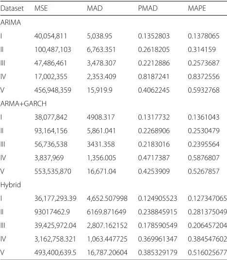
Table4summarizes the one-step ahead rolling predic-tion accuracy. Considering the MSE metric, we observe that the ARIMA model has the worst prediction accuracy for datasets I–IV, and the hybrid model outperforms the ARMA+GARCH model for every dataset; we also observe that the ARIMA model has the smallest MSE for dataset V. Considering the MAD metric, we observe that the hybrid model outperforms the other two models for datasets I, III, and IV, but the ARMA+GARCH model outperforms the other two models for dataset II; we also observe that the ARIMA model has the smallest MAD for dataset IV. Considering metrics PMAD and MAPE, we observe that the hybrid model outperforms the other two models for datasets I, III, IV, and V, and the ARMA+GARCH model is slightly better than the hybrid model for dataset II; we also observe that all of the models have the worst prediction accuracy for datasets IV and V, which coincides with the conclusion drawn in [9], namely, that the PMADs of one-step ahead rolling prediction of the FARIMA+GARCH model are respectively 0.138,0.121,0.140,0.339, and 0.378 for the five datasets. By comparing Tables 3 and 4, we draw:
Insight 1The BRNN+LSTM framework achieves a higher prediction accuracy than the FARIMA+GARCH
Table 4Prediction accuracy of the selected model with respect to each dataset
Dataset MSE MAD PMAD MAPE
ARIMA
I 40,054,811 5,038.95 0.1352803 0.1378065
II 100,487,103 6,763.351 0.2618205 0.314159
III 47,486,461 3,478.307 0.2212886 0.2573687
IV 17,002,355 2,353.409 0.8187241 0.8372556
V 456,948,359 15,919.9 0.4062245 0.5932768
ARMA+GARCH
I 38,077,842 4908.317 0.1317732 0.1361043
II 93,164,156 5,861.041 0.2268906 0.2530479
III 56,736,538 3431.358 0.2183016 0.2395564
IV 3,837,969 1,356.005 0.4717387 0.5876807
V 553,535,870 16,671.04 0.4253909 0.5267857
Hybrid
I 36,177,293.39 4,652.507998 0.124905523 0.127347065
II 93017462.9 6169.871649 0.238845915 0.281375049
III 39,425,972.04 2,807.162152 0.178590549 0.206457204
IV 3,162,758.321 1,063.447725 0.369961347 0.384547602
V 493,400,639.5 16,787.20604 0.385329179 0.516025677
model proposed in [9] and the ARIMA, ARIMA+GARCH, and hybrid models considered above.
5 Conclusion
We proposed a BRNN-LSTM framework for predict-ing cyber attack rates. The framework can accommo-date complex phenomena exhibited by datasets, including long-range dependence and highly nonlinearity. Using five real-world datasets, we showed that the framework sig-nificantly outperforms the other prediction approaches in terms of prediction accuracy, which confirms that LSTM cells can indeed accommodate the long memory behav-ior of cyber attack rates. From these five datasets, we found that only dataset IV requires to re-training the model in order to achieve a better prediction accuracy. We compared the prediction accuracy of BRNN-LSTM and other prediction approaches, which use rolling predic-tions (i.e., re-building the prediction model after observ-ing a new value). We hope the present work will inspire more research in deploying deep learning to prediction tasks in the cybersecurity domain.
Endnotes
1
https://www.symantec.com/security-center/threat-report
2
3http://dionaea.carnivore.it/
4https://alliance.mwcollect.org/
5http://amunhoney.sourceforge.net/
Abbreviations
ARIMA: Autoregressive integrated moving average; BRNN: Bi-directional recurrent neural network; GARCH: Generalized autoregressive conditional heteroskedasticity; LSTM: Long short-term memory; RNN: Recurrent neural network
Acknowledgements Not applicable.
Funding Not applicable.
Availability of data and materials
Data used in this work is not suitable for public use. The source code used in the present paper is available at https://github.com/xingfang912/time-series-analysis
Competing interests
The authors declare that they have no competing interests.
Authors’ contributions
XF constructed the deep learning framework and performed the deep learning experiments. MX and PZ performed the experiments on the statistical models. SX drafted the manuscript. All authors reviewed the draft. All authors read and approved the final manuscript.
Publisher’s Note
Springer Nature remains neutral with regard to jurisdictional claims in published maps and institutional affiliations.
Author details
1School of Information Technology, Illinois State University, Normal 61761, IL, USA.2Department of Mathematics, Illinois State University, Normal 61761, IL, USA.3Department of Computer Science, University of Texas at San Antonio, San Antonio 78249, TX, USA.4Department of Computer Science, Jiangsu Normal University, Xuzhou 221110, China.
Received: 29 November 2018 Accepted: 3 May 2019
References
1. Z. Zhan, M. Xu, S. Xu, Characterizing honeypot-captured cyber attacks: Statistical framework and case study. IEEE Trans. Inf. Forensic Secur.8(11), 1775–1789 (2013)
2. E. Gandotra, D. Bansal, S. Sofat, Computational techniques for predicting cyber threats. Intell. Comput. Commun. Devices Proc ICCD 2014.1, 247 (2014)
3. S. Xu, inProc. Symposium on the Science of Security (HotSoS’14). Cybersecurity dynamics (ACM, Raleigh, 2014), pp. 14–1142 4. S. Xu, inProactive and Dynamic Network Defense, ed. by Z. Lu, C. Wang.
Cybersecurity dynamics: A foundation for the science of cybersecurity (Springer International Publishing, New York City, 2018)
5. L. D. Carli, R. Sommer, S. Jha, inProceedings of the 2014 ACM SIGSAC Conference on Computer and Communications Security, Scottsdale, AZ, USA, November 3-7, 2014. Beyond pattern matching: A concurrency model for stateful deep packet inspection (ACM, Scottsdale, 2014), pp. 1378–1390 6. C. Ishida, Y. Arakawa, I. Sasase, K. Takemori, inProceedings of PACRIM. 2005
IEEE Pacific Rim Conference on Communications, Computers and signal Processing, August 24-26. Forecast techniques for predicting increase or decrease of attacks using bayesian inference (IEEE, Victoria, 2005), pp. 450–453
7. D. H. Kim, T. Lee, S.-O. D. Jung, H. P. In, H. J. Lee, inInformation Assurance and Security, 2007. IAS 2007. Third International Symposium On. Cyber threat trend analysis model using HMM (IEEE, Manchester, 2007), pp. 177–182
8. Z. Yong, T. Xiaobin, X. Hongsheng, inComputational Intelligence and Security, 2007 International Conference On. A novel approach to network security situation awareness based on multi-perspective analysis (IEEE, Harbin, 2007), pp. 768–772
9. Z. Zhan, M. Xu, S. Xu, Predicting cyber attack rates with extreme values. IEEE Trans. Inf. Forensic Secur.10(8), 1666–1677 (2015)
10. C. Peng, M. Xu, S. Xu, T. Hu, Modeling and predicting extreme cyber attack rates via marked point processes. J. Appl. Stat.44(14), 2534–2563 (2017) 11. M. Xu, L. Hua, S. Xu, A vine copula model for predicting the effectiveness of cyber defense early-warning. Technometrics.59(4), 508–520 (2017) 12. C. Peng, M. Xu, S. Xu, T. Hu, Modeling multivariate cybersecurity risks. J.
Appl. Stat.45(15), 2718–2740 (2018)
13. N. Sun, J. Zhang, P. Rimba, S. Gao, Y. Xiang, L. Y. Zhang, Data-driven cybersecurity incident prediction: A survey. IEEE Commun. Surv. Tutor., 1–1 (2018).https://doi.org/10.1109/COMST.2018.2885561
14. M. Husák, J. Komárková, E. Bou-Harb, P. ˇCeleda, Survey of attack projection, prediction, and forecasting in cyber security. IEEE Commun. Surv. Tutor.21(1), 640–660 (2019)
15. D. E. Denning, An intrusion-detection model. IEEE Trans. Softw. Eng. SE-13(2), 222–232 (1987)
16. M. Markou, S. Singh, Novelty detection: a review part 1: statistical approaches. Sig. Process.83(12), 2481–2497 (2003)
17. V. Chandola, A. Banerjee, V. Kumar, Anomaly detection: a survey. ACM Comput. Surv. (CSUR).41(3), 15 (2009)
18. J. Neil, C. Hash, A. Brugh, M. Fisk, C. B. Storlie, Scan statistics for the online detection of locally anomalous subgraphs. Technometrics.55(4), 403–414 (2013)
19. L. Deng, D. Yu, et al., Deep learning: methods and applications. Found. Trends® Sig. Process.7(3–4), 197–387 (2014)
20. M. Längkvist, L. Karlsson, A. Loutfi, A review of unsupervised feature learning and deep learning for time-series modeling. Pattern Recogn. Lett.42, 11–24 (2014)
21. R. C. Cavalcante, R. C. Brasileiro, V. L. Souza, J. P. Nobrega, A. L. Oliveira, Computational intelligence and financial markets: A survey and future directions. Expert Syst. Appl.55, 194–211 (2016)
22. D. Li, Q. Li, Y. Ye, S. Xu, Enhancing robustness of deep neural networks against adversarial malware samples: Principles, framework, and aics’2019 challenge. CoRR.abs/1812.08108(2018).http://arxiv.org/abs/1812. 08108
23. D. Li, R. Baral, T. Li, H. Wang, Q. Li, S. Xu, Hashtran-dnn: a framework for enhancing robustness of deep neural networks against adversarial malware samples. CoRR.abs/1809.06498(2018).http://arxiv.org/abs/ 1809.06498
24. Z. Li, D. Zou, S. Xu, X. Ou, H. Jin, S. Wang, Z. Deng, Y. Zhong, in25th Annual Network and Distributed System Security Symposium, NDSS 2018, San Diego, California, USA, February 18-21, 2018. Vuldeepecker: A deep learning-based system for vulnerability detection (Internet Society, San Diego, 2018) 25. Z. Li, D. Zou, S. Xu, H. Jin, Y. Zhu, Z. Chen, S. Wang, J. Wang, Sysevr: A
framework for using deep learning to detect software vulnerabilities. CoRR.abs/1807.06756(2018).http://arxiv.org/abs/1807.06756 26. G. Grieco, G. L. Grinblat, L. Uzal, S. Rawat, J. Feist, L. Mounier, inProceedings
of the Sixth ACM Conference on Data and Application Security and Privacy. CODASPY ’16. Toward large-scale vulnerability discovery using machine learning (ACM, New York, 2016), pp. 85–96
27. Z. Li, D. Zou, S. Xu, H. Jin, H. Qi, J. Hu, inProceedings of the 32nd Annual Conference on Computer Security Applications, ACSAC 2016, Los Angeles, CA, USA, December 5-9, 2016. Vulpecker: an automated vulnerability detection system based on code similarity analysis (ACM, Los Angeles, 2016), pp. 201–213
28. Y. Chen, M. Khandaker, Z. Wang, inProceedings of the 2017 ACM on Asia Conference on Computer and Communications Security. ASIA CCS ’17. Pinpointing vulnerabilities (ACM, New York, 2017), pp. 334–345 29. J. D. Cryer, K.-S. Chan,Time Series Analysis With Applications in R. (Springer,
New York, 2008)
30. P. J. Brockwell, R. A. Davis,Introduction to Time Series and Forecasting. (Springer, Switzerland, 2016)
31. J. Ke, H. Zheng, H. Yang, X. M. Chen, Short-term forecasting of passenger demand under on-demand ride services: A spatio-temporal deep learning approach. Transp. Res. C Emerg. Technol.85, 591–608 (2017) 32. M. Barabas, G. Boanea, A. B. Rus, V. Dobrota, J. Domingo-Pascual, in
International Conference On. Evaluation of network traffic prediction based on neural networks with multi-task learning and multiresolution decomposition (IEEE, Cluj-Napoca, 2011), pp. 95–102
33. A. Azzouni, G. Pujolle, A Long Short-Term Memory Recurrent Neural Network Framework for Network Traffic Matrix Prediction. CoRR. abs/1705.05690(2017).http://arxiv.org/abs/1705.05690
34. S. Siami-Namini, A. S. Namin, Forecasting Economics and Financial Time Series: ARIMA vs. LSTM. CoRR.abs/1803.06386(2018).http://arxiv.org/ abs/1803.06386
35. C.-M. Kuan, T. Liu, Forecasting exchange rates using feedforward and recurrent neural networks. J. Appl. Econ.10(4), 347–364 (1995) 36. T. Mikolov, M. Karafiát, L. Burget, J. Cernocký, S. Khudanpur, inProceesings
of the 11th Annual Conference of the International Speech Communication Association. Recurrent neural network based language model (International Speech Communication Association (ISCA), Makuhari, Chiba, 2010), pp. 1045–1048
37. M. Sundermeyer, I. Oparin, J. L. Gauvain, B. Freiberg, R. Schlüter, H. Ney, in 2013 IEEE International Conference on Acoustics, Speech and Signal Processing. Comparison of feedforward and recurrent neural network language models (IEEE, Vancouver, 2013), pp. 8430–8434
38. Z. Huang, G. Zweig, B. Dumoulin, in2014 IEEE International Conference on Acoustics, Speech and Signal Processing (ICASSP). Cache based recurrent neural network language model inference for first pass speech recognition (IEEE, Florence, 2014), pp. 6354–6358
39. X. Liu, Y. Wang, X. Chen, M. J. Gales, P. C. Woodland, inAcoustics, Speech and Signal Processing (ICASSP), 2014 IEEE International Conference On. Efficient lattice rescoring using recurrent neural network language models (IEEE, Florence, 2014), pp. 4908–4912
40. M. Schuster, K. K. Paliwal, Bidirectional recurrent neural networks. IEEE Trans. Sig. Process.45(11), 2673–2681 (1997)
41. Y. Bengio, P. Simard, P. Frasconi, Learning long-term dependencies with gradient descent is difficult. IEEE Trans. Neural Netw.5(2), 157–166 (1994) 42. S. Hochreiter, J. Schmidhuber, Long short-term memory. Neural Comput.
9(8), 1735–1780 (1997)
43. I. Goodfellow, Y. Bengio, A. Courville,Deep Learning. (MIT Press, MA, 2016) 44. D. P. Kingma, J. Ba, Adam: A method for stochastic optimization. CoRR.
arXiv preprint arXiv:1412.6980(2014)
45. R. J. Hyndman, A. B. Koehler, Another look at measures of forecast accuracy. Int. J. Forecast.22(4), 679–688 (2006)
46. P. Baecher, M. Koetter, T. Holz, M. Dornseif, F. Freiling, inInternational Workshop on Recent Advances in Intrusion Detection. The nepenthes platform: An efficient approach to collect malware (Springer, Berlin, Heidelberg, 2006), pp. 165–184
47. S. Almotairi, A. Clark, G. Mohay, J. Zimmermann, in2008 IFIP International Conference on Network and Parallel Computing. Characterization of attackers’ activities in honeypot traffic using principal component analysis (IEEE, Shanghai, 2008), pp. 147–154
48. G. P. Zhang, Time series forecasting using a hybrid arima and neural network model. Neurocomputing.50, 159–175 (2003)
49. M. Kumar, M. Thenmozhi, Forecasting stock index returns using arima-svm, arima-ann, and arima-random forest hybrid models. Int. J. Bank. Account. Financ.5(3), 284–308 (2014)
50. J. Friedman, T. Hastie, R. Tibshirani,The Elements of Statistical Learning, vol. 1. (Springer, New York, 2001)
51. P.-F. Pai, C.-S. Lin, A hybrid arima and support vector machines model in stock price forecasting. Omega.33(6), 497–505 (2005)