Development of a Simulator for Plasma Position
and Shape Control in JT-60SA
Yoshiaki MIYATA, Takahiro SUZUKI, Takaaki FUJITA, Shunsuke IDE and Hajime URANO
Japan Atomic Energy Agency, 801-1 Mukoyama, Naka, Ibaraki 311-0193, Japan (Received 3 February 2012/Accepted 14 July 2012)
A simulator has been developed to control the position and shape of plasmas. It consists of an equilibrium solver and an “isoflux” controller. The equilibrium solver identifies an equilibrium under the specified poloidal field (PF) coil current and incorporates the effect of eddy currents. The plasma position and shape are obtained as a result of the equilibrium calculation by an introducing the imaginary magnetic field. The controller enables the simulation of the control of the position and shape using the isoflux technique and optimizes the control logic of the coil current in JT-60SA. It also controls the PF coil currents such that the poloidal flux remains equal at all specified locations. The simulation of the control of the position and shape in response to prescribed changes in the configuration, internal parameters, poloidal beta, and internal inductance is demonstrated. The transition from a limiter to a divertor configuration is also simulated.
c
2012 The Japan Society of Plasma Science and Nuclear Fusion Research
Keywords: JT-60SA, plasma position and shape control, control logic, poloidal field coil, equilibrium solver, isoflux controller
DOI: 10.1585/pfr.7.1405137
1. Introduction
Control of the plasma position and shape is an im-portant issue for JT-60SA [1, 2], ITER, and DEMO, which have a small number of coils. The precise control of the plasma position is critical for avoiding damages to plasma facing components, such as the first wall. Therefore, the simulation of the control of the plasma position and shape in JT-60SA is being studied to predict the controllability of the ITER and DEMO [3, 4] plasmas. The results of the plasma control studies for JT-60SA will contribute to a control scheme and suitable operational regimes for ITER and DEMO.
Several methods for controlling the plasma position and shape have been applied in tokamak machines [5], and the following two are used in the control system in this study. The first method is the “isoflux” technique [6], which controls the last closed flux surface. The isoflux control scheme has been applied to the shape control sys-tem of DIII-D [7] using the RTEFIT algorithm [8]. The second method is the direct control of the plasma shape parameters, which is used for JT-60U [9], ASDEX-U [10], and JET [11].
In JT-60U, there are 43 separate copper poloidal field (PF) coils connected in series as five independently pow-ered PF coil sets. They provide the poloidal flux (F coil set), the vertical field (VR coil set), the horizontal field (H coil set), the divertor field (D coil set), and a field to con-trol the plasma cross-sectional triangularity (VT coil set) in the highly elongated mode. The JT-60U control sys-tem operates by controlling five control parameters with author’s e-mail: [email protected]
the five coil sets. These controlled parameters include the plasma current (IP), the radial plasma position (R), the ver-tical plasma position (Z), the height of the X-point from the divertor (XP), and the triangularity (δ), and they are primarily controlled by the F, VR, H, D, and VT coil sets, respectively. The plasma current, position, and shape are reproduced in real time using the Cauchy Condition Sur-face (CCS) method [12] and are directly utilized for feed-back control.
The JT-60SA device is capable of confining break-even-equivalent class high-temperature plasmas lasting for a duration longer than the time scales characterizing key plasma processes. To do so, superconducting toroidal and PF coils are used for plasma control. Advanced control logic is necessary, because the magnetic field for plasma control cannot be produced solely by each superconducting coil in JT-60SA. Thus, the isoflux technique is employed for the control of the position and shape of the plasma in JT-60SA. The isoflux technique is described in detail in Sec. 2.2.
In JT-60SA, there are 10 PF coils and 2 fast plasma position control coils (FPPCCs). The PF coils and FP-PCCs are superconducting and in-vessel copper coils, re-spectively. The PF coils consist of central solenoid (CS) modules and equilibrium field (EF) coils. Because of the rapid changes in the plasma position and shape, an inte-grated control method using both the PF coils and FPPCCs is necessary. In addition, because the Since JT-60SA plas-mas are placed close to the stabilizing wall for higher sta-bility, accurate position control is necessary to prevent the plasma from touching the wall. The eddy currents induced
c
2012 The Japan Society of Plasma
at the conducting elements, which consist of the vacuum vessel (VV) and the stabilization plate (SP), make a cer-tain contribution to the equilibrium, and thus to the coil current distribution also, particularly during the ramp-up and down phases. The feedback controller controls the last closed flux surface in reference to the plasma position and shape reproduced in real time by the CCS method. There-fore, the simulation of the control of the plasma position and shape is necessary to optimize the control logic of the coil current.
Because of the large eddy currents in the VV in JT-60SA, it is necessary for the control logic to incorporate the effect of shielding of the magnetic field. Thus, a posi-tion and shape control simulator that incorporates the ef-fect of eddy currents was developed for the exploration of techniques to control the plasma position and shape. Pro-portional (P)–integral (I)–derivative (D) feedback control based on the isoflux technique is used in the control simu-lator. With this new system, it is possible to simulate the control of the position and shape using the isoflux tech-nique and optimize the control logic of the coil current in JT-60SA. In the future, the control simulator will be used in combination with the CCS method.
In Sec. 2, an outline of the control simulator is pro-vided. In Sec. 3, the control of the position and shape is been simulated in response to prescribed changes in the configuration and plasma internal parameters. A summary is described in Sec. 4.
2. Outline of the Control Simulator
The simulator consists of an equilibrium calculation component and a controller component. The plasma equi-librium for a given set of coil currents is obtained from the equilibrium calculation component. The set of coil cur-rents is modified to adjust the plasma position and shape for the next time step in the controller component. By iter-ating these procedures, the feedback control of the plasma position and shape is simulated by controlling the coil cur-rent. The control logic of the coil current is also optimized using the simulator.2.1
Equilibrium calculation component
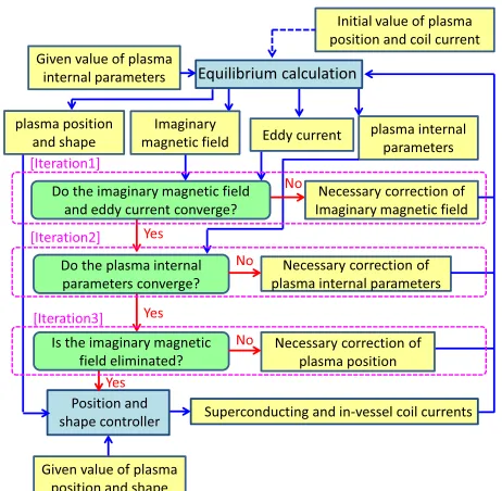
Figure 1 shows the calculation flow. In a usual equi-librium code (e.g., TOSCA) [13], the plasma position and shape are given, and the coil current is adjusted to obtain the equilibrium for a given position and shape. TOSCA is a free-boundary equilibrium analysis code that is suit-able for designing tokamak experiments. In this code, the Grad–Shafranov equation for tokamak plasmas is solved. On the other hand, in the equilibrium calculation compo-nent of the simulator, the plasma position and shape are ob-tained as a result of an equilibrium calculation. However, the control simulator is developed, for which an imaginary magnetic field was introduced, on the basis of the TOSCA code. The plasma position is assumed, and the equilibrium
Fig. 1 Calculation flow of the control simulator. It consists of an equilibrium calculation component and the controller component. By iterating these procedures, the feedback control of the plasma position and shape is simulated by controlling the coil current.
is calculated by adjusting the imaginary field, which was defined as a uniform field using the following equations;
ΨV= μ0 Ictl1 2aV
(R2−RV2),
ΨH=
μ0Ictl2 aV
RVZ, (1)
then, BZ =
1 R
∂
∂R(ΨV+ΨH)=
μ0Ictl1 aV ,
BR=− 1 R
∂
∂Z(ΨV+ΨH)=−
μ0Ictl2 aV
RV
R , (2)
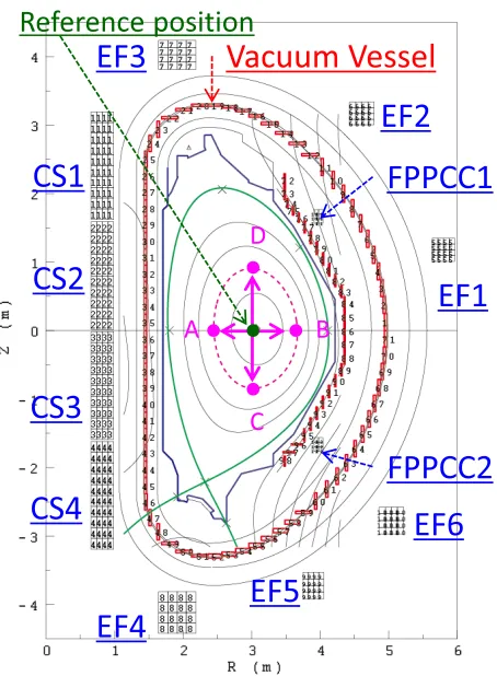
Fig. 2 Locations of the reference position, fixed points, PF coils, in-vessel coils, and toroidal conducting elements in JT-60SA. Four fixed points (A–D) were established at a dis-tance from the reference position. The PF coils consist of 4 CS modules and 6 EF coils.
directions of the coil and eddy currents are defined in a manner similar to the plasma current. The poloidal flux in the plasma is described as the decreasing function of the minor radius. Figure 2 shows the locations of the refer-ence position, fixed points, PF coils, in-vessel coils, and toroidal conducting elements in JT-60SA. The VV and SP are modeled as 71 and 27 toroidal conducting elements, respectively. The primary function of the SP is to increase the ideal beta limit and improve the plasma positional sta-bility.
The imaginary magnetic field current is adjusted such that the total poloidal flux remains equal at the fixed points in the horizontal and vertical directions. The imaginary magnetic field currents that are necessary for the total poloidal flux to be equal at points A and B are given by
Ψ(A)+ΨV(A)=Ψ(B)+ΨV(B), (3) and those necessary for the total poloidal flux to be equal at points C and D are given by
Ψ(C)+ΨH(C)=Ψ(D)+ΨH(D). (4) The poloidal fluxΨis defined as
Ψ=ΨP+ΨC+ΨE, (5) whereΨP,ΨC, andΨE are the poloidal flux produced by
Fig. 3 Waveforms of the equilibrium calculation using “Itera-tion 1” and “Itera“Itera-tion 2”; (a) the root mean square (RMS) of the eddy current, (b) the necessary imaginary mag-netic field current in the horizontal and vertical directions, (c) the internal inductance, and (d) the poloidal beta. The horizontal axis indicates the iteration counts of the equi-librium calculation.
the plasma, coil, and eddy currents, respectively. Thus, it is possible to calculate the poloidal flux using the Green function in the control simulator.
With Eq. (1) we have Ictl1=−
2aV·(Ψ(B)−Ψ(A))
μ0·(RB2−RA2) , Ictl2=−
aV·(Ψ(D)−Ψ(C))
μ0·(ZD−ZC) ,
field, the plasma internal parameters (internal inductance and poloidal beta) are also fixed to the given values by ad-justing the plasma pressure and current profile as shown in Figs. 3 (c) and 3 (d).
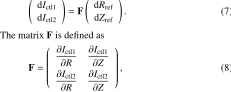
The plasma position is adjusted to minimize the imag-inary magnetic field, and then the equilibrium realized for a given set of coil currents is obtained. The relationship between the displacement of the reference position and the change in the magnetic field current is used to adjust the plasma position. The relationship can be presented as
dIctl1 dIctl2 =F dRref dZref . (7)
The matrixFis defined as
F= ⎛ ⎜⎜⎜⎜⎜ ⎜⎜⎜⎜⎜ ⎜⎝
∂Ictl1
∂R
∂Ictl1
∂Z
∂Ictl2
∂R
∂Ictl2
∂Z ⎞ ⎟⎟⎟⎟⎟ ⎟⎟⎟⎟⎟
⎟⎠, (8)
where dIctl1 and dIctl2 are the changes in the imaginary magnetic field current in the vertical and horizontal direc-tions, respectively, and dRrefand dZrefare the displacement of the horizontal and vertical reference positions to be cor-rected, respectively. The matrixFconsists of the partial differential coefficient that indicates the perturbation of the imaginary magnetic field current per unit displacement in the horizontal and vertical directions. It is obtained by cal-culating three different equilibrium solutions with the nec-essary imaginary magnetic field currents for different ref-erence positions moved in the horizontal and vertical di-rections. Then, Eq. (7) can be rewritten as
dRref dZref
=F−1
dIctl1 dIctl2
, (9)
whereF−1is the inverse of matrixF. By substituting the imaginary magnetic field current into the right-hand side of Eq. (9), we obtain the necessary correction for the ref-erence position. Figure 4 shows the waveforms of the equilibrium calculation using “Iteration 3” in Fig. 1. The horizontal axis indicates the iteration count of “Iteration 3”. “Iteration 3” calculates the necessary correction of the plasma position. HereRref andZrefare the horizontal and vertical reference positions, respectively. The controlled plasmaIP=5.5 MA, the internal inductanceli=0.75, and the poloidal betaβP=0.74 with the divertor configuration. The necessaryIctl1 andIctl2are approximately 14 kA and 4 kA at the desired initial reference positionsRref =3.0 m andZref =0.0 m, respectively. Then, the plasma position was adjusted on the basis of the necessary correction of the horizontal and vertical reference positions calculated from Eq. (9). After repeating this procedure three times, the dis-placement of the reference positions was less than the con-vergence condition (dRrefand dZref<10−4m). The neces-saryIctl1andIctl2approximately became 0.4 mA and 7 mA at the reference positionsRref =3.07 m andZref=0.03 m, respectively. Thus, the plasma position and shape for a given set of coil currents were obtained because the
imag-Fig. 4 Waveforms of the equilibrium calculation using “Itera-tion 3”; (a) the horizontal and vertical reference posi“Itera-tions, (b) the displacement of the horizontal and vertical refer-ence positions, and (c) the imaginary magnetic field cur-rent. The horizontal axis indicates the iteration counts for adjusting the reference position.
inary magnetic field current was eliminated.
2.2
Controller component
The isoflux technique is employed for the control of the position and shape in JT-60SA. A set of locations that defines the desired plasma separatrix is specified as the control points. The PF coil currents are adjusted to main-tain an equal poloidal flux at the X or limiter point. The small difference between the flux at the control points and its reference value is defined asδΨ. The relationship be-tween the changes in the coil currentsδIandδΨcan be represented asδI = M−1δΨ. TheM−1 is the control ma-trix that is the generalized inverse of the Green function M calculated using the singular value decomposition method. The Green function M represents the poloidal flux at each control point per unit current.
For the PF coils, the P-I feedback control is used in the relationship betweenδIandδΨ. The controller modifies the PF coil currents according to the following equation,
I(t+ Δt) =I(t0)+MPF−1
GSP{δΨS(t)}+GSI t
t0
δΨS(t)dt
+GXP{dΨX(t)}+GXI t
t0
{dΨX(t)}dt
. (10)
TheδΨSand dΨXare defined as
δΨS(t)= ⎛ ⎜⎜⎜⎜⎜ ⎜⎜⎜⎜⎜ ⎜⎜⎜⎜⎜ ⎜⎝ 0
ΨX(t)−ΨP1(t)
... ΨX(t)−ΨPn(t)
dΨX(t)= ⎛ ⎜⎜⎜⎜⎜ ⎜⎜⎜⎜⎜ ⎜⎜⎜⎜⎜ ⎜⎝
ΨX(t−1)−ΨX(t) 0
...
0
⎞ ⎟⎟⎟⎟⎟ ⎟⎟⎟⎟⎟ ⎟⎟⎟⎟⎟ ⎟⎠
, (11)
where δΨS is the n vector of the difference between the reference flux value and the flux at the control point, and n is the number of control points; the first control point is an X or limiter point, and the flux there is used as the reference value, and the 1st row δΨS is zero; ΨX is the nvector of the flux, where the first element is the flux at the first control point, and the elements from the 2nd to the (n+1)th rows are zero;t0andΔtare the initial time and the control cycle, respectively.Iis themvector of the PF coil currents;MPF−1is the (m×(n+1)) control matrix, wherem is the number of PF coils;GSPandGSIare, respectively, the control gain of the PI feedback controls that are necessary to make the poloidal flux equal at all control points; and GXP andGXI are, respectively, the control gains of the PI feedback controls necessary to maintain the poloidal flux at its initial value at the X point. The units of the parameters are as follows: δΨSandΨXare in webers,t0 andΔtare in seconds,Iis in amperes,GSPandGXPare in 1, andGSI andGXIin 1/s.
The controller modifies the FPPCC currents with ref-erence to the diffref-erence between the refref-erence flux value and the flux value at the two desired control points. These points are chosen to control the two FPPCCs. The FPPCCs are used for transient control, and their DC currents should be zero over longer time scales. For the FPPCCs, the D feedback control is used in the relationship betweenδIand
δΨ. The controller modifies the two FPPCC currents ac-cording to the following equation;
I(t+ Δt)=GFDMFPC−1 d
dtδΨS(t), (12) where,δΨSis the two vectors for the difference between the reference flux and the flux value at the desired two control points;GFD is the control gain of the D feedback control (in s), andMFPC−1is the (2×2) control matrix.
3. Simulation Results
The control of the position and shape has been sim-ulated during the transition from the limiter to the diver-tor configuration and during the heating phase in JT-60SA. The following two examples are simulated as test cases, and the control logic is not optimized. The control logic will be optimized using the control simulator in the future. The given reference values of the plasma parameters, ini-tial coil currents and eddy currents, are necessary to simu-late the control of the position and shape as follows: (1) starting/ending time, calculation cycles, coil control cy-cles, convergence conditions, initial reference positions; (2) initial values of the plasma internal parameters, plasma current profile parameters, coil currents, and eddy currents; (3) waveforms of the reference values of the plasma
inter-nal parameters; and
(4) waveforms of the position and number of control points and control gains.
The initial values of the plasma internal parameters, plasma current profile parameters, coil currents, and eddy currents are given in the TOSCA code.
3.1
Plasma shape transition
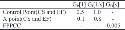
The control of the position and shape has been sim-ulated during the transition from a limiter to a divertor configurations. The controlled plasma parameters are as follows: plasma currentIP =587 kA, internal inductance li = 0.84, and poloidal beta βP = 0.10. It is impossi-ble to simultaneously control both the plasma shape and plasma current. The plasma current, internal inductance and poloidal beta are fixed to the initial value during the transition from the limiter to the divertor configuration, and the plasma current profile is adjusted to fix the poloidal beta and internal inductance to the given values. In the fu-ture, the control simulator will incorporate theIP control logic. All the equilibrium calculation cycles and control cycles of the PF coils and FPPCCs are 20 ms. The values of control gains are shown in Table 1. Figures 5 and 6 show the simulation results during the transition from a limiter to a divertor configuration. The six initial input control points (P0–P5) served as the references for the position and shape. Point P0 is the limiter point. The number of input control points was increased from 6 to 9 (including the X point) att = 7.02 s as shown in Fig. 5. The controller modified the CS and EF currents to adjust the flux at the control points and FPPCC currents with reference to the flux at P1 and P2. Points P1 and P2 were considered appropriate for the horizontal and vertical controls, respectively. The dis-placementdbetween the separatrix and a control point can be presented as
d= ΨP−ΨX
|∇ΨP| ,
(13) whereΨP is the flux at a control point andΨXis the flux of the X point. A displacement in the positive direction indicates that the separatrix is outside the control point. The units of the parameters are as follows: dis in meters, andΨPandΨXare in webers.
The transition from a limiter to a divertor configura-tion was made in two steps: (1) an increase of the elon-gation, and (2) formation of the X point. The coil voltage was evaluated by summing the time derivative of the fluxes produced by all the coils, conducting elements, and plasma
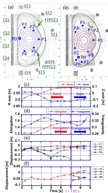
Fig. 5 Simulation results during the transition from the limiter to the divertor configuration. (a) Equilibrium configuration (blue solid lines) with 6 initial control points. (b) Equilib-rium configuration (red solid lines) with 9 control points att =8.6 s. Waveforms of (c) the horizontal and verti-cal positions of the magnetic axis, (d) the elongation and triangularity of the last closed flux surface, (e) the dis-placement between the separatrix and the control points (P1–P4) and (f) the displacement between the separatrix and the control points (P5–P8).
at each coil. Figure 7 shows the contour of the eddy cur-rent profile, which was induced in the conducting elements around the plasma.
Points P2–P5 were moved in a vertical direction from t = 3.0 to 5.0 s to increase the elongation. As a result, the elongation was increased from approximately 1.23 to 1.48 as the plasma shape changed (the last closed flux sur-face) to follow the control points as shown in Fig. 5 (d). The EF2 and EF5 currents decreased (in the negative di-rection) to increase the elongation, as shown in Fig. 6 (b). Meanwhile, the EF1 current decreased (in the positive di-rection) to complement the change in the flux produced by
Fig. 6 Simulation results during the transition from the limiter to the divertor configuration. Waveforms of (a) the CS1– CS4 coil currents, (b) EF1, EF2, EF5, and EF6 currents, (c) the EF3 and EF4 currents, (d) the FPPCC1 and FP-PCC2 currents, (e) the CS1–CS4 voltages, (f) the EF1– EF6 voltages, and (g) the FPPCC1 and FPPCC2 voltages.
lim-Fig. 7 Contour of the eddy current profile. The conductor num-ber corresponds to the upper outboard VV (#1–#20), in-board VV (#21–#51), lower outin-board VV (#52–#71), and SP (#72–#98). Control points P2–P5 were moved in a vertical direction fromt=3 to 5 s to increase the elonga-tion. The P8 control point was moved in a vertical direc-tion to form of the X point beginning att=7.02 s.
iter to a divertor configuration was possible by changing the number and positions of the control points. The capa-bility for the early formation of a divertor configuration is preferable.
3.2
Plasma internal parameter changes
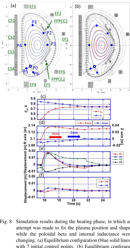
Control of the position and shape was also simu-lated during the heating phase, in which an attempt was made to maintain a constant position and shape of the plasma, while the poloidal beta and internal inductance were changed. Normally, the plasma position changes in response to changes in the poloidal beta and internal in-ductance. The changes in the poloidal beta and internal inductance occur not only at the start/end of the heating phase, but also during certain MHD activities and the re-sulting collapse, during the ramp–up and down phases of theIP, at sudden L/H or H/L transitions, during ITB for-mation among others. The parameters of the controlled plasma in the simulation were as follows: IP = 5.5 MA, initial internal inductanceli = 0.84, and initial poloidal beta βP = 0.50. All the equilibrium calculation cycles and the control cycles of the PF coils and FPPCCs were 20 ms. Figures 8 and 9 show the simulation results during the heating phase, in which an attempt was made to main-tain a fixed position and shape of the plasma, while the poloidal beta and internal inductance were changed. Six input control points (P1–P6) served as the references for the position and shape. Figure 10 shows the contour of the eddy current profile, that was induced in the conducting elements around the plasma.
The plasma position and shape were fixed at the re-quired values according to the operational scenario. As
Fig. 8 Simulation results during the heating phase, in which an attempt was made to fix the plasma position and shape, while the poloidal beta and internal inductance were changing. (a) Equilibrium configuration (blue solid lines) with 7 initial control points. (b) Equilibrium configura-tion (red solid lines) with 7 control points att=21.6 s. Waveforms of (c) the poloidal beta and internal induc-tance, (d) the horizontal and vertical positions of the mag-netic axis, (e) the displacement between the separatrix and the control points (P1–P4), and (f) the displacement between the separatrix and the strike points (P5, P6).
shown in Fig. 8 (c), the poloidal beta increased exponen-tially from approximately 0.5 to 0.75 with a time con-stant of 1 s, which corresponds to the energy confinement time. Meanwhile, the internal inductance decreased learly from approximately 0.85 to 0.75 with time. The in-ternal parameters were converged at each time step.
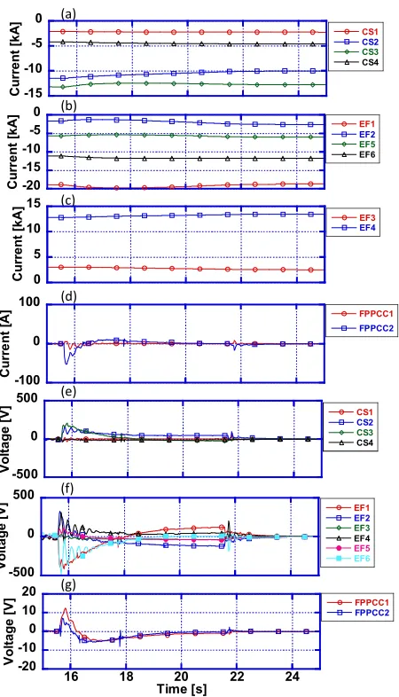
sup-Fig. 9 Simulation results during the heating phase, in which an attempt was made to fix the plasma position and shape, while the poloidal beta and internal inductance were changing. Waveforms of (a) the CS1–CS4 coil currents, (b) the EF1, EF2, EF5 and EF6 currents, (c) the EF3 and EF4 currents, (d) the FPPCC1 and FPPCC2 currents, (e) the CS1–CS4 voltages, (f) the EF1–EF6 voltages, and (g) the FPPCC1 and FPPCC2 voltages.
ported the rapid change in the plasma position and shape, as can be seen in Fig. 9 (d). Positive eddy currents were induced in the outboard of the VV because of changes in the magnetic field produced by the EF1 and EF6 cur-rents. It is important to note that the coil voltages must be limited within the power supply capacities, as shown in Fig. 9. The limits of EF1 and EF6 currents were−20 kA, and+10 kA, respectively, while the limit of EF1 and EF6 voltages was±1 kV. Therefore, the EF1 and EF6 currents and voltages were within the limits of the current and volt-age. It should be noted that these limits create limitations for the heating/βPwaveform. The separatrix and the con-trol points approached each other until the displacement between them was 1 mm att = 24.1 s. Thus, it was
pos-Fig. 10 Contour of the eddy current profile. The conductor num-ber corresponds to the upper outboard VV (#1–#20), in-board VV (#21–#51), lower outin-board VV (#52–#71) and SP (#72–#98). The poloidal beta and the internal induc-tance were changed beginning att=15.6 s.
sible to control the position and shape in response to the prescribed changes in the poloidal beta and internal induc-tance, within the limits of the coil current and voltage.
4. Summary
A position and shape control simulator that incorpo-rates the effect of eddy currents was developed for the ex-ploration of techniques to control the plasma position and shape. It is possible to simulate the control of the posi-tion and shape using the isoflux technique and optimize the control logic in JT-60SA. The results of the plasma con-trol studies for JT-60SA will contribute to a concon-trol scheme and suitable operation regimes for ITER and DEMO. The simulator consists of an equilibrium calculation compo-nent and a controller compocompo-nent. The coil current set is modified to adjust the plasma position and shape at the next time step in the controller component. The plasma position and shape were obtained as a result of equilibrium calculations by introducing an imaginary magnetic field. In addition, PF coil currents were adjusted to maintain the same poloidal flux at the X and limiter points in the con-troller component. Furthermore, the PF coils and FPPCCs use the PID feedback controls in the relationship between
δI andδΨ.
pro-duced by the EF coils. Thus, the transition from a limiter to a divertor configuration was possible by changing in the number and positions of the control points.
Position and shape control was also simulated during the heating phase, in which an attempt was made to main-tain a fixed position and shape of the plasma, while the poloidal beta and internal inductance were changed. It was found that it is important to limit the coil voltages within the power supply capacities. The major radius of the mag-netic axis increased initially because of an increase in the poloidal beta, and the EF1 and EF6 currents slowly in-creased (in the negative direction), and thus moving the outer plasma surface inward to the control point (P1). Therefore, it was possible to maintain a constant control the position and shape in response to prescribed changes in the poloidal beta and internal inductance, within the limits of the coil current and voltage.
In the future, the control simulator will incorporate a coil voltage control scheme and theIPcontrol logic, an up-date that will eliminate the mismatch between the flux con-sumption and theIP. Currently, the control points are man-ually adjusted to control the plasma position and shape.
The new system will incorporate a control interface that will automatically adjust the control points based on the described internal parameters. The internal parameters will also be checked and the values will be controlled to avoid vertical displacement events due to the controller. This op-timum controller will be developed using the control sim-ulator.
[1] S. Ishidaet al., Fusion Eng. Des.85, 2070 (2010). [2] Y. Kamadaet al., Nucl. Fusion51, 073011 (2011). [3] K. Tobitaet al., Fusion Eng. Des.81, 1151 (2006). [4] K. Tobitaet al., Nucl. Fusion49, 075029 (2009). [5] F. C. Schulleret al., Fusion Eng. Des.22, 35 (1993). [6] F. Hofmannet al., Nucl. Fusion30, 2013 (1990).
[7] M. L. Walkeret al., General Atomics Report GA-A22684 (1997).