Education in Medicine Journal
2012, VOL 4 ISSUE 1
DOI:10.5959/eimj.v4i1.4
Wan Nor Arifin
Trainee Lecturer, Unit of Biostatistics and Research Methodology, School of Medical
Sciences, Universiti Sains Malaysia
Keywords
random sampling, random allocation, randomization, using SPSS
How to cite this article?
Arifin, W. (2012). Random sampling and allocation using SPSS. Education In Medicine Journal, 4(1). DOI:10.5959/eimj.v4i1.4
EDUCATIONAL RESOURCE
Abstract
Among the most important aspects in conducting a clinical trial are random sampling and allocation of subjects. The processes could be easier if done with familiar software used for data entry and analysis instead of relying on other programs or methods. The objective of this article is to demonstrate random sampling and allocation using SPSS in step-by-step manners using examples most relevant to clinicians as well as researchers in health sciences.
Education in Medicine Journal
2012, VOL 4 ISSUE 1
DOI:10.5959/eimj.v4i1.4
Introduction
In designing any research, more so with clinical trial, researchers could not run away from random sampling and also random allocation as they are vital to the validity of the study. As I came across a number of papers discussing about random sampling and allocation, I find practical steps in doing the processes are mostly amiss despite the excellent explanations on theoretical basis and also basic steps of the processes. There are also programs to do random allocation, for example Random Allocation Software by Mahmood Saghaei and ClinStat by Martin Bland, and even online program Randomization.com [1].
However, the programs often generate random numbers or allocations only. Linking the numbers and allocations to data sets is not as intuitive as being able to do the processes in the software handling the data sets itself, in this case SPSS software (also known as PASW Statistics for version 18). Sampling and randomization using SPSS are described in a number of places in tiny bits, incomplete, confusing and disperse manner on internet search. It is my intention with this article to describe the processes in practical way, though not extensive, I believe covers the common ones.
What is sampling
Sampling is a process of selecting a number of subjects from a population of interest, so as to make conclusion about the whole population [2]. Sampling is generally divided into probability sampling and non probability sampling [3]. In probability sampling, every subject has a chance to be selected [2] and it utilizes random selection method [3]. For example, from a list of 1000 patients, a sample of 100 patients is selected by using random number table.
In contrast, non probability sampling does not utilize the random selection method [3]. For example, if you selected just anyone that you came across in a hypermarket and administer questionnaire that is not random selection. Similarly in clinical setting when you decide to include just anyone who was admitted to the ward for the whole month that fulfilled criteria until you reach a pre-specified quota that is also not random. With probability sampling, at least we know the probability of how well the sample represents the population, while with non probability sampling we are unsure of how well the sample is representative of the population [3]. In this article, we are concerned with probability sampling or random sampling.
Methods of random sampling
Simple random sampling is a form of sampling in which a number of distinct subjects are selected randomly from the population in a way that each unit has equal chance to be selected [2, 4]. As an example, 100 patients are selected from a list of 1000 patients available to the clinician, in which their selection are done randomly using computer.
Education in Medicine Journal
2012, VOL 4 ISSUE 1
DOI:10.5959/eimj.v4i1.4
sample, which is clearly unrepresentative of the population.
On the other hand, systematic random sampling is a sampling method in which we select the subjects from a list of population at a predetermined interval, with a random start in the list. In other words, we start off with a list of subjects listed in random order in term of characteristics, numbered from 1 to N, with interval (k) calculated by dividing N by required sample size, randomly select an integer between 1 to k, then take the subject with that number in the list followed by every kth subjects in the list [3]. Though it sounds more complicated in comparison to simple random sampling, it is more practical in some situations.
For example, it is more applicable if we want to sample every four patients coming to out-patient clinic given that we know approximately the total number of patients for that clinic. In other situation, for example if we have a list consisting of 25000 patients, it is impractical to use simple random sampling as we have to go through the list every time we obtain a random number, as such using systematic random sampling is easier. Having said that, if the list is in electronic form, it is always better to use simple random sampling using computer.
For cluster or area random sampling, instead of selecting subjects or persons, areas or clusters are randomly selected by simple random sampling. The population are divided into clusters, usually geographical boundaries, from which a number of clusters are sampled, then all of the subjects within that clusters are included in the final sample [3]. For example, in hospital setting, wards could be randomly sampled instead of sampling the patients.
It is possible to use all of the sampling methods discussed so far in combination, which is more realistic depending on our
sampling needs, which is known as multi-stage sampling [3].
What is random allocation?
Having sampled our subjects, in experimental setting it is common to divide the sample into a number of groups, depending on the objective the study. Let say in a randomized controlled trial of a new drug namely A, the researcher would like to investigate whether drug A is any better than placebo. To avoid bias, the researcher would allocate the subjects into drug A group and placebo group by random method. This method is referred as random allocation, also known as randomization, which is a process to divide a sample of subjects into pre-determined groups [5]. Random allocation can be generally classified into two groups: restricted and unrestricted [6]. Simple random allocation is an unrestricted method, while block allocation, stratified allocation and minimization are among methods of restricted allocation.
Simple random allocation is an unrestricted method of allocation as it relies purely on chance for the allocation of the subjects, as such preserves the unpredictability of the allocation and superior to other methods in term of bias prevention [6].
Education in Medicine Journal
2012, VOL 4 ISSUE 1
DOI:10.5959/eimj.v4i1.4
Restricted random allocation tries to overcome this shortcoming by restricting the randomization process so as to obtain equally-sized groups, most commonly achieved by block randomization [6]. When researchers are interested in controlling baseline characteristics of the groups and achieving balance on the characteristics, stratified random allocation and minimization are suitable [6, 7]. With stratified randomization, the allocation process takes place of stratification of the population, of which restricted randomization method is recommended [6].
Random Sampling
To make the demonstration of the steps in this article easier, we need to create several datasets. Please follow accordingly the generation of the specific datasets referred in this article, then later on you may try using your own datasets following the basic steps outlined below.
Simple random sampling
For simple random sampling dataset, please open an empty dataset in SPSS. This dataset would consist of one variable namely ID, so create one in Variable View. Let say, we have a list of 20 participants (our sampling frame), from which we would like to select 10 participants from this sampling frame by simple random sampling. In Data View, key in identification number from 1 to 20 to simulate this situation (of having 20 subjects) under variable ID. Save the generated dataset with 20 subjects as simple_random.sav.
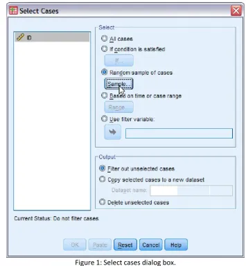
To select 10 subjects by simple random sampling, from menus choose Data → Select
Cases. You would be presented with this dialog box (Figure 1). Notice that there are two categories: Select and Output. At this moment, under Select, choose Random sample of cases option, and click Sample...
button. You would be presented with another dialog box namely Select Cases: Random Sample. There two options; by Approximately ___ % of all cases, or by Exactly ___ cases from the first ___ cases. We would be using Exactly ___ cases from the first ___ cases option and put in 10 in the first text box followed by 20 in the second text box. What it means is that we are selecting 10 subjects out of first 20 subjects in our list by simple random sampling. Since we only have 20 subjects in our list, it means that we are selecting all of them, and all of them possibly have a chance to be included in our sample of 10 subjects. The first option is self explanatory as we cannot specify exact number of subjects that we want included as the sampling frame gets larger and larger. Click Continue and we are back in Select Cases dialog box.
Notice that under Output category, there are three options. The first one by default is Filter out unselected cases. What it does it creates a new variable namely filter_$, and designate a value 1 for selected subjects/cases and 0 for unselected cases. This variable is a filter variable that denotes the status of selection of cases by SPSS in term of analysis. In Data View also we notice that the unselected cases are crossed out. By selecting the second option (Copy selected cases to a new dataset), it creates a new dataset with a specified name consisting only the selected cases. Let say we name the new dataset as simple_random_selected (please observe the naming style for SPSS), we would get a new dataset window opened consisting only selected 10 subjects.
Education in Medicine Journal
2012, VOL 4 ISSUE 1
DOI:10.5959/eimj.v4i1.4
you accidentally save over the original dataset after using this option.
For this step under Output, choose Copy selected cases to a new dataset. Save the newly generated dataset as simple_random_selected.sav.
Systematic random sampling
As mentioned before, systematic random sampling is just a matter of selecting a random number as starting point within the limit of a selected interval. Let say we require 10 subjects out of a list of 30 subjects, divide total number of subjects in sampling frame (30) by number sample size (10). We obtain an interval of 3 as a result (30/10=3). We would like to select a random number between 1 to 3 as a starting point in a list of 30 subjects. Start with a new empty dataset. Since we only need to generate one number only as a random starting point, in Data View just click on the first row first column of the empty dataset and key in any number, for example 0.
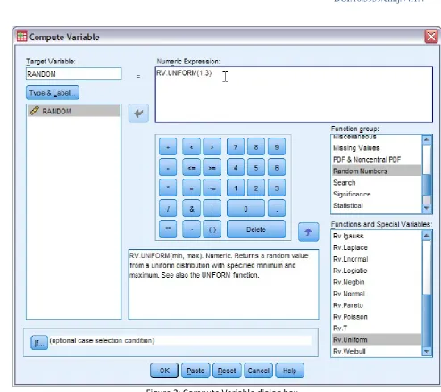
A new variable namely VAR00001 with only one case is generated. Go to Variable View and rename the variable to RANDOM. Under menus, choose Transform → Compute
Variable. You would be presented with this dialog box (Figure 2). In target variable, enter the name of our variable RANDOM. Under Function group select Random Numbers, followed by double clicking on Rv.Uniform under Functions and Special Variables. This step would automatically put Rv.Uniform function in Numeric expression text area in form of RV.UNIFORM(?,?). This function is described as RV.UNIFORM(min,max) with min is the lowest value in the interval and max is the largest value in the interval. In our case, we would like to generate a random value between 1 to 3, so naturally our min is 1 and max is 3. Not so since the interval between 1 to 3 is only 2 (3 minus 1), so decision for min
and max is not straight forward. Next, the function would generate random values between 1 to 3 with decimals (for example 1.39, 2.85). When we round the generated values, a value between 1 to 1.49 is rounded to 1, 1.5 to 2.49 is rounded to 2, and 2.5 to 3 is rounded to 3. You can see clearly that the chance to get a value of 2 is higher since the interval is wider (50 percent of time we will obtain a value 2). In order to obtain a random value between 1 to 3, we need to generate a value between 0.5 to 3.5 so that the rounded value is not only within the range of 1 to 3, but also the chance to obtain any of the three values (1, 2, 3) is equal (0.5 to <1.5: 1, 1.5 to <2.5: 2, 2.5 to <3.5: 3).
Edit our function accordingly in Numeric expression as RV.UNIFORM(0.5,3.5). Highlight the edited function, then again under Function group select Arithmetic, followed by double clicking on Rnd(1)under Functions and Special Variables. We would end up having RND(RV.UNIFORM(0.5,3.5)) in Numeric Expression. RND(numexpr) by default would give a rounded value of numexpr in multiple of 1 (i.e no decimal). In our case, it gives rounded value for expression RV.UNIFORM(0.3,3.5). Click OK. Click OK again when SPSS asks to change existing variable. We would obtain a random value between 1 to 3 with this step in place of our previously entered value. Save the dataset as one_random_value.sav. At this step you can already use this value as a starting point on your printed list of subjects in the sampling frame.
Education in Medicine Journal
2012, VOL 4 ISSUE 1
DOI:10.5959/eimj.v4i1.4
→ New → Syntax and we would be presented
with a Syntax Editor. Write the following syntax in text area on the right hand side of the window:
NEW FILE.
INPUT PROGRAM. LOOP #i=1 TO 30.
COMPUTE ID=$CASENUM. END CASE.
END LOOP. END FILE.
END INPUT PROGRAM. EXECUTE.
You can change the number of cases required by changing editing the third line of the syntax (30 to other number). From Syntax Editor menus choose Run → All . A new dataset
would be generated complete with 30 cases and identification number. Change the number of decimal place for variable ID to 0. Save the dataset as systematic_random.sav. Next, we would like indicate which cases are selected based on systematic random process. For starter, generate a new variable namely SELECT to denote the status of selection of the cases (similar to filter_$ variable that we described previously). We would assign a value 1 for selected cases and a value of 0 for unselected cases under variable SELECT. Check back our random starting point in one_random_value.sav dataset.
For example, I obtained 2 as a random starting point. For case number 2, we would give a value of 1, followed by successive third case after case number 2 (as for interval of 3). As a result, we would have case number 2, 5, 8, 11 and so on until case number 29 given value of 1 for variable SELECT. To automate this process, from menus choose Transform
→ Compute Variable. Set a value of 0 to our
target variable SELECT in Numeric Expression. This step would assign a value of 0 to all cases in the dataset. Next, we would like to assign a value of 1 to selected cases based on our
random starting value and systematic sampling. Go back to Compute Variable and set SELECT to a value of 1. Next, click If... button on the lower left side of the dialog box and you would be presented with Compute Variable: If Cases dialog box. Choose If case statisfies condition followed by entering MOD($CASENUM,3)=2 in the text box. Click Continue, followed by OK in the subsequent dialog box. You might be wondering what the function did for us.
Function MOD(numexpr,modulus) is a modulus function which returns the remainder when numexpr is divided by modulus. In our case we set the function as MOD($CASENUM,3)=2. By dividing case number by 3, the function would return 0 for every multiple of 3. Since we want to start from case number 2 instead, we would like to select subjects whose modulus of their respective case number is 2. You can see the effect of the steps as the selected cases are assigned a value of 1 starting from case number 2 up to case number 29 with an interval of 3. In another example, if we set an interval of 5 starting from case number 3, set the function as MOD($CASENUM,5)=3.
Having selected our cases, from menus choose Data → Select Cases . Choose If condition is satisfied under Select category, and click on If... button for the option. In the subsequent dialog box namely Select Cases: If, double click on SELECT variable name on the left hand side of the dialog box to have it entered in the text area on the right hand side. In the text area edit to SELECT=1, meaning that based on variable SELECT, we would like to select only cases with designated value of 1.
Education in Medicine Journal
2012, VOL 4 ISSUE 1
DOI:10.5959/eimj.v4i1.4
Save the newly generated dataset as systematic_random_selected.sav.
Stratified random sampling
For stratified random sampling dataset, we have to create a dataset consisting of 20 subjects as our sampling frame. As usual to represent the subjects, we need a variable named as ID. We also need a new variable namely STRATA to indicate the group or strata of the subjects. For this purpose, reopen our dataset simple_random.sav. As we already have 20 subjects complete with their identification number (variable ID), we just have to create a new variable STRATA. We would like to have 2 groups/strata for the subjects, let say group 1 and 2. For the first 10 subjects, set the value of variable STRATA as 1, with the remaining 10 subjects as 2. Save the modified dataset as stratified_random.sav.
Next, we need to split the dataset into different datasets for each of the group. As we have two groups in our dataset, we need to split it into two datasets. From menus choose Data → Select Cases . In the dialog
box, choose If condition is satisfied, followed by If... button to open Select Cases: If dialog box. In the text box, since we would like to choose first group (strata 1), enter STRATA=1. For the Output, choose Copy selected cases to a new dataset and set the dataset name as stratified_random_gr1. Save the new dataset as stratified_random_gr1.sav. Repeat the same steps by changing STRATA=1 to STRATA=2 in Select Cases: If dialog box and setting the new dataset name as stratified_random_gr2. Save the new dataset as stratified_random_gr2.sav.
From now on, respected readers may have noticed that the next step is straight forward. Since we have two separate datasets which represent sampling frame by strata, just do simple random sampling from each of the
strata. For example, we would like to select 10 subjects out of 20 subjects in sampling from. We would like to sample proportionately to the size of strata. Since each of the strata represents 50% of the sampling frame, we would like to randomly sample five subjects out of each strata (50% of strata size of 10 subjects). For each dataset, do simple random sampling to select five subjects. Save the datasets accordingly, for example str_rnd_gr1_sel.sav and str_rnd_gr2_sel.sav. Later you may combine the selected subjects back into a new dataset. To combine datasets, from menus choose Data → Merge File →
Add Cases, from which you can combine your currently active dataset with other currently opened dataset or other dataset. In our case, with dataset namely str_rnd_gr1_sel.sav opened, choose the mentioned menus and select str_rnd_gr2_sel.sav and just click OK in the subsequent dialog box.
You may try the whole steps mentioned in this section with dataset systematic_random.sav consisting of 30 subjects for sampling frame. Create a new variable namely STRATA (or just rename variable SELECT to STRATA) and set the first 20 subjects in group 1 and the remainders in group 2. We would like to sample 15 subjects in total and have the sampling proportionate to strata. Select one third of the sample (five subjects) from strata 2 and two third of the sample (10 subjects) from strata 1.
Cluster and multistage sampling
Education in Medicine Journal
2012, VOL 4 ISSUE 1
DOI:10.5959/eimj.v4i1.4
that we described before, the steps that we already discussed are also applicable here.
Random Allocation
In this section, I would demonstrate the steps for simple random allocation, block random allocation and stratified random allocation.
Simple random allocation
For starter, let say we have a sample of 20 subjects (use simple_random.sav) and we would like to divide the subjects into two groups: experimental (1) and control (2). We would generate a variable namely GROUP containing random values between 0.5 to 2.5, for which the rounded values would be 1 and 2. A value of 1 indicates case assignment to experimental group while a value of 2 indicates case assignment to control group. Recall our steps in systematic random sampling section as the steps are basically similar. From menus choose Transform --> Compute Variable, followed by setting Target Variable as GROUP. Under Numeric Expression key in RND(RV.UNIFORM(0.5,2.5)). Save as simple_random_allocation.sav. Take a look at variable GROUP values and count how many 1s and 2s that it has. Note how unequal the allocation by this method (or you might be lucky enough to obtain equally sized group). In my case I obtained 9 subjects in experimental group while the rest of 11 subjects in control group.
Next, let say we have a sample of 30 subjects (use systematic_random.sav) and we would like to allocate the subjects into three groups: experimental (1), generic (2) and placebo (3). We would generate a variable namely GROUP containing random values between 0.5 to 3.5, for which the rounded values would be 1, 2 and 3. A value of 1 indicates case assignment to experimental group, a value of 2 indicates case assignment to generic group, and a value of 3 indicates case assignment to 3. The steps
similar to the allocation for two groups described before. The only difference is only for our setting of Numeric Expression. Change it to RND(RV.UNIFORM(0.5,3.5)). Save as simple_random_allocation_3gr.sav. This time being I was lucky enough to obtain equally sized group.
For unequal group, let say we have a sample of 30 subjects (again use systematic_random.sav) and we would like to have them randomly allocated into experimental (1) and control (2) group, with control group to have twice as much subjects as experimental group. We would like to select 10 experimental subjects and 20 control subjects. We already know the steps for allocation into three groups as described before and it is still applicable here since after we obtaning the dataset with three grouping indicator (1, 2 and 3), just recode the value 2 and 3 to a value of 2. From menus choose Transform --> Recode into Same Variables. In the resulting dialog box, move variable GROUP into Numeric Variable box. In the same dialog box, click on Old and New Values, opening Recode into Same Variables: Old and New Values dialog box. To recode 2 and 3 to a value of 2 (representing control group), select Range option, enter 2 through 3, followed by 2 in New Value text box, then click on Add button. Click on Continue button, followed by OK button. Most likely we would obtain more '2's than '1's, so we obtained approximately the ratio of 2 to 1 for control to experimental group. Save as simple_random_allocation_unequal.sav.
Block random allocation
Education in Medicine Journal
2012, VOL 4 ISSUE 1
DOI:10.5959/eimj.v4i1.4
control group size twice as large as experimental group). By using simple random allocation, we may or may not get the group size that we want to obtain, so when control over group size is important, blocked allocation is suitable.
There are few things that we have to be clear before proceeding with block random allocation with equal group. Firstly, the block size (b) should be divisible of number of group (g). Let say, we would like to allocate the sample into group A and B (2 groups), possible block size is b = 2, 4, 6, ... n x g. Secondly, overall sample size should be divisible by block size. For example a sample size of 20 is divisible by block of 4 with no remainder (20/4=5, no decimal). Thirdly, number of blocks in a sample list is equal to sample size divided by block size, for example by setting a block size of 4, we would obtain 5 blocks of that size with a sample size of 20. Fourthly, determination of the number of possible combination of group order in a particular block size. When the block size is not equal to number of group, the number of possible combination of group order in a block is given by bCg = b! / g!(b-g)!. For example the number
possible combination when we have 2 groups (A, B) with block size of 4 is 6 (4! / 2!(4-2)! = 4.3.2.1 / 2.1.2.1 = 12/2 = 6). Thus we would have AABB, BBAA, ABAB, ABBA, BABA, and BAAB. When the block size is equal to number of group, the number of possible combination is given by g!. Thus when we have 3 groups (A, B, C) with block size of 3, the number of possible combination is 6 (3! = 3.2.1 = 6). Thus we would have ABC, ACB, BAC, BCA, CAB and CBA. You might find these rules useful to check the validity of your block random allocation.
To begin, let say we have a sample of 20 subjects (use dataset simple_random.sav). We would like to have them randomly allocated into experimental (1: A) and control (0: B) group, with each group consisting of five
Education in Medicine Journal
2012, VOL 4 ISSUE 1
DOI:10.5959/eimj.v4i1.4
values by block number. Next, from menus choose Transform --> Recode into Different Variables. In the resulting dialog box, move RRANDOM into Numeric Variable -> Output Variable box, then type in GROUP in Name text box under Output Variable, followed by clicking on Change button.
In the same dialog box, click on Old and New Values, opening Recode into Different Variables: Old and New Values dialog box. Recode 1 and 2 to a value of 1 (representing group A/experimental), and 3 and 4 to a value of 0 (representing group B/control). In Range, LOWEST through value option text box, enter 2, followed by 1 in New Value text box, then click on Add button. Similarly, type in 3 in Range, value through HIGHEST text box followed by 0 in New Value text box, then Add the recoding. Click on Continue button, followed by OK button. Note that in our resulting variable GROUP, the assignment is already done by block with this step. To make the assignment clearer, give value label to 0 and 1 for GROUP variable.
Edit accordingly under Variable View under Values column for variable GROUP (1 labelled as A and 0 labelled as B). In Data View, from menus choose View --> Value Labels to view our combination of As and Bs. Save as block_random_allocation.sav.
For another example, let say we have a sample of 15 subjects. We would like to have them randomly allocated into experimental (1: A) and control (0: B) group, with control group to have twice as much subjects as experimental group (unequally sized group). We would like to select five experimental subjects and 10 control subjects. Use dataset systematic_random.sav and randomly select 15 subjects based on simple random sampling for the purpose of this example. You may remove variable SELECT from the dataset. Save the dataset as simple_random_15.sav. We choose a block size of 3, two groups with
group A twice as large as group B. As the steps are basically similar to equal group, I would only describe the steps in details when necessary. Create variable BLOCK_NUM and assign block number to every successive 3 cases per block with RND($CASENUM/3 + 0.49) numeric expression. Next create variable RANDOM containing random values between 0 to 1.
Further, rank the random values by BLOCK_NUM. Recode the ranking values into two As (1) and B (0) by taking the lower two third of the ranking (rank 1 and 2) to group A and upper one third of the ranking (rank 3) to group B, and save into output variable GROUP. Label accordingly and then save as block_random_allocation_unequal.sav.
To demostrate the situation where we have three groups, use again the dataset systematic_random.sav. In this dataset, we have 30 subjects and we would like to allocate them equally into three groups namely experimental (1: A), generic (2: B) and placebo (0: C), so that we would have 10 subjects per group. We choose block size of 6, three groups with equal size. The basic combination for the assignment is AABBCC. For starter, create variable BLOCK_NUM and assign block number to every successive 6 cases per block with RND($CASENUM/6 + 0.49) numeric expression.
Education in Medicine Journal
2012, VOL 4 ISSUE 1
DOI:10.5959/eimj.v4i1.4
Pseudo-block random allocation
Using SPSS, we can imitate the characteristic of typical block random allocation (i.e. being able to control group size) by utilizing SPSS ability to select only specified number of subjects required. Recall how we did simple random sampling using Random sample of cases option by specifying a specific number of required subjects as the same option is also applicable here. For example, let say we have a sample of 10 subjects (use datasetsimple_random_selected.sav). We would like to have them randomly allocated into experimental and control group, with each group consisting of five subjects (equally sized group). With dataset simple_random_selected.sav opened, from menus choose Data → Select Cases . Under Select category, choose Random sample of cases option.
Using Exactly ___ cases from the first ___ cases option, choose 5 out of 10 subjects. Next, under Output category, use Filter out unselected cases option. As described in previous section, these steps would create a new variable namely filter_$ and cross out unselected case. To remove the crossing out of unselected cases, go back to Data → Select
Cases and select All cases under Select category. Notice that under variable filter_$ column, we would see 1 and 0 with 1 for selected cases and 0 for unselected cases. Using this attribute to our advantage, think of 1 as experimental group while 0 as control group. Rename variable filter_$ to GROUP. With that we already randomly allocated our sample into two groups. Save the dataset as pblock_random_allocation.sav.
For another example, let say we have a sample of 15 subjects. We would like to have them randomly allocated into experimental and control group, with control group to have twice as much subjects as experimental group (unqually sized group). We would like to
select five experimental subjects and 10 control subjects.
Use dataset systematic_random.sav and randomly select 15 subjects based on simple random sampling for the purpose of this example. You may remove variable SELECT from the dataset. Save the dataset as simple_random_15.sav. The steps are mainly similar to the steps for equally sized group. The only change that we need is to adjust Exactly ___ cases from the first ___ cases option by choosing 5 out of 15 subjects. With that we would obtain variable filter_$ with five of the values set to 1 while the remaining 10 subjects set to 0. After renaming variable filter_$ to GROUP, save the dataset as pblock_random_allocation_unequal.sav.
To demonstrate the situation where we have three groups, use dataset simple_random_15.sav. In this dataset, we have 15 subjects. We would like to allocate them equally into three groups (experimental, generic and placebo), so that we would have five subjects per group. We would like to first randomly allocate five subjects into experimental group, followed by allocating five more subjects into generic group. The remaining five subjects would be allocated into placebo group. From menus choose Data
→ Select Cases. Under Select category,
Education in Medicine Journal
2012, VOL 4 ISSUE 1
DOI:10.5959/eimj.v4i1.4
resulting variable filter_$ to GEN to denote the group allocation in generic group. A value of 1 is for being in generic group while a value of 0 is for being in other group. Go back to Select Cases dialog box to select All cases option to remove the crossing out of unselected cases. As the dataset started to materialize, from menus choose Transform --> Compute Variable. In the opened dialog box, type GROUP in Target Variable text box. In Numeric Expression text box, just set the value to 0 and click OK. Following this step, you would have a new variable namely GROUP. For this variable, we would assign a value of 0 to control group, 1 to experimental group and 2 to generic group. In other words, we would assign a value of 1 for cases whose status is 1 for variable EXP, a value of 2 for cases whose status is 1 for variable GEN, while no change is needed for control since the value for variable GROUP is already 0. To automate the assignment for experimental group, from menus choose Transform --> Compute Variable, followed by changing Numeric Expression to 1. Next, click If... button on the lower left side of the dialog box and you would be presented with Compute Variable: If Cases dialog box. Choose If case statisfies condition followed by entering EXP=1 in the text box. Click Continue, followed by OK in the subsequent dialog box. Click OK to change existing variable. Repeat the same steps for generic group by setting Numeric Expression to 2 and GEN=1 for If case statisfies condition text box. You would end up with four variable in the dataset: ID, EXP, GEN and GROUP. Since we already transferred the status of group allocation to variable GROUP, you may delete variables
EXP and GEN. Save as
block_random_allocation_3gr.sav.
Personally speaking, the steps for more than two groups in this section using Exactly ___ cases from the first ___ cases option is less ideal. Note that after our first selection of experimental cases, the chance of being
selected to experimental group among the remaining cases is no longer there, while at the same time also the chance of those assigned to experimental group to be selected in either generic or control group is nil. In short, the chance of being assigned to any of the three groups for all 15 subjects is no longer equal once assignment for experimental group is finished. Having said that, since blocking method itself reduces the randomness of assignment, in my opinion the steps might be applicable given right justifications.
Stratified random allocation
Stratified random allocation can be done easily with combination of the steps for stratified random sampling and simple random allocation described before. Simply put, split the dataset into few separate datasets by groups/strata. Next, for each resulting dataset, do simple random allocation. Lastly, combine the datasets into one final dataset consisting of mainly identification variable, strata variable and grouping/allocation variable. To demonstrate these steps, remember that we already did the first few steps up to when we generated
two datasets namely stratified_random_gr1.sav and
stratified_random_gr2.sav under stratified random sampling section. Assuming that the subjects in each strata are sample instead of sampling frame, for each dataset allocate the subjects into two groups following the basic steps of random allocation.
Education in Medicine Journal
2012, VOL 4 ISSUE 1
DOI:10.5959/eimj.v4i1.4
Conclusion
Random sampling and allocation could be accomplished using SPSS without the need for additional software. In this article, I laid out the steps for the processes in detail for each section together with clinically oriented examples. I would like to stress again the ability to link directly the data sets with the
random sampling and randomization processes is advantageous by sticking to SPSS. In writing the steps, I attempted to be as detail as possible so that respected readers would be able to follow closely the steps. It is hoped that this article would be a useful guide to researchers in sampling and allocating patients for their research using SPSS.
Education in Medicine Journal
2012, VOL 4 ISSUE 1
DOI:10.5959/eimj.v4i1.4
2012 VOL 4 ISSUE 1
DOI: 10.5959/eimj.4.1.2012.er1
Reference1.Bland M. Directory of randomisation software and services. 2011 [April 1, 2012];
Available from: http://www.users.york.ac.uk/~mb55/guide/ra
ndsery.htm.
2.Everitt B, Skrondal A. The Cambridge dictionary of statistics. 4th ed. New York: Cambridge University Press; 2010.
3.Trochim WMK. Research methods knowledge base. 2006 [March 27, 2012];
Available from: http://www.socialresearchmethods.net.
4.Daniel WW. Biostatistics: A foundation for analysis in the health sciences. 6th ed. USA: John Wiley & Sons; 1995.
5.Bland M. An introduction to medical statistics. 3rd ed. New York: Oxford University Press; 2000.
6.Schulz KF, Grimes DA. Generation of allocation sequences in randomised trials: chance, not choice. The Lancet. 2002;359(9305):515-9.
7.Altman DG, Bland JM. How to randomise. British Medical Journal. 1999;319(7211):703-4.
Further Reading
1.Alferes VR. Random assignment of units to experimental treatments.SPS. In: Levesque R, editor. Raynald's SPSS Tools. 2011. [December 12, 2011]; Available from: http://www.spsstools.net/Syntax/BlockDesign
/RandomAssignmentOfUnitsToExpTreatments .txt.