Robust Parameter Estimation for Fixed Effect Panel Data
Model in the Presence of Heteroscedasticity and High Leverage
Points
Muhammad Sani ∗1,3, Habshah Midi1,2, and Jayanthi Arasan2
1Institute for Mathematical Research, Universiti Putra Malaysia Serdang, Malaysia 2Department of Mathematics, Faculty of Science, UPM Serdang, Malaysia 3Department of Mathematical Sciences and IT, Federal University Dutsinma, Katsina
State, Nigeria
∗Corresponding author: [email protected]
In the presence of unknown heteroscedasticity structure and anomalous observations such as High Leverage Points (HLPs), the variance-covariance matrix of the ordinary least squares (OLS) estimator become bias and inconsistent in linear as well as in fixed effect (FE) panel data model. As a remedial measure, we propose Robust Heteroscedasticity Consistent Covariance Matrix (RHCCM) estimator based on Weighted Least Square in panel data model. In the proposed methods, weights are determined from HLPs detection methods so that the effect of HLPs can be minimized by assigning lower weights to HLPs. The numerical examples and simulation results indicate that the proposed RHCCM based on Fast Modified generalized Residuals (FMGt) offers substantial improvement over some existing estimators.
Keywords: HCCM, heteroscedasticity, high leverage point, Ordinary least squares, weighted least squares.
I.
Introduction
Fixed effect (FE) panel data model is used when the individual specific effect (unobserved time invariant effects) is correlated with the explanatory variables (V´ıˇsek, 2015). The or-dinary least squares (OLS) method is used to estimate the parameters of the model after the data transformation by mean centering (de-meaned transformation). However, the OLS can strongly be biased and inconsistent in the presence of high leverage points (HLPs) and heteroscedasticity (unequal variances of the er-rors). HLPs referred to observations that are far away from the majority of the data points in X-direction. Many researches are avail-able regarding outlying observations problem in FE panel data regression model, such as (Bakar and Midi, 2015, Bramati and Croux, 2007, Maronna et al., 2006, Verardi and
Wag-ner, 2011). Their methods only addressed the problem of outliers but the combined problem of outliers particularly HLPs and heteroscedas-ticity in FE model is still missing in the litera-ture.
by White (1980) is used to remedy the prob-lem heteroscedasticity of unknown form. There are many versions of HC0 estimator proposed by MacKinnon and White (1985), Cribari-Neto (2004) and Cribari-Neto et al. (2007) denoted by HC1, HC3, HC4 and HC5 respectively. Similarly, when heteroscedasticity comes along with the presence of HLPs in the data set, the HCCM estimator is bias which tends to per-form poorly by providing unreliable parameter estimates.
The estimation strategy used for a model with heteroscedasticity of unknown form in the pres-ence of HLPs as suggested by Furno (1996) is to perform ordinary least squares (OLS) esti-mation, and then employed a robust HCCM estimator which used residuals from weighted least squares (WLS) instead of OLS. The short-coming of this method is that, the weighting method (hat matrix) used is inefficient as it suf-fers from masking and swamping effect (Hab-shah et al., 2009). This motivated us to pro-pose weighting methods which are more effi-cient than hat matrix, in order to remedy the effects of HLPs and heteroscedasticity in FE panel data model.
In this study three robust weighting methods based on HLPs detection measures were used for robust HCCM estimator in FE panel data regression model. In this article, a more effi-cient robust weighting technique is used in or-der to successfully down weight the HLPs in a data set. The weights are based on; Robust ma-halanobis distance based on minimum volume ellipsoid (RMD(MVE)), Diagnostic robust gen-eralized potential based on index set equality (DRGP(ISE)) and proposed fast modified gen-eralized studentized residuals (FMGt). Simi-larly, MM-centering method for data transfor-mation will be employed to reduce the effects of HLPs.
Section 2 introduced the least weighted Square (LWS) estimation method. Section 3 explained classical HCCM and robust HCCM estimator. Section 4 described the propose robust estima-tion methods. The simulation study is pre-sented in Section 5 and the real data examples
are given in Section 6. Section 7 presents the conclusion.
II.
Least Weighted Squares
(LWS) Estimator
V´ıˇsek (2015) proposed an estimation technique for the fixed effect (FE) panel data model termed least weighted squares (LWS). Consider a FE model as,
yit = αi+ x0itβ+ eit (1)
where, i = 1,2, . . . , n, t = 1,2, . . . , T, yit
are the response variables, xit is the kth
ex-planatory variables,αi is the unobserved
time-invariant effects andeitis the error term that is
assumed to be normal, uncorrelated across in-dividual units and time. Also,cov(xit, αi)6= 0
and αi is usually eliminated when the data
is transformed by demeaned transformation within each time series by mean given as:
(yit−yi.) = (xit−xi.)β+eit (2)
where, yi. = T1 PT
t=1yit, xi.= T1 PTt=1xit and
Equation (2) becomes;
˜
yit= ˜xitβ+eit (3)
where, ˜yit=yit− yi.and ˜xit=xit− xi.The
least weighted squares (LWS) estimator pro-posed by V´ıˇsek (2015) is obtained by first com-puting the residual of the (i,t)thobservations from Equation (1) as:
rit= yit−x0itβ.
By denoting the qth squared residuals order statistic byr2(q)(β), where q = 1,2,. . . ,nT so that,
r2(1)(β)≤r(2)2 (β)≤ · · · ≤r2(n T)(β),
followed by minimizing the weighted sum of squares residuals as,
W SS(β,−→w) =
nT
X
q=1
where, weight (wq) is defined aswq ∈[0, 1] for
q = 1,2,. . . , nT for more details see (V´ıˇsek, 2015). The LWS estimator is given as:
b
β(LW S) = argmin
β nT
X
q=1
wq r2q(β)
= (X0W X)−1X0W y
where, W is a diagonal matrix of wq. The
ab-solute residuals (r(it)(β)0s) value distribution
function denoted byFβn(r), its derivation shows that βb(LW S) is among the solutions of the
normal equations, see V´ıˇsek (2011)
n
X
i=1
T
X
t=1
w FβnT(|rit(β)|)
xit(yit−x˜itβ) = 0
It has been proven that βb(LW S) is consistent
under certain assumptions.
III.
HCCM and Robust
HCCM Estimators
White (1980) proposed the heteroscedasticity consistent covariance matrix (HCCM) estima-tor known as HC0 where he replaced σq2 with
b
e2q in the covariance matrix of βbas:
HC0 = (x0x)−1x0Φˆ0x(x0x) −1
(4)
where, ˆΦ0= diagbe
2
q}. Different adjustment of
HC0 was done by many researchers which give rise to HC1, HC2 and HC3. They are generally biased for small sample sizes, see (Furno, 1996, Hausman and Palmer, 2012, Lima et al., 2009). This research will only focus on HC4 and HC5. The HC4 proposed by Cribari-Neto (2004) was build under HC3, which is defined as follows:
HC4 = (x0x)−1x0Φˆ4x(x0x) −1
(5)
where, ˆΦ4= diag
n
b
e2
q (1−hq)δq
o
forq= 1, . . . , nT
with δq= min
n
4, hq
h
o
, which control the dis-count factor of theqth squared residuals, given by the ratio of hq and the average of hq’s (h).
Since 0 < 1−hq < 1 and δq > 0 it implies
that 0 < (1−hq)δq < 1. The larger hq is
rel-ative to h, the more the HC4 discount factor inflates the qth squared residual. The trunca-tion at 4 amounts to twice what is used in the definition of HC3; that is, δq= 4 when hq >
4h = 4p/nT. The result obtained by Cribari-Neto (2004) suggested HC4 inference in finite sample size relative to HC3.
Similarly, another modification of the exponent (1−hq) of HC4 was proposed by Cribari-Neto
et al. (2007) to control the level of maximal leverage. The estimator is termed HC5, defined as:
HC5 = (x0x)−1x0Φˆ5x(x0x) −1
(6)
where the value of ˆΦ5= diag
b
e2
q
√
(1−hq)αq
for q = 1, . . . , nT with the quantity
αq= min
n h
q
h, max
4, khmax
h
o
, which deter-mine the amount of increased of theqthsquared residual, given by the ratio between hmax
(max-imal leverage) and h (mean leverage value of hq’s). When hhq ≤4 it follows that αq = hhq.
Also, since 0 < 1−hq < 1 and αq > 0, it
implies that 0<(1−hq)αq <1 and k is a
con-stant ranges between 0 < k < 1 where HC5 reduces to HC4 when k = 0. K value was sug-gested to be chosen as 0.7 by Cribari-Neto et al. (2007) following his simulation result that leads to efficient quasi-t inference.
Furno (1996) suggested using weighted least squares (WLS) regression residuals instead of OLS residuals used by White (1980) in HC0 estimator. The weight is based on the hat ma-trix (hi) and the robust (weighted) version of
HC0 is defined as:
HC0W = (x0W x)
−1
x0WΦb0wW x(x0W x)
−1
(7) where, W is ann×ndiagonal matrix with,
wq= min (1, c/hq), (8)
and c is the cutoff point,c= 1nT.5p,pis the num-ber of parameters together with the intercept,
b
Φ0w= diag {ee
2
q}witheeqbeing the q
thresiduals
leveraged observations are weighted by (c/hq)
to reduce their intensity and wq is considered
as the weight, so that the WLS estimator of β
is,
e
β = (X0W X)−1X0W Y.
The robust HCCM estimators for the HC4 and HC5 based on Furno’s weighting method are
HC4W and HC5W define as:
HC4W = (x0W x)
−1
x0WΦb4wW x(x0W x)
−1
(9)
where, Φˆ4w= diag
e
e2
q
(1−h∗ q)
δ∗q
for
q = 1, . . . , nT withδq∗= minn4, h
∗ q
h∗
o
, andh∗qis the qth diagonal elements of the weighted hat
matrix Hw =
√
W x(x0W x)−1x0√W . And,
HC5W = (x0W x)
−1
x0WΦb5wW x(x0W x)
−1
(10)
where the values of ˆΦ5w= diag
(
e
e2
q q
(1−h∗ q)
α∗q
)
for q = 1, . . . , nT with the expo-nent α∗q= minn h
∗ q
h∗, max
4, kh∗max
h∗
o
. The Furno’s weighted least square method de-scribed here denoted by WLSF will be applied
to the transformed FE panel data model in Equation (3) and obtain an estimate which is based on Furno’s weighting method.
IV.
Proposed Robust HCCM
Estimators
The idea of Furno (1996) was employed to for-mulate new RHCCM estimator base on HLPs identification weighting method; Robust maha-lanobis distance based on minimum volume el-lipsoid (RMD(MVE)), diagnostic robust gen-eralized potential based on index set equal-ity (DRGP(ISE)) and fast modified generalized studentized residualsl (FMGt). These methods are more efficient than the hat matrix used by Furno for the identification of HLPs (Habshah et al., 2009). We also employed robust center-ing method (MM-centercenter-ing) for the data tran-formation instead of classical mean-centering used by V´ıˇsek (2015) in order to reduce the effect of HLPs.
MM-centering is a robust technique of data transformation proposed by Bakar and Midi (2015), the centering involves transformation of panel data within each time series. The usual mean centering is highly sensitive to HLPs (Bramati and Croux, 2007). As an alterna-tive, the centering using median is put forward. However, for uncontaminated data median cen-tering was found to have low efficiency than the mean and causes non linearity to the trans-formed data (Maronna et al., 2006). This af-fects the efficiency of robust estimators when there is no HLPs. The MM-centering method is introduced in order to bring back linearity into the transformed data and also to provide high efficiency.
The MM-estimate of location was originally proposed by Yohai (1987). The goal was to produce a high efficiency and high breakdown point estimator. The procedure is given by: Firstly, compute S-estimates of location and covariance to obtain the preliminary scale es-timate, ˆσn:
ˆ
σn= min t sn (t).
The scale estimate is obtained by minimizing an M-estimate of scale. Thus, the initial esti-mate has a high breakdown point of 50% and it is also equivariance. The location S-estimate ˆ
µnis defined by:
ˆ
µn= arg mintsn(t).
Tukey’s Bisquare weight function was em-ployed to down weight HLPs, where ρ is given as:
ρ(x) =
1
6c4x6− 21c2x4+ 12x2, if |x| ≤c c2
6, if |x|> c
centering. The demeaned transformed data within each time series by MM centering is now given as:
yit−µˆmm{yit}=
x(itk)−µˆmm
n
x(itk)
o
β+eit
(11) for 1 ≤ t ≤ T, 1 ≤ i ≤ n, and 1 ≤ k ≤ K, where x(k) is the kth explanatory variables.
A. Robust HCCM Estimator based
on RMD(MVE)
Mahalanobis (1936) introduced a diagnos-tic measure of the deviation of an observa-tion from its center named Mahalanobis Dis-tance (MD), in which the independent vari-ables of the qth observations are presented
as xq = (1, xq1, xq2, . . . , xqk) = (1, Rq) so
that Rq = (xq1, xq2, . . . , xqk) will be k
-dimensional row vector, where the mean and covariance matrix vector are R = nT1 PnT
q=1Rq
and CV = nT1−1PnT
q=1 Rq−R
0
(Rq −R)
re-spectively. The MD for the qth points is given as:
M Dq =
r
Rq−R)
0
(CV)−1(Rq−R
(12)
where, q = 1, 2, . . . , nT. The average vector
R and covariance matrixCV in Equation (12) are not robust and easily affected by HLPs. Rousseeuw (1984) recommended using Robust Mahalanobis Distance (RMD) as in Equation (12) with slight modification where the R and
CV are obtained from minimum volume el-lipsoid (MVE). The corresponding CV is pro-vided by the ellipsoid and multiplied by a suit-able factor in order to obtain consistency. We suggest the cut off value of RMD as in Equation (13).
cd= median (RM Dq)+3.MAD(RM Dq) (13)
where, MAD stands for median absolute deviation. The weight obtained by this RMD(MVE) method is given by:
wqr= min (1, cd/RM Dq), (14)
so that HLPs are weighted by (cd/RM Dq) and
non leverage by 1. To obtain the RHCCM esti-mator based on RMD(MVE) weighting method denoted by WLSRM D, we replace Equation (8)
by (14) and follow Furno’s robust HCCM esti-mation method as discussed in Section (4.1).
B. Robust HCCM Estimator based
on DRGP(ISE)
Lim and Midi (2016) proposed diagnostic ro-bust generalized potential (DRGP) based on index set equality (ISE) in order to reduce the effect of swamping/masking and computional complexity of DRGP based on minimum vol-ume ellipsoid (MVE). The ISE was developed from the fast minimum covariance determinant (MCD). ISE was tested and found to execute highly faster in the estimation of robust esti-mator of scale and location. Thus, ISE has faster running time compared to MVE (Lim and Midi, 2016). The DRGP(ISE) consist of two steps whereby RMD based on ISE is utilised to detect the suspected HLPs.
The generalized potential (ˆpq) is employed on
the second step to check all the suspected iden-tified HLPs, those possess a low leverage point will be put back to the ‘R’ group. This tech-nique continued until all points of the ‘D’ group has been checked to confirm whether they can be referred as HLPs. The DRGP(ISE) denoted asDRGPq is defined as follows:
DRGPq =
h(−q D) f or q∈D h(q−D)
1−h(q−D)
f or q ∈R
(15) The cut-off point for DRGPq is given by:
CDRGPq=median(DRGPq) + 3QnT (DRGPq)
(16) where QnT=c{|xq−xj |;< j}(k) is a pair wise
order statistic for all distance proposed by Rousseeuw and Van Zomeren (1990) wherek=
h
.C2 ≈ h.C2/4 and h = [nT /2] + 1. They
make used of c = 2.2219, as this value will provide QnT a consistent estimator for
exceed CDRGPq then, the case with the least
DRGPqwill return to the estimation subset for
re-computation of DRGPq. The values of
di-agnostic robust generalized potential (DRGP) based on final ‘D’ set is the DRGP(ISE) rep-resented by DRGPq and the ‘D’ points will
be declared as HLPs. Now, the DRGP(ISE) weight can be obtained as follows:
wqd=min(1, CDRGPq/DRGPq) (17)
where, the HLPs are weighted by (CDRGPq/DRGPq) and non leverage by
1. We also replace Equation (8) by (17) and employed RHCCM estimation methods of Furno as discussed in Section (4.1) to obtain the RHCCM estimator based on DRGP(ISE) weighting method denoted by WLSDRGP.
C. Robust HCCM Estimator based
on FMGt
We suspect that the proposed RHCCM based on DRGP(ISE) weighting method will be af-fected by good HLPs because the RMD(ISE) only detect HLPs and unable to classify obser-vations into good and bad HLPs. Hence good observations will be given low weight and the efficiency of the RHCCM estimator tends to decrease as the number of good leverage points increases. As such we propose to firstly clas-sify observations into regular, good and bad HLPs, and vertical outliers, before formulating weighting method.
The proposed classification method is similar to Alguraibawi et al. (2015) with slight modi-fication whereby the modified generalized stu-dentized residual (MGtq) is established based on the Reweighted Least Squares (RLS) and DRGP(ISE) as initial estimates to make com-putation very fast compared to DRGP(MVE). Subsequently, theM Gtq is given by,
M Gtq =
b
eq(R∗)
b
σR∗−1√1−h∗∗
q(R∗)
, f or q ∈R∗
b
eq(R∗)
b
σ
R∗√1+h∗∗ q(R∗)
, f or q /∈R∗
(18) where beq(R∗),
b
σ(R∗) are the OLS residuals and
residuals standard error for remaining set R,
respectively, once theR∗ set is identified based on RLS and DRGP(ISE). The cut off point (CM Gtq) is calculated as follows:
CM Gtq=median(M Gtq) +cM AD(M Gtq)
(19) The classification of observations into the four categories is called fast modified generalized studentized residuals (FMGt). The classifica-tion scheme is as follows:
1. Regular observation (RO): An observation is declared as regular observation if ;
|M Gtq| ≤CM Gtq and |DRGP q| ≤CDRGP q
2. Vertical outlying observation (VO): An ob-servation is declared as VO if ;
|M Gtq|> CM Gtq and |DRGP q| ≤CDRGP q
3. Good leverage observation (GLO): An ob-servation is declared as GLO if ;
|M Gtq| ≤CM Gtq and |DRGP q|> CDRGP q
4. Bad leverage observation (BLO): An ob-servation is declared as BLO if ;
|M Gtq|> CM Gtq and |DRGP q|> CDRGP q
Once the bad HLPs and vertical outliers are identified, the weight is defined as:
wqr= min (1, CM Gtq/M Gtq), (20)
The RHCCM estimator based on FMGt weight denoted as WLSF M Gt is then
formu-lated by replacing Equation (8) by (20). It is important to note that the proposed WLSF M Gt
is expected to be more efficient because the weighting function is based only on VO and BLOs.
V.
Simulation Study
Monte Carlo simulation is used to evaluate the performances of proposed weighting method (WLSRM D,WLSDRGP,WLSF M Gt) in FE panel
N 0, σe2, αi ∼N(0, 5) and the vector of
co-efficients β equal to a vector of ones. Fol-lowing V´ıˇsek (2015) the independent variables (xit1, xit2, xit3) are generated from standard
normal distribution. Three sample sizes n = 5, 10, 15 with the corresponding t= 10, 15 20 were replicated twice to form n = 10, 20, 30 and t= 20, 30, 40 respectively, in order to cre-ate heteroscedasticity. The skedastic function is defined as σ2e = exp{c1xit1} (Lima et al.,
2009) where the value of c1 = 0.45 was
cho-sen such that λ ≈ 87.5 and will be constant among the sample sizes. The strength (de-gree) of heteroscedasticity is measured by λ= max σ2
e
/min(σ2
e) whereby, for
homoscedas-ticity λ= 1.
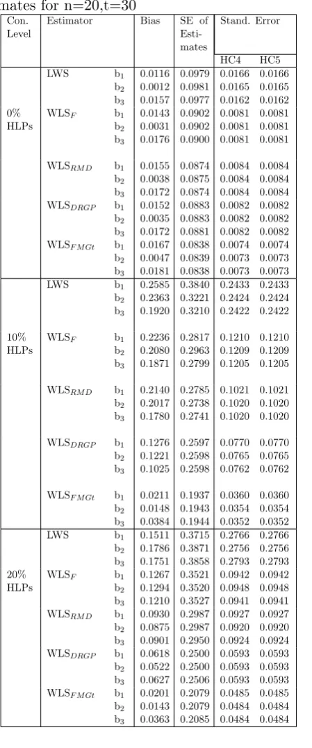
The data were contaminated by introducing high leverage points (HLPs) which are ran-domly generated from N(1,10), at 0%, 10% and 20% contamination level with R=1000 replications. The most efficient and best method is the one with lowest bias, lowest standard error of the estimate, lowest stan-dard error of HC4 and HC5. Results from Table (1) to (3) show the performance of the proposed methods (WLSRM D, WLSDRGP and
WLSF M Gt) and the existing methods (LWS
and WLSF), at different sample sizes and
HLPs contamination level. The results show that all the proposed methods were more effi-cient than the existing methods, by providing smaller bias, and standard error of HC4 and HC5. However, justification based on stan-dard error of the estimates here is improper and inefficient, as the structure of heteroscedas-ticity is unknown. Therefore, the estimation will be based on the HCCM estimator (HC4 and HC5). The results of these two methods are close to each other. The HC4 and HC5 based on WLSF M Gt was found to be the best
method due to the smaller value of bias, and standard error of HC4 and HC5. Figures 1-3 show the performance of all the methods at 20% HLPs contamination level with different sample sizes, where WLSF M Gt is the best
fol-lowed by WLSDRGP, WLSRM D, WLSF, and
fi-nally LWS.
Table 1: Simulation result of panel data esti-mates for n=10,t=20
Con. Level
Estimator Bias SE of Esti-mates
Stand. Error
HC4 HC5
LWS b1
b2 b3 0.0006 0.0021 0.0216 0.1476 0.1480 0.1460 0.0444 0.0468 0.0454 0.0444 0.0468 0.0454 0 % HLPs
WLSF b1
b2 b3 0.0024 0.0059 0.0234 0.1342 0.1344 0.1334 0.0185 0.0187 0.0184 0.0185 0.0187 0.0184 WLSRM D b1
b2 b3 0.0021 0.0064 0.0245 0.1305 0.1308 0.1297 0.0197 0.0203 0.0196 0.0197 0.0203 0.0196 WLSDRGP b1
b2 b3 0.0019 0.0062 0.0243 0.1317 0.1319 0.1309 0.0190 0.0194 0.0189 0.0190 0.0194 0.0189 WLSF M Gt b1
b2 b3 0.0044 0.0062 0.0241 0.1252 0.1255 0.1245 0.0174 0.0179 0.0174 0.0174 0.0179 0.0174
LWS b1
b2 b3 0.2832 0.3042 0.2437 0.3172 0.3095 0.3111 0.2323 0.2087 0.2297 0.2323 0.2087 0.2297 10% HLPs
WLSF b1
b2 b3 0.2284 0.2660 0.2310 0.2782 0.2738 0.2745 0.0841 0.0774 0.0755 0.0841 0.0774 0.0755
WLSRM D b1
b2 b3 0.2590 0.2999 0.2646 0.2733 0.2694 0.2690 0.0915 0.0855 0.0842 0.0915 0.0855 0.0842
WLSDRGP b1
b2 b3 0.1088 0.1523 0.1152 0.2709 0.2660 0.2668 0.0826 0.0756 0.0747 0.0826 0.0756 0.0747
WLSF M Gt b1
b2 b3 0.0025 0.0302 0.0285 0.2017 0.2180 0.2186 0.0478 0.0448 0.0453 0.0479 0.0448 0.0453
LWS b1
b2 b3 0.1941 0.1739 0.1830 0.3640 0.3559 0.3550 0.2395 0.2495 0.2549 0.2395 0.2495 0.2549 20% HLPs
WLSF b1
b2 b3 0.1023 0.1142 0.1351 0.3228 0.3231 0.3131 0.0860 0.0874 0.0879 0.0860 0.0874 0.0879 WLSRM D b1
b2 b3 0.1041 0.1213 0.1395 0.2901 0.2921 0.2927 0.0849 0.0861 0.0867 0.0849 0.0861 0.0867 WLSDRGP b1
b2 b3 0.0714 0.0755 0.0628 0.2720 0.2749 0.2556 0.0649 0.0667 0.0670 0.0649 0.0667 0.0670 WLSF M Gt b1
Table 2: Simulation result of panel data esti-mates for n=20,t=30
Con. Level
Estimator Bias SE of Esti-mates
Stand. Error
HC4 HC5
LWS b1
b2 b3 0.0116 0.0012 0.0157 0.0979 0.0981 0.0977 0.0166 0.0165 0.0162 0.0166 0.0165 0.0162 0% HLPs
WLSF b1
b2 b3 0.0143 0.0031 0.0176 0.0902 0.0902 0.0900 0.0081 0.0081 0.0081 0.0081 0.0081 0.0081
WLSRM D b1
b2 b3 0.0155 0.0038 0.0172 0.0874 0.0875 0.0874 0.0084 0.0084 0.0084 0.0084 0.0084 0.0084 WLSDRGP b1
b2 b3 0.0152 0.0035 0.0172 0.0883 0.0883 0.0881 0.0082 0.0082 0.0082 0.0082 0.0082 0.0082 WLSF M Gt b1
b2 b3 0.0167 0.0047 0.0181 0.0838 0.0839 0.0838 0.0074 0.0073 0.0073 0.0074 0.0073 0.0073
LWS b1
b2 b3 0.2585 0.2363 0.1920 0.3840 0.3221 0.3210 0.2433 0.2424 0.2422 0.2433 0.2424 0.2422 10% HLPs
WLSF b1
b2 b3 0.2236 0.2080 0.1871 0.2817 0.2963 0.2799 0.1210 0.1209 0.1205 0.1210 0.1209 0.1205
WLSRM D b1
b2 b3 0.2140 0.2017 0.1780 0.2785 0.2738 0.2741 0.1021 0.1020 0.1020 0.1021 0.1020 0.1020
WLSDRGP b1
b2 b3 0.1276 0.1221 0.1025 0.2597 0.2598 0.2598 0.0770 0.0765 0.0762 0.0770 0.0765 0.0762
WLSF M Gt b1
b2 b3 0.0211 0.0148 0.0384 0.1937 0.1943 0.1944 0.0360 0.0354 0.0352 0.0360 0.0354 0.0352
LWS b1
b2 b3 0.1511 0.1786 0.1751 0.3715 0.3871 0.3858 0.2766 0.2756 0.2793 0.2766 0.2756 0.2793 20% HLPs
WLSF b1
b2 b3 0.1267 0.1294 0.1210 0.3521 0.3520 0.3527 0.0942 0.0948 0.0941 0.0942 0.0948 0.0941 WLSRM D b1
b2 b3 0.0930 0.0875 0.0901 0.2987 0.2987 0.2950 0.0927 0.0920 0.0924 0.0927 0.0920 0.0924 WLSDRGP b1
b2 b3 0.0618 0.0522 0.0627 0.2500 0.2500 0.2506 0.0593 0.0593 0.0593 0.0593 0.0593 0.0593 WLSF M Gt b1
b2 b3 0.0201 0.0143 0.0363 0.2079 0.2079 0.2085 0.0485 0.0484 0.0484 0.0485 0.0484 0.0484
Table 3: Simulation result of panel data esti-mates for n=30,t=40
Con. Level
Estimator Bias SE of Esti-mates
Stand. Error
HC4 HC5
LWS b1
b2 b3 0.0063 0.0120 0.0015 0.0939 0.0937 0.0938 0.0126 0.0126 0.0127 0.0113 0.0113 0.0113 0% HLPs
WLSF b1
b2 b3 0.0045 0.0120 0.0021 0.0927 0.0926 0.0927 0.0107 0.0107 0.0107 0.0107 0.0107 0.0107
WLSRM D b1
b2 b3 0.0072 0.0146 0.0047 0.0922 0.0921 0.0922 0.0107 0.0107 0.0107 0.0107 0.0107 0.0107
WLSDRGP b1
b2 b3 0.0072 0.0146 0.0046 0.0923 0.0922 0.0923 0.0107 0.0101 0.0107 0.0107 0.0101 0.0107 WLSF M Gt b1
b2 b3 0.0071 0.0151 0.0143 0.0914 0.0913 0.0914 0.0105 0.0105 0.0105 0.0105 0.0105 0.0105
LWS b1
b2 b3 0.2976 0.3481 0.3741 0.3424 0.3423 0.3421 0.2318 0.2317 0.2325 0.2318 0.2317 0.2325 10% HLPs
WLSF b1
b2 b3 0.2686 0.2792 0.2908 0.2876 0.2819 0.2832 0.1582 0.1592 0.1608 0.1582 0.1592 0.1608
WLSRM D b1
b2 b3 0.2070 0.2202 0.2329 0.2685 0.2619 0.2634 0.1168 0.1170 0.1170 0.1168 0.1170 0.1170
WLSDRGP b1
b2 b3 0.1510 0.1645 0.1737 0.2125 0.2244 0.2451 0.0839 0.0856 0.0856 0.0839 0.0856 0.0856
WLSF M Gt b1
b2 b3 0.0330 0.0208 0.0283 0.1990 0.1986 0.1988 0.0420 0.0416 0.0425 0.0420 0.0416 0.0425
LWS b1
b2 b3 0.1855 0.2048 0.1908 0.3935 0.3984 0.3906 0.2324 0.2336 0.2331 0.2324 0.2336 0.2331 20% HLPs
WLSF b1
b2 b3 0.1082 0.1023 0.1064 0.2966 0.2979 0.2979 0.1179 0.1184 0.1182 0.1179 0.1184 0.1182
WLSRM D b1
b2 b3 0.0786 0.0783 0.0708 0.2732 0.2729 0.2833 0.8175 0.8180 0.8179 0.8175 0.8180 0.8179
WLSDRGP b1
b2 b3 0.0417 0.0423 0.0265 0.2330 0.2342 0.2343 0.5751 0.5804 0.5793 0.5751 0.5804 0.5793
WLSF M Gt b1
Figure 1: plot of HC5 SE for n=10,t=20
Figure 2: plot of HC5 SE for n=20,t=30
Figure 3: plot of HC5 SE for n=30,t=40
VI.
Numerical Examples
In this section, the proposed robust methods (WLSRM D, WLSDRGP and WLSF M Gt) and
the existing robust methods (LWS, WLSF) will
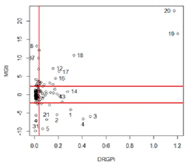
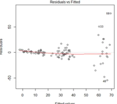
be applied to a real panel data set in order to evaluate their performances. Firstly, we con-sider a set of grunfeld investment data contain-ing 200 observations taken from Kleiber and Zeileis (2008). The data represent investment of 10 firms over 20 years (1935 – 1954), with investment as the response variable. Value of firms and value of the firm’s capital stock are treated as explanatory variables. This data set was diagnosed using FMGt with DRGP and found that it contains 46 outlying observations, where 19 of them are GLO, the remaining 27 are VO and BLO as shown in Figure 4. How-ever, there is a presence of heteroscedasticity in this data set due to the funnel shape produce by a plot in Figure 5.
Figure 4: plot of MGTi vs DRGPi for grunfeld data
Table 4 presents the result of proposed and existing methods in grunfeld investment data set. The result indicates that WLSF M Gt is the
Figure 5: plot of residuals vs fitted value for grunfeld data
Figure 6: plot of residuals vs fitted value for artificial data
The second example is an artificial panel data set, generated according to Bramati and Croux (2007) simulation method consisting 100 observations for 5 individuals observed over a period of 20 years. The response variable is generated according to Equation (1) with
eit ∼ N 0, σ2e
, αi ∼ U(0, 20) where σe2 =
exp{c1x1} with c1 = 0.65 (Lima et al., 2009).
The vector of coefficients β equal to a vector of ones. The three independent variables are generated from standard normal distribution. Figures 6 and 7 indicate the presence of
het-Table 4: Regression estimates for the grunfeld investment data set
Estimator Coeff. of Esti-mates
SE of Esti-mates
Stand. Error
HC4 HC5 LWS b1
b2
0.1027 0.1991
0.0153 0.0198
0.0005 0.0028
0.0005 0.0028 WLSF b1
b2
0.0908 0.2337
0.0142 0.0203
0.0003 0.0014
0.0003 0.0014 WLSRM D b1
b2
0.0993 0.2611
0.0132 0.0191
0.0004 0.0016
0.0004 0.0017
WLSDRGP b1
b2
0.0882 0.2198
0.0133 0.0182
0.0003 0.0009
0.0003 0.0009 WLSF M Gt b1
b2
0.0928 0.1970
0.0084 0.0131
0.0002 0.0005
0.0002 0.0006
Figure 7: plot of MGTi vs DRGPi for artificial data
eroscedasticity and outlying observations in the data respectively.
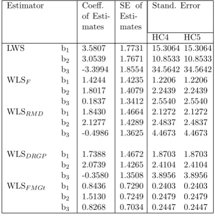
Table 5 presents the result of artificial panel data set. The result indicates that the pro-posed method (WLSF M Gt) is the best and most
efficient method as it gives the lowest stan-dard error of HC4 and HC5, lowest stanstan-dard error of the estimates, followed by WLSDRGP,
Table 5: Regression estimates for the artificial panel data set
Estimator Coeff. of Esti-mates
SE of Esti-mates
Stand. Error
HC4 HC5 LWS b1
b2
b3
3.5807 3.0539 -3.3994
1.7731 1.7671 1.8554
15.3064 10.8533 34.5642
15.3064 10.8533 34.5642 WLSF b1
b2
b3
1.4244 1.8017 0.1837
1.4235 1.4079 1.3412
1.2206 2.2439 2.5540
1.2206 2.2439 2.5540 WLSRM D b1
b2
b3
1.8430 2.1277 -0.4986
1.4664 1.4289 1.3625
2.1272 2.4837 4.4673
2.1272 2.4837 4.4673
WLSDRGP b1
b2
b3
1.7388 2.0739 -0.3580
1.4672 1.4265 1.3508
1.8703 2.4104 3.8956
1.8703 2.4104 3.8956 WLSF M Gt b1
b2
b3
0.8436 1.5130 0.8268
0.7290 0.7249 0.7034
0.2403 0.2479 0.2447
0.2403 0.2479 0.2447
VII.
Conclusion
The main focus of this study is to develop a reliable estimation method for FE panel data model for rectifying the problem of het-eroscedasticity in the presence of HLPs. The performance of the LWS estimator is very poor. The RHCCM based on hat matrix weight-ing method, i.e W LSF also not very efficient
as it suffers from swamping and masking ef-fect. In this study, we propose robust estima-tion methods in FE panel data model which employ residuals from weighted least squares (WLS) based on high leverage points detection measure (RMD, DRGP and FMGt) weighting methods in computing robust heteroscedastic-ity consistent covariance matrix (RHCCM) es-timator. The results based on both simulation and numerical examples signify that the pro-posed RHCCM estimator based on FMGT out-performed the existing methods (LWS,W LSF)
and other proposed methods by providing the least bias and least standard errors of HC4 and HC5.
References
[1] Alguraibawi, M., Midi, H., and Imon, A. (2015). A new robust diagnostic plot for classifying good and bad high lever-age points in a multiple linear regression model. Mathematical Problems in Engi-neering, 2015.
[2] Bakar, N. M. A. and Midi, H. (2015). Ro-bust centering in the fixed effect panel data model. Pakistan Journal of Statis-tics, 31(1).
[3] Bramati, M. C. and Croux, C. (2007). Robust estimators for the fixed effects panel data model. The econometrics journal, 10(3):521–540.
[4] Cribari-Neto, F. (2004). Asymptotic in-ference under heteroskedasticity of un-known form. Computational Statistics & Data Analysis, 45(2):215–233.
[5] Cribari-Neto, F., Souza, T. C., and Vas-concellos, K. L. (2007). Inference under heteroskedasticity and leveraged data.
Communications in Statistics—Theory and Methods, 36(10):1877–1888.
[6] Furno, M. (1996). Small sample behavior of a robust heteroskedasticity consistent covariance matrix estimator. Journal of Statistical Computation and Simulation, 54(1-3):115–128.
[7] Greene, W. H. (2007). Econometric anal-ysis.
[8] Habshah, M., Norazan, M., and Rahmat-ullah Imon, A. (2009). The performance of diagnostic-robust generalized poten-tials for the identification of multiple high leverage points in linear regression. Jour-nal of Applied Statistics, 36(5):507–520.
[10] Kleiber, C. and Zeileis, A. (2008). Applied econometrics with r. springer-verlag.
[11] Lim, H. A. and Midi, H. (2016). Diag-nostic robust generalized potential based on index set equality (drgp (ise)) for the identification of high leverage points in linear model. Computational Statistics, 31(3):859–877.
[12] Lima, V. M., Souza, T. C., Cribari-Neto, F., and Fernandes, G. B. (2009). Heteroskedasticity-robust inference in linear regressions. Communications in Statistics-Simulation and Computation, 39(1):194–206.
[13] MacKinnon, J. G. and White, H. (1985). Some heteroskedasticity-consistent co-variance matrix estimators with im-proved finite sample properties. Journal of Econometrics, 29(3):305–325.
[14] Mahalanobis, P. C. (1936). On the gen-eralized distance in statistics. National Institute of Science of India.
[15] Maronna, R., Martin, R. D., and Yohai, V. (2006). Robust statistics, volume 1. John Wiley & Sons, Chichester. ISBN.
[16] Rana, S., Midi, H., and Imon, A. (2012). Robust wild bootstrap for stabilizing the variance of parameter estimates in heteroscedastic regression models in the presence of outliers. Mathematical Prob-lems in Engineering, 2012.
[17] Rousseeuw, P. J. (1984). Least median of squares regression. Journal of the Amer-ican Statistical Association, 79(388):871– 880.
[18] Rousseeuw, P. J. and Van Zomeren, B. C. (1990). Unmasking multivariate outliers and leverage points.Journal of the Amer-ican Statistical Association, 85(411):633– 639.
[19] Ruppert, D. (1992). Computing s esti-mators for regression and multivariate lo-cation/dispersion. Journal of Computa-tional and Graphical Statistics, 1(3):253– 270.
[20] Verardi, V. and Wagner, J. (2011). Ro-bust estimation of linear fixed effects panel data models with an application to the exporter productivity premium.
Jahrb¨ucher f¨ur National¨okonomie und Statistik, 231(4):546–557.
[21] V´ıˇsek, J. ´A. (2011). Consistency of the least weighted squares under het-eroscedasticity. Kybernetika, 47(2):179– 206.
[22] V´ıˇsek, J. ´A. (2015). Estimating the model with fixed and random effects by a robust method. Methodology and Computing in Applied Probability, 17(4):999–1014.
[23] White, H. (1980). A heteroskedasticity-consistent covariance matrix estimator and a direct test for heteroskedasticity.
Econometrica: Journal of the Economet-ric Society, pages 817–838.