Adaptive Mutation Rate for the Artificial Bee Colony
Algorithm: A Case Study on Benchmark Continuous
Optimization Problems
Syeda Shabnam Hasan
Department of Computer Science and Engineering Ahsanullah University of Science and Technology
Dhaka-1208, Bangladesh
ABSTRACT
A major problem with the Artificial Bee Colony (ABC) algorithm is its premature convergence to the locally optimal points of the search space, which often originates from the lack of explorative search capability of its mutation operator. This paper introduces ABC with Adaptive Mutation Rate (ABC-AMR), a novel algorithm that modifies the basic mutation operation of the original ABC algorithm in an explorative way. The novelty of the proposed algorithm lies in an adaptive mutation strategy that enables ABC-AMR to automatically adjust the mutation rate, separately for each candidate solution of the bee population, in order to customize the degree of explorations and exploitations around each candidate solution, while the original ABC algorithm employs a naïve fixed mutation rate. Besides, a few more explorative schemes and parameter values are employed by ABC-AMR to assist the adaptive mutation procedure. ABC-AMR is evaluated on several benchmark numerical optimization problems and results are compared with the basic ABC algorithm. Results show that ABC-AMR can perform better optimization than the original ABC algorithm on some of the benchmark problems.
Keywords
Artificial bee colony algorithm; Mutation; Exploration and exploitation; Continuous optimization.
1.
INTRODUCTION
The Artificial Bee Colony (ABC) algorithm [1] is a recently introduced swarm intelligence based algorithm inspired by the intelligent food foraging behavior of the honey bees found in nature. Since its advent [2], ABC and its variants have often successfully employed to wide and diverse range of problems, such as numeric optimization [3], discrete optimization [4], multi-objective optimization [5], industrial process control [6], structural design [7], design of digital IIR filters [8], PID controller [9], machine learning [10] and so on [11].
In comparison to other greedy and local search based algorithms, ABC is more resilient against premature convergence and local optima, because the population of candidate solutions can maintain some amount of diversity that is necessary to continue search space explorations avoiding the locally optimal points. However, it is still possible (e.g., Refs. [12] – [14]) that the evolving population of candidate solutions loses its diversity and explorative search capability too soon. This leads the candidate solutions to prematurely get trapped around the local optima. The risk of premature convergence usually rises with reduced
explorations and increased exploitations. But, increasing the explorations may lead to unacceptably slow convergence speed. So an adaptive and balanced mix of explorations and exploitations is often necessary for good results and sufficient convergence speed of the algorithm.
There exist a number of research works (e.g., Refs. [15] – [34]) that attempt to alter the explorative and/or exploitative properties of the basic ABC algorithm. However, most of them focus on altering the selection operation only. In the literature, not much has been reported to improve the basic, non-adaptive and fixed mutation operator of ABC. The proposed algorithm — ABC with Adaptive Mutation Rate (ABC-AMR) alters the mutation operation of ABC, as well as incorporates few more basic schemes to increase the degree of explorations of the basic ABC algorithm. Unlike ABC, the number of parameters that are mutated by ABC-AMR is gradually self-adapted, cycle (i.e., generation) by cycle, separately for each candidate solution of the bee population. The objective is to customize the degree of explorations and exploitations at the individual candidate solution level, separately for each candidate solution during its mutation operation by adapting and adjusting its mutation rate separately.
The rest of this paper is organized as follows. Section 2 describes the ABC algorithm. Section 3 presents a few improved ABC-variants and explains how ABC-AMR is significantly different from them. Section 4 describes ABC-AMR in details. Section 5 provides details of the benchmark problems and compares the results of different algorithms. Finally, section 6 leaves a few suggestions for further research with ABC-AMR.
2.
THE ARTIFICIAL BEE COLONY
(ABC) ALGORITHM
measured as a combination of some values, such as quantity and density of sugar, ease of access, distance from the colony etc. After they return to the hive, those scout bees that found a patch with quality above some threshold, deposit their nectar and then go to the ‘dance floor’ to perform a dance known as the ‘waggle dance’. This dance plays the key role to communicate information among the bees about the food sources. The waggle dance contains three pieces of information: i) the quality of the flower patch of this dancing bee, ii) the distance of the flower patch from the hive, iii) the direction from the hive that you have to travel in order to reach the flower. The ‘onlooker’ bees, waiting around the dance floor, observe the waggle dances of these ‘employed’ bees that have found good food sources and pick any one of them to become its ‘follower’ and collect nectar from its flower patch. The better a flower patch as a food source, the bigger is the number of follower bees along with its employed bee. However, if the patch is no longer good enough, it will not be advertised in the next waggle dance and the bees recruited for it as employed or follower bees will choose either to follow some other employed bee or start working as a scout bee to randomly explore the search space for finding new food source.
The ABC algorithm mimics the food foraging behavior of the honey bees with these three groups of bees: employed bees, onlookers and scouts. A bee working to forage a food source (i.e. solution) previously visited by itself and searching only around its vicinity is called an employed bee. Employed bees perform waggle dance to propagate information of its food source to other bees. A bee waiting around the dance floor to choose any of the employed bees to follow is called an onlooker. A bee randomly searching a search space for finding a food source is called a scout. For every food source, there is only one employed bee and a number of follower bees. The scout bee, after finding a good food source also becomes an employed bee. In ABC algorithm implementation, half of the colony is employed bees and the other half is the onlookers. Number of food sources (i.e., solutions) is equal to the number of employed bees. An employed bee whose food source is exhausted (i.e. solution has not improved after several attempts) becomes a scout. The detailed pseudocode is given below.
Step 1) Generate an initial population of N individuals. Each individual is a food source (i.e. solution) and has D attributes, where D is the dimensionality of the problem.
Step 2) Evaluate the fitness of each individual.
Step 3) Each employed bee searches in the neighborhood of its current position to find a better food source. For each employed bee, generate a new solution, vi around its current position, xi using (1).
vij = xij + φij (xij – xkj) (1) Here, k
{1, 2, …, Nemp} and j
{1, 2, …, D} are randomly chosen indices. Nemp is the number of employed bees. Φijis a uniform random number generated from the range [-1, 1].Step 4) Compute the fitness of both xiand vi. Apply greedy selection scheme to choose the better one.
Step 5) Calculate the selection probability, Pi for each solution, xiand normalize the probability value by (2).
1
N k k
i i
P fit fit
(2)Step 6) Assign each onlooker bee to a solution, xiat random
with probability proportional to Pi
Step 7) Produce new food positions (i.e. solutions), vi for each onlooker bee using the corresponding employed bee xi by using (1).
Step 8) Evaluate the fitness of each employed bee, xi and its produced onlooker bee, vi. Apply greedy selection scheme to keep the one with better fitness and discard the other.
Step 9) If a particular solution has not been improved over a
number (say, 30) of cycles, then select it for abandonment. Replace it by placing a scout bee at a food source placed uniformly at random over the entire search space using (3), i.e., for j = 1, 2, ..., D
xij = minj + rand(0,1) * (maxj – minj) (3)
Step 10) Keep track of the best food source position (solution) found so far.
Step 11) Check for termination. If the best solution found is acceptable or maximum number of iterations has elapsed, stop and return the best solution found so far. Otherwise go back to step 2 and repeat.
3.
EXISTING VARIANTS OF THE ABC
ALGORITHM
poor solutions with mutations of the fittest solution, which makes it exploitative. Some other recently introduced ABC variants can be found in the Refs. [28] – [34], but each of them comes with some limitations, such as inadequate degree of explorations [28] – [30], poor exploitations [31], slower rate of convergence of the algorithm [32] and increased computational complexity [33], [34].
A major weakness of most existing ABC-variants (e.g., Refs. [16] – [34]) is that they do not consider the individual explorative/exploitative needs of the candidate solutions; rather they treat all the candidate solutions equally, employing some population-wide uniform strategy, identically on all candidate solutions. Another limitation is that they try to improve either the explorative (e.g., Refs. [16] – [19], [31] – [34]) or the exploitative (e.g., Refs. [20] – [30]) properties of the basic ABC algorithm. The explorative enhancements are usually based on more explorative mutation, selection and/or initialization (e.g., Refs. [18], [19]) or employing some technique to maintain more population diversity (e.g., Refs. [16], [17]), while the exploitative developments are usually based on increasing the local search operations around the best candidate solutions (e.g., Refs. [21] – [22], [26] – [27]). However, only a few (i.e., Refs. [17], [20], [27]) of these algorithms make some efforts, more or less, to balance between the explorative and exploitative improvements. But they often use some fixed, rather than adaptive, strategy to balance the explorations with exploitations. For example, a fixed threshold value dlow by DABC [17], fixed control parameter value C by GABC [20] and fixed replacement rate of poor solutions by JA-ABC [27].
ABC-AMR differs from all these algorithms in a number of ways. First, ABC-AMR customizes explorations and exploitations separately for every candidate solution xi by introducing and separately maintaining a control parameter r[xi] for each xi. Secondly, ABC-AMR adopts a self-adaptive (rather than fixed, as in Refs. [16], [17], [20], [27], [30]) technique to adaptively control the mutation rate for each candidate solution. Finally, ABC-AMR also employs a few basic techniques to induce more explorations that assist the adaptive mutation rate strategy for better performance.
4.
ABC WITH ADAPTIVE MUTATION
RATE (ABC-AMR)
The proposed variant, ABC-AMR is different from the original ABC algorithm in four different aspects. First, the major difference between ABC and ABC-AMR is that ABC-AMR alters the mutation equation (1) which is used by steps 3 and 7 of the original ABC algorithm for producing new candidate solutions from the existing ones. ABC perturbs only a single parameter of an existing candidate solution xi by using (1), which means ABC has a fixed mutation rate of 1/D. In contrast, ABC-AMR employs a self-adaptive scheme to automatically adapt the mutation rate at the individual solution level. The procedure is further explained in the paragraph that follows. Second, ABC-AMR employs a larger interval of [–2, 2] to randomly produce the φij values in (1) instead of the narrower [–1, 1] interval used by the original ABC algorithm. Third, to increase the degree of explorations, ABC-AMR employs three scout bees instead of only one scout used by the original ABC algorithm. Fourth, if a particular bee xi is not improved over the last 30 cycles, ABC-AMR first tries to improve it by applying crossover operation between xi and the best employed bee found so far,
before abandoning it by scout bees. The second and third schemes improve the degree of explorations, while the fourth scheme increases degree of exploitations. All these four schemes work together to facilitate more effective mutations to produce better offspring solutions from the existing ones.
ABC-AMR includes a mutation probability r[xi]within each candidate solution xi which is gradually self-adapted, cycle by cycle, separately for each xi. The original ABC algorithm perturbs only a single, random parameter of the existing candidate solutions using (1). This performs search along one dimension at a time, which may be suitable for separable problems, but inappropriate for complex non-separable problems. In contrast, ABC-AMR can perturb any number of parameters allowing search along any possible direction. To accomplish this, ABC-AMR maintains and automatically adapts a control parameter r[xi], separately for every candidate solution xi. This parameter controls the mutation rate during producing trial solution vi from xi. To perform self-adaptation of the value of r[xi], ABC-AMR does the following — before perturbing any parameter of xi during producing vi, the value of r[xi] is perturbed first, with probability t, using (4). This (possibly) perturbed value of r is inherited by vi, which is now referred as r[vi] and is used as the probability of perturbing the parameters of xi to produce vi from xi. A more effective value of r[vi] is likely to produce fitter new solutions, which are likely to survive better than xi and produce better, newer solutions that will propagate the better values of the mutation probability r[vi] across the population. Thus a gradual self-adaptation towards better, more effective mutation rates will take place across the population.
rand(0,1)
; if rand(0,1) <
otherwise
+
=
r
minr
maxr
mint
ii
v
x
r
r
(4)Here, t is the probability that r[xi] is perturbed first before perturbing any parameter of xi during producing vi from xi. For all of our experiments, we have set rmax = 1.0, rmin = 1/D and t = 0.05.
5.
EXPERIMENTAL STUDIES
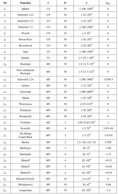
ABC-AMR is evaluated using a standard benchmark suite on numerical optimization problems consisting of 30 functions [1], [2], [18]. Table 1 presents a brief overview on each of the 30 standard benchmark functions. More details on each benchmark function can be found in [1]. The benchmark suite consists both unimodal (f1−f9) and multimodal (f10−f30),
separable (e.g., f1, f3, f15, f16) and non-separable (e.g., f2, f4, f14,
f17), high (f1−f18) and low (f19−f30) dimensional functions. To
optimize a multimodal function, the search algorithm must possess both exploitative and explorative characteristics so that it can explore the locally optimal points without being trapped around any of them. Some of the multimodal functions can have hundreds of local minima, even when the dimensionality is just two or three. The number of local optima usually increases exponentially with the number of dimensions, which makes their optimization extremely difficult. For example, the Ackley function f13 has one narrow
global minimum basin, but with exponentially many minor local minima. The Griewank function f14 has a component
Table 1: Standard benchmark functions. D: dimensionality, S: search space, fmin: function value at global
minimum, C: function characteristics — U: Unimodal, M: Multimodal, S: Separable, N: Non-separable.
No Function C D S fmin
f1 Sphere US 30 [-100, 100]D 0
f2 Schwefel 2.22 UN 30 [-10, 10]D 0
f3 Schwefel 2.21 US 30 [-10, 10]
D
0
f4 Schwefel 1.2 UN 30 [-100, 100]
D
0
f5 Powell UN 24 [-4, 5]
D
0
f6 Dixon-Price UN 30 [-10, 10]
D
0
f7 Rosenbrock UN 30 [-30, 30]
D
0
f8 Step US 30 [-100, 100]
D
0
f9 Quartic US 30 [-1.28, 1.28]
D
0
f10 Rastrigin MS 30 [-5.12, 5.12]
D
0
f11
Non-continuous
Rastrigin MS 30 [-5.12, 5.12]
D
0
f12 Schwefel 2.26 MS 30 [-500, 500]D -12569.5
f13 Ackley MN 30 [-32, 32]D 0
f14 Griewank MN 30 [-600, 600]D 0
f15 Alpine MS 30 [-10, 10]D 0
f16 Weierstrass MS 30 [-0.5, 0.5]D 0
f17 Penalized MN 30 [-50, 50]D 0
f18 Penalized2 MN 30 [-50, 50]D 0
f19 Foxholes MS 2 [-65.53,65.53]D 1
f20 Kowalik MN 4 [-5, 5]D 3.07e-04
f21
Six Hump
Camel Back MN 2 [-5, 5]
D
-1.0316
f22 Branin MS 2 [-5, 10] x [0, 15] 0.398
f23 Hartman3 MN 3 [0, 1]
D
-3.86
f24 Hartman6 MN 6 [0, 1]D -3.32
f25 Shekel5 MN 4 [0, 10]D -10.15
f26 Shekel7 MN 4 [0, 10]
D
-10.40
f27 Shekel10 MN 4 [0, 10]D -10.54
f28 Fletcher-Powell MN 10 [-π, π]D 0
f29 Michalewicz MS 10 [0, π]
D
-9.66
f30 Langerman MN 10 [0, 10]
D
Table 2: Performance of the proposed algorithm ABC-AMR, compared to the basic ABC algorithm on the benchmark functions. Results are averaged over 50 independent runs. Better performance by ABC-AMR is
marked with boldface font. In case the performance difference is not significant by t-Test
with at least 95% level of confidence (i.e., α = 0.95), it is marked as “Similar”.
No fmin
ABC ABC-AMR
Better Performance
(t-Test with α = 0.95) Mean Error Std. Dev. Mean Error Std. Dev.
f1 0 3.58e–11 8.14e–12 4.15e–11 3.89e–12 Similar
f2 0 1.04e–14 5.33e–14 1.87e–14 7.80e–15 Similar
f3 0 9.37e+00 3.22e+00 8.65e+00 1.95e+00 Similar
f4 0 2.75e–10 2.49e–10 3.09e–10 8.71e–11 Similar
f5 0 2.50e+00 9.25e–01 8.26e+00 8.33e–01 ABC
f6 0 6.67e–01 8.74e–02 5.01e–03 1.69e–03 ABC-AMR
f7 0 2.75e+00 8.08e–01 3.17e+00 6.24e-01 Similar
f8 0 0 0 0 0 Similar
f9 0 8.61e–13 7.07e–13 7.23e–13 2.02e–13 Similar
f10 0 5.79e–15 2.48e–15 6.58e–15 2.90e–15 Similar
f11 0 8.82e–09 2.33e–09 7.23e–09 2.51e–09 Similar
f12 -12569.5 3.49e+02 1.18e+02 1.06e+02 3.26e+01 ABC-AMR
f13 0 3.08e–06 3.96e–07 6.03e–08 9.58e–09 ABC-AMR
f14 0 4.35e–08 8.47e–09 3.99e–08 1.78e–08 Similar
f15 0 6.90e–06 2.15e–06 6.82e–06 1.93e–06 Similar
f16 0 3.03e–02 8.69e–03 7.36e–02 8.59e–03 ABC
f17 0 5.82e–08 9.42e–09 7.11e–12 2.43e–12 ABC-AMR
f18 0 2.64e–03 8.53e–04 2.49e–03 7.25e–04 Similar
f19 1 0.03 0.013 0.02 0.045 Similar
f20 3.07e–04 7.60e–05 6.69e–06 6.56e–05 7.80e–06 Similar
f21 –1.0316 0.00 0.00 0.00 0.00 Similar
f22 0.398 0.00 0.00 0.00 0.00 Similar
f23 –3.86 0.00 0.00 0.00 0.00 Similar
f24 –3.32 0.00 0.00 0.00 0.00 Similar
f25 –10.15 0.30 0.11 0.28 0.06 Similar
f26 –10.40 0.02 0.0025 0.03 0.021 Similar
f27 –10.54 0.12 0.045 0.04 0.0051 ABC-AMR
f28 0 8.05 2.89 7.95 1.46 Similar
f29 –9.66 0.00 0.00 0.00 0.00 Similar
local minima which are far from the single global minimum. The low dimensional functions f19−f30 have fewer local
minima, but they are well separated and distant, making them difficult to be explored without being trapped around them.
Table 2 presents the results of ABC-AMR with the basic ABC [1] algorithm. For the high dimensional functions f1–f18,
the common parameters are set as — population size SN=50, maximum number of function evaluations FE=100000 and limit=100. For low dimensional f19–f30, SN=100, FE=10000
and limit=10*D. Each algorithm made 50 independent runs on each function. The mean and standard deviation of the best found solutions from different runs are reported in Table 2. Following points summarize our observations on the results.
Out of the 30 functions f1–f30, ABC-AMR performs
better than ABC on five functions, while ABC performs better only on three functions. On the remaining 22 functions, their results are similar (i.e., the performance difference is not statistically significant in t-tests with at least 95% degree of confidence). Thus the overall performance of ABC-AMR is better than ABC.
The unimodal functions f1–f9 and low dimensional
functions f19–f30 are relatively easier to optimize. On
these functions, the performance of ABC and ABC-AMR are mostly similar.
On the high dimensional multimodal functions f10–f18,
which are the most complex function family for any algorithm, the performance of ABC-AMR is much better than ABC. On almost all these functions, ABC-AMR performs either better or equally well to the basic ABC algorithm. This indicates that more explorations, as performed by ABC-AMR, are necessary for good performance on these multimodal functions with exponentially many locally optimal points.
In summary, ABC-AMR is better suited than the basic ABC algorithm on more complex multimodal and high dimensional functions.
6.
CONCLUSION
This paper introduces ABC-AMR — a novel variant of the basic ABC algorithm and evaluates its performance on several standard benchmark functions. Results indicate that ABC-AMR can perform better than ABC on more complex functions which require more search space explorations. There might be several possible ways to further improve ABC-AMR. Firstly, ABC-AMR uses a simple strategy to control the mutation rate. Some more sophisticated scheme, possibly parameterized by the current maturity of the search process, may improve the algorithm further. Secondly, ABC-AMR tries more to improve the explorations only. Putting some emphasis on exploitations, especially around the best-so-far candidate solutions, may further improve the results. Thirdly, the quality of the final solution might be improved further by using an efficient local searcher after the execution of ABC-AMR is over. Finally, ABC-AMR has been applied only on the benchmark continuous optimization problems. It would be interesting to study how well ABC-AMR performs on many other existing problems, especially the discrete and real world ones. Some interesting examples of discrete and real world problems on which ABC-AMR could be employed are industrial process control [6], machine learning [10], bioinformatics [35], data
mining [36], telecommunications [37], engineering analysis and design [38] and many others [11].
7.
REFERENCES
[1] D. Karaboga and B. Basturk, On the performance of artificial bee colony (ABC) algorithm, Applied Soft Computing8 (1) (2008) 687–697.
[2] D. Karaboga, An idea based on honey bee swarm for numerical optimization, Erciyes University, Kayseri, Turkey, Technical Report-TR06, 2005.
[3] D. Karaboga and B. Akay, A comparative study of artificial bee colony algorithm, Applied Mathematics and Computation214 (1) (2009) 108–132.
[4] S. Sobti and P. Singla, Solving travelling salesman problem using bee colony based approach, International Journal of Engineering Research and Technology2 (6) (2013) 186–189.
[5] K. Naidu, H. Mokhlis and A.H.A. Bakar, Multiobjective optimization using weighted sum Artificial Bee Colony algorithm for Load Frequency Control, International Journal of Electrical Power and Energy Systems 55 (2) (2014) 657–667.
[6] R. Mukherjee, D. Goswami and S. Chakraborty, Parametric optimization of Nd:YAG laser beam machining process using artificial bee colony algorithm, Journal of Industrial Engineering, vol. 2013, Article ID 570250, 15 pages, 2013. DOI: 10.1155/2013/570250.
[7] H. Garg, Solving structural engineering design optimization problems using an artificial bee colony algorithm, Journal of Industrial and Management Optimization,10 (3) (2014) 777–794.
[8] Z. Zhao, D. Yin and Y. Jiang, Improved bee colony algorithm based on knowledge strategy for digital filter design, International Journal of Computer Applications,
47 (2) (2013) 241–248.
[9] A. Mishra, A. Khanna, N. Singh and V. Mishra, Speed control of DC motor using bee colony optimization, Universal Journal of Electrical and Electronic Engineering 1 (3) (2013) 68–75.
[10]A. Karegowda and M. Darshan, Optimizing feed forward neural network connection weights using artificial bee colony algorithm, International Journal of Advanced Research in Computer Science and Software Engineering
3 (7) (2013) 452–454.
[11]A. Bolaji, A. Khader, M. Betar and M. Awadallah, Bee colony algorithm, its variants and applications: A survey, Journal of Theoretical and Applied Technology 47 (2) (2013) 434–459.
[12]T. Park and K. R. Ryu, A Dual population genetic algorithm for adaptive diversity control, IEEE Trans. Evolutionary Computation 14 (6) (2010) 865–884. [13]R. K. Ursem, Diversity guided evolutionary algorithms,
in Proc. 7th Int. Conf. Parallel Problem Solving from Nature (PPSN), 2002, pp. 462–474.
[15]V. Tereshko, A. Loengarov, “Collective Decision-Making in Honey Bee Foraging Dynamics”, Comput. Inf. Sys. J., vol. 9, no. 3, pp. 1–7, 2005.
[16]M. Abd, A cooperative approach to the artificial bee colony algorithm, in Proc. IEEE Congress on Evolutionary Computation (CEC), 2010, pp. 1–5. [17]W. Lee and W. Cai, A novel artificial bee colony
algorithm with diversity strategy, in Proc. 7th Int. Conf. Natural Computation, 2011, pp. 1441–1444.
[18]B. Wu and S. Fan, Improved artificial bee colony algorithm with chaos, in Computer Science for Environmental Engineering and Eco-Informatics, Part I, Communications in Computer and Information Science, eds. Y. Yu, Z. Yu and J. Zhao, vol. 158, 2011, pp. 51–56.
[19]L. Fenglei, D. Haijun and F. Xing, The parameter improvement of bee colony algorithm in TSP problem, Science Paper Online, Nov. 2007.
[20]G. Zhu and S. Kwong, Gbest-guided artificial bee colony algorithm for numerical function optimization, Applied Mathematics and Computation 217 (7) (2010) 3166– 3173.
[21]F. Kang, J. Li, Z. Ma and H. Li, Artificial bee colony algorithm with local search for numerical optimization, Journal of Software 6 (3) (2011) 490–497.
[22]E. Montes and R. Koeppel, Elitist artificial bee colony for constrained real-parameter optimization, in Proc. IEEE Congress on Evolutionary Computation, 2010, pp. 1–8.
[23]H. Quan and X. Shi, On the analysis of performance of the improved artificial bee colony algorithm, in Proc.4th Int. Conf. Natural Computation (ICNC), 2008, 654–658. [24]F. Qingxian and D. Haijun, Bee colony algorithm for the
function optimization, Science Paper Online, Aug. 2008. [25]S. Kumar, V. Sharma and R. Kumari, A novel crossover
based artificial bee colony algorithm for optimization, International Journal of Computer Applications 82 (8) (2013) 18–25.
[26]Y. Xu, P. Fan and L. Yuan, A simple and efficient artificial bee colony algorithm, Mathematical Problems in Engineering, vol. 2013, Article ID 526315, 9 pages, 2013. DOI: 10.1155/2013/526315.
[27]N. Sulaiman, J. Saleh and A. Abro, A modified artificial bee colony (JA-ABC) optimization algorithm, in Proc. International Conference on Applied Mathematics and
Computational Methods in Engineering (AMCME), 2013, pp. 74–79.
[28]A. Abro and J. Saleh, Enhanced global-best artificial bee colony optimization algorithm, in Proc. 6th European Symposium on Computer Modeling and Simulation, 2012, pp. 95–100.
[29]W. Gao, S. Liu and L. Huang, A global best bee colony algorithm for global optimization, Journal of Computational and Applied Mathematics 236 (11) (2012) pp. 2741–2753.
[30]W. Gao and S. Liu, A modified artificial bee colony algorithm, Computers and Operations Research 39 (3) (2012) pp. 687–697.
[31]20 W. Gao and S. Liu, Improved artificial bee colony algorithm for global optimization, Information Processing Letters111 (17) (2011) pp. 871–882. [32]G. Zhu and S. Kwong, Gbest-guided artificial bee colony
algorithm for numerical function optimization, Applied Mathematics and Computation217 (7) (2010) pp. 3166– 3173.
[33]A. Abro and J. Saleh, An enhanced artificial bee colony optimization algorithm, Recent Advances in Systems Science and Mathematical Modelling, ed. D.S. Nikos Mastorakis, Valeriu Prepelita, 2012: WSEAS Press.
[34]A. Banharnsakun, T. Achalakul and B. Sirinaovakul, The best-so-far selection in artificial bee colony algorithm, Applied Soft Computing11 (2) (2011) pp. 2888–2901. [35]C. Lin and S. Su, Using an efficient bee colony algorithm
for protein structure prediction, Int. Journal of Innovative Computing, Information and Control 8 (3b) (2012) 2049–2064.
[36]M. Abdulsalam and A. Bakar, A cluster based deviation detection using the artificial bee colony (ABC) algorithm, International Journal of Soft Computing7 (2) (2012) 71–78.
[37]A. Ozen and C. Ozturk. "A novel modulation recognition technique based on artificial bee colony algorithm in the presence of multipath fading channels, in Proc. IEEE 36th International Conference on Telecommunications and Signal Processing (TSP), 2013, pp. 239–243. [38]B. Akay and D. Karaboga, Artificial bee colony