Comparative Study of different Methodologies to Predict
Human Character
Ankur M. Bobade
M.E Digital Electronics PRMIT&R, Badnera, India
N. N. Khalsa
Asst. Professor (EXTC Deptt) PRMIT&R, Badnera, India
ABSTRACT
Realistic data modeling can be used to predict human performance and explore the relationships between diverse sets of variables. A major challenge of realistic data modeling is how to simplify or anticipate the findings with a limited amount of pragmatic data to a broader perspective. In this paper, the individuality of some of the categorization methods that have been effectively applied to handwritten script recognition and results of SVM and ANNs categorization method, applied on handwritten script. After preprocessing the handwritten image the psychological individuality in the writing namely size, slant and pressure, baseline, number of breaks, margins, speed of writing and spacing between the words is extracted. These attributes are subsequently provided to Neural classifier and into support vector machine for categorization. In neural classifier, it is discovered that three ways of combining decisions of various MLP’s, designed for various attributes. To exhibit the method and the value of modeling human performance with SVM, SVM applied to a real world human factors problem of identification of character of a person. The results specify that the SVM based model of person’s character detection gives good performance. Various propositions on modeling human character by using SVM have been discussed. From machine learning an approach is introduced, known as support vector machine (SVM), which can help deal with this challenge.
General Terms
Character detection, script detection, attributes, etc.
Keywords
Human character predicting model, human character data analysis and modeling, support vector machine (SVM), categorization.
1.
INTRODUCTION
Human character predicting modeling has several benefits for the study of human machine interaction and system design. Such modeling can help predict human character and lead system design. Much attention has been dedicated to this area of research [3], and a wide range of models has been developed, from behavior level (such as Optimistic, positive attitude, ambitious, Practical, controlled, Closeness of sentiment and intelligence, emotionally unsettled, unpredictable, etc) to processes underlying human performance (such as detailed depiction of cognitive processes) [4] [6]. Human character predicting models include both theoretical modeling and empirical data modeling (often called realistic modeling). Usually, theoretical modeling starts with and tests definite theories regarding human performance, which are then revised and polished on the basis of realistic data. On the other hand, realistic modeling is usually more data driven from the beginning and proceeds by finding the
finest mathematical method to build up a quantitative function between human character and realistic data and variables. The human character recognition area has found attention to categorization scheme depends on learning from examples approach, particularly based on artificial neural networks (ANNs) since the early 1990s. Fresh learning schemes, using support vector machines (SVMs), are now dynamically studied and applied in human character recognition problems. Learning schemes have beneficiated character recognition methods tremendously. Comprehensive analysis of the broad field of human character predicting modeling can be seen in, e.g., [8]. In many states of affairs, yet resultant theories may not exist, and hence, realistic modeling is needed to predict human character and resolve the related specific practical issues. The approach may also recommend impending into the realm of analysis and may provide as a basis for future theory augmentation.
The modern gush in the advancement in human character recognition has grant publications but doesn’t involve the performance comparison of artificial neural networks and support vector machines regarding same attributes set for handwritten script. This paper produced the outcomes of ANN and SVM applied on handwritten script. The advantages and limitation of these categorization schemes will also be discussed.
2.
CHALLENGES AND
METHODOLOGIES
A major challenge of realistic modeling is how to generalize or extrapolate the findings with a limited amount of observed data to a broader context. This challenge arises because it is often impossible or impractical to collect data on all the possible situations of a human behavior. Researchers and practitioners often need to extrapolate or generalize their findings beyond the scope of their realistic study.
In human factors, the most extensively adopted method for investigating and modeling the relationships among realistic variables is the family of linear and polynomial least squares kernel methods. These methods are extensively used to evaluate realistic data and to predict human character as a function of assorted variables by establishing the finest fit of a model to the pragmatic data. However, these methods have restricted capability to approximate nonlinear relationships and thus cannot grant a good fit of the observed nonlinear data [5] [7].
support for extrapolation and generalization purposes in human attributes research.
Fascinatingly, the field of machine learning faces alike challenge in its investigation on the relationship between training data and other non-training data. In machine learning, in addition to conventional kernel methods, artificial neural network (ANN) is a widely used nonlinear modeling method for kernel analysis and categorization [10] [13]. This method is based on biological or genetic neural networks. The main specialty of ANN as a kernel analysis method is its ability to approximate a continuous function by minimizing the error in fitting a limited amount of pragmatic data [14]. In machine learning, this error is called training error, and the set of observed data is called training data.
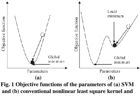
(a) (b) Fig. 1 Objective functions of the parameters of (a) SVM
and (b) conventional nonlinear least square kernel and ANN
The question is which method can be used to develop the best model to approximate the real model? While it is impossible for us to know the real model, these methods cannot be evaluated by comparing the developed models with the real model. A main criterion of evaluating these developed models is their generalization performance, which refers to a model’s accuracy in predicting output values based on input variables of present/future data rather than training data. The integrity to fit in modeling the training data does not guarantee the integrity to fit in present/future data due to the presence of noise, which is often called overfitting [15]. In machine learning, the error of models in predicting future data is called generalization error or testing error.
Recently, in machine learning, a new kernel method known as support vector machine (SVM) has been urbanized and applied to help develop generalization performance [16]. SVM is a group of supervised learning methods that can be applied to categorization or kernel, and uses statistical learning theory as a general mathematical framework with a limited amount of data [17] [18]. Unlike conventional kernel methods and ANN, SVM develops models by minimizing the upper bound of the generalization error rather than minimizing the training error [19].
This gives SVM a greater ability to generalize. Improving generalization performance and minimizing the error in fitting training data are both optimization processes, whose success depends on the individuality of the employed optimization functions. The objective function of the parameters of SVM based models is a quadratic function as shown in Fig. 1(a), which only has one global minimum. Thus, most optimization parameters of SVM based models can be explore accurately. In other words, SVM does not suffer from the problem of
“being trapped” at local minima. Compared to SVM, the objective functions of the parameters of conventional nonlinear kernel and ANN are likely to have a nature as shown in Fig. 1(b) and can possibly trap the search process into a local minimum. In other words, the explore process can possibly never find the global minimum. Table I reviews some individuality of the methods discussed earlier.
Generalization performance is an important aspect in estimating the different kernel methods. The basic idea to estimate the generalization performance of one method is that testing data and training data should be different. In practice, K-fold cross validation is widely used [20] [21]. Generally, R2 (coefficient of determination) and root mean square (rms) error (rmse) are selected as performance pointers. The larger is the R2value, the larger is the proportion of the variation in
the dependent variables that is explained by the models. Similarly, the lesser is the value of rmse, the lesser is the prediction error of the models, representing enhanced performance.
Table I. Comparison of Realistic Modeling Methods
Constraints SVM ANN Polynomial
kernel
Linear kernel
Linear relation modeling ability
Strong Strong Moderate No
Optimization criterion
Upper bound of
generalization error
Training error
Training error
Training error
Robust to local minima
Yes No No No
Level of expertise required
Expert Expert Moderate Easy
Here following, initially introduce the basic principle of SVM, as well as the SVM based modeling approach. After that, to show how to apply SVM based modeling in human attributes research, SVM used to model the probability of script detection with human character predicting systems. Consequently, the generalization performance of the SVM based model with a model based on Stevens’ law, along with some models developed with ANN, polynomial kernel, and linear kernel is evaluated. Finally, the significance of the SVM based modeling approach as an option for human character modeling discussed and propose some suggestions on how to use SVM to predict human character.
3.
SUPPORT VECTOR MACHINE
BASED MODELING
3.1
Fundamental Principle of SVM
Assume the following training data set {xi, yi}, i = 1, . . . , l ; xi∈ R
d
; yi∈ R d
(1) Where xi be a vector of input variables and yi signifies the
actual obtained output values for all the training data and that is as flat as possible.
Here in the case of linear functions, f(x) can be
f(x) = ω • x + b (2)
Where • signifies the dot product, ω is the weight vector, and b is constant. Smoothness in the case of (2) can be accomplish by minimizing the Euclidean mean of the weight vector ω, i.e. ω. formally, this problem can be expressed as a convex optimization problem
Minimize 2
Subject to yi f (xi) ≤ ε
f(xi) yi ≤ ε. (3)
Sometimes, though, such a function that fits all the observed data with ε precision does not exist.
Likewise, the slack variables ξi and ξi∗ are established to
address the infeasible constraints of the optimization problem (3). SVM not only minimizes the training error by minimizing the sum of ξi and ξi∗ but also minimizes ω in order to increase
the smoothness of the function. This optimization problem can be expressed as [17]
Minimize 2 + C ∗ Subject to yi f (xi) ≤ ε + ξi
f(xi) yi≤ ε + ξi
ξ∗i, ξi ≥ 0; C > 0 (4)
Where C is constant, determining the tradeoff between the smoothness of the function and the training error. This is related with handling a ε-insensitive loss function
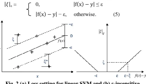
ε = 0, ≤ ε
− ε, otherwise. (5)
Fig. 2 (a) Loss setting for linear SVM and (b) ε-insensitive loss function
Fig. 2(a) shows the loss setting diagrammatically, and Fig. 2(b) shows the ε-insensitive loss function. A major reason for using the ε-insensitive loss function is that it can produce a sparse set of SVs, which makes realistic computation achievable. Despite, other loss functions such as Huber, Gaussian, and Laplace loss functions do not produce a sparse set of SVs, making the computation complex, if not infeasible. A in depth analysis and discussion of these different loss functions can be found in [22].
The convex optimization problem (4) can be solved more easily in its twin form in most cases. After (4) is transformed into a twin objective function, it takes the following form [44]:
Minimize 0.5 αi − α∗i) (αj − α∗j) (xi • xj)
+ i (αi − α∗i) − ε αi − α∗i)
Subject to αi − α∗i) =0 0≤ αi; α *
i≤C (6)
Where αi and α∗i are Lagrange multipliers for the ith training example and are gained by solving (6). Only some of the coefficients (αi− α∗i) are nonzero, and the corresponding input
vectors xi are called SVs. These SVs xi and the corresponding
nonzero Lagrange multipliers αi and α∗i give the values of
weight vector ω, which can be expressed as
ω = αi− α∗i) xi (7)
By combining (2) with (7)
f(x) = αi − α∗i) (x • xi) + b (8)
Moreover, the bias parameter b can be computed by applying Karush Kuhn Tucker conditions [18]. Equation (8) is the linear model developed with this method.
Though, in most realistic cases, the relationship between input variables and output values is not linear. The SVM based nonlinear model can be developed by simply mapping input variables into a high dimensional feature space F (i.e., by a map Φ : Rd→ F) [17]. The nonlinear function is formed as
follows:
f(x) = ω • ϕ(x) + b. (9)
With the same process of solving the linear function f(x) = αi− α∗i) (ϕ (x) • ϕ (xi)) + b. (10)
However, as the input dimensions increase, the dimensions in the feature space further increase by many crease, and thus, the mapping process become a computationally infeasible problem. This problem can be deal with by defining appropriate kernel functions in place of the dot product of the input vectors in the high dimensional feature space [36]. The kernel function is expressed as
K(x, xi) = ϕ (x) • ϕ (xi). (11)
Combining (10) with (11), the kernel function that takes the following general form:
f(x) = αi− α∗i) K(x, xi) + b. (12)
At present, numerous type of kernel functions have been defined and used, such as linear functions, polynomial functions, and radial basis functions (RBFs). Among these, the RBF, as defined in the following, is most usually used:
K(x, xi) = exp
(13)
Where 1/2σ2 represents the width of the RBF.
3.2
Execution Method
After the model is built, it can be used to predict the target value based on input variables of new data. This can be implemented with the command “svmpredict” in the LIBSVM package [24].
3.3
Example
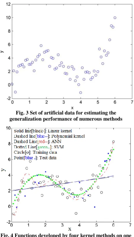
To demonstrate that the integrity of fit in the training data does not mean the integrity of fit in other data and that SVM tends to illustrate a superior ability to generalize, this method estimated functions from a set of artificial data shown in Fig. 3, by using linear kernel, polynomial kernel, ANN, and SVM, respectively. A threefold cross validation employed to evaluate the generalized performance of these different methods.
Initially, the collected data set was erratically divided into three subsets. Then, three models for each of the four modeling methods were built. Each model used two subsets of the data as a training set by leaving out one subset each time. Finally, the average of the errors associated with the left out subsets was used as an estimate of the generalization error, whereas the mean of the errors associated with the training sets was used as an estimate of the training error.
Fig. 3 Set of artificial data for estimating the generalization performance of numerous methods
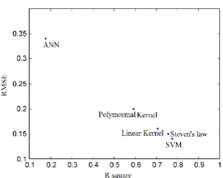
Fig. 4 Functions developed by four kernel methods on one training data set
RBF was used as the kernel function of SVM. By estimating the SVM based model for a wide range of the width of the
RBF kernel (1/2σ2
), cost coefficient (C), and loss function parameter (ε), the final parameters were determined: 1/2σ2=
0.1, C = 100, and ε = 1. The three models based on SVM were then each obtained with one of the three training sets according to these final parameters by using “svmtrain” in the LIBSVM package. The hide function of ANN was taken as RBF for the comparison with SVM based models.
The three training data sets were used to build three groups of models. Each group contains four models, built with the four kernel methods. Fig. 4 shows one group of the models. Fig. 5 shows the generalization performance (+) and the training performance (◦) corresponding to each method with the two performance indicators rmse and R2(higher values of R2and lower values of rmse represent better performance).
Fig. 5 (+) Generalization performance and (◦) training performance of each method
As illustrated in Fig. 5, ANN has the best training performance. It does not, however, have the best generalization performance. This is because ANN has a strong ability to approximate continuous functions by minimizing the training error, and thus, ANN overfits the training data. Although SVM does not show the best training performance, it has the best generalization performance. This is because SVM can make a tradeoff between the training error and its ability to approximate continuous functions so as to minimize the upper bound of the generalization error rather than minimizing the training error, and thereby avoid overfitting. Linear and polynomial kernels show worse training performance than SVM and ANN because they do not have enough ability to fit the training data. In addition, linear and polynomial kernels do not have good generalization performance in this case. One reason for this is that, according to [15], the generalization error of the functions is equal to or less than the sum of the training error and a nonnegative term, and linear and polynomial kernels show worse training performance in this case. Another possible reason is that the objective function of the parameters of polynomial kernel did find the local minimum rather than the global minimum.
4.
SVM VS NEURAL NETWORKS
Place SVM and Neural classifiers illustrate various assets in the following respects.
among the samples. SVMs be trained via quadratic programming (QP), and the training period is usually proportional to the square of number of samples. Several quick SVM training techniques with almost linear complication are available.
Flexibility of training: The assets of neural classifiers can be attuned in layout level training by gradient descent by the desire of optimizing the universal performance [23]. Here, the neural classifier is embedded in the layout recognizer for character recognition. Conversely, SVMs can barely be trained at the level of holistic patterns.
Model selection: The simplification or generalization performance of neural classifiers is sensitive to the size of structure, and the selection of a proper structure relies on cross validation. The convergence of neural network training undergoes from local minima of error outside. Conversely, the QP learning of SVMs assuredly finding the universal most favorable. The SVMs performance depends on the selection of kernel type and kernel assets, but this dependence is less influential.
Categorization accuracy: SVMs established greater categorization accuracies to neural classifiers in several researches.
Storage and execution intricacy: SVM learning by QP intermittently outcome in a large number of SVs, which ought to be stored and computed in categorization. Neural classifiers contain a lot less parameters, and the number of parameters is easy to control. In brief, neural classifiers occupy lesser storage and computation than SVMs.
5.
MODELING THE PROBABILITY OF
SCRIPT DETECTION WITH HUMAN
CHARACTER PREDICTING SYSTEMS
In this section, SVM method is applied to a real world human factors challenge in the context of human character predicting system from handwriting. The primary objective of the systems is to extract data from various attributes such as size, slant and pressure, baseline, number of breaks, margins, speed of writing and spacing between the words, and subsequently provided to Neural classifier and into support vector machine and others for categorization. In human character predicting system design and evaluation, the main objective of developing models is to help researchers estimate script detection performance without spending a significant amount of time designing experimental materials, recruiting subjects, and conducting experiments. Because the physical characteristics of images generated by human character predicting systems can be measured by image based metrics, which greatly impact detection performance, script detection performance can be modeled as a function of image metrics with these human character predicting systems.
Several studies have investigated modeling the relation between script detection and the metrics of images generated by human character predicting systems. In the following, probability of script detection models as a function of image metrics using SVM and compare the modeling results with those of the model based on Stevens’ law and the models developed by linear kernel, polynomial kernel, and ANN, respectively.
Fig. 8. Generalization performance of the five methods
6.
MODELING THE PROBABILITY OF
PREDICTING HUMAN CHARACTER
AND RESULTS
After the values of the image metrics and detection probabilities were collected, the rms, RPOT, and Doyle metrics took as input variables to model the probability of script detection and predicting human character by using SVM and other methods.
First fourfold cross validation used to estimate the generalization performance of these different methods. The collected data were randomly divided into four partitions. The kernel function of SVM was selected as the RBF kernel. By evaluating the SVM based model for the wide range of parameters [including the width of the RBF kernel (1/2σ2
), the cost coefficient (C), and the loss function parameter (ε)], the final parameters were determined: 1/2σ2= 1, C = 10, and ε =
0.15. According to the values of these parameters, the final SVM based model can be built with the collected data by using the command “svmtrain” in LIBSVM. Furthermore, fourfold cross validation method applied to estimate the performance of the models developed by Stevens’ law, linear kernel, polynomial kernel, and RBF ANN.
The results of the two performance indicators of all the models as a function of the rms, RPOT, and Doyle metrics are shown in Fig. 8. The performance of the SVM based model is almost identical to, even slightly better than, that of the model developed on the theoretical basis of Stevens’ law. The linear kernel model shows relatively good performance in this case, very possibly because the relationship between detection probability and the three metrics is close to linear, in contrast to the strongly nonlinear relationship between variables shown in the illustrative data set in Fig. 4.
7.
CONCLUSION
This is because SVM can make a tradeoff between minimizing the training error and its ability to approximate continuous functions so as to minimize the upper bound of the generalization error. This gives SVM a greater ability to generalize. In practice, SVM based modeling may be perceived for some modelers as too difficult to use. However, several software tools exist such as the LIBSVM package that can be used quite easily for this purpose. Thus, it suggest that, for better generalization performance in human attributes modeling and data analysis, SVM based modeling should be considered an important option. A feasible method is to try linear kernel and polynomial kernel first; if their generalization performance is not satisfactory, SVM based modeling can then be utilized.
8.
REFERENCES
[1] C. Wu, Y. Liu, and C. Walsh, “Queueing network modeling of a realtime psychophysiological index of mental workload—P300 in evoked brain potential (ERP),” IEEE Trans. Syst., Man, Cybern. A, Syst., Humans, vol. 38, no. 5, pp. 1068–1084, Sep. 2008. [2] Y. Liu, R. Feyen, and O. Tsimhoni, “Queueing
network-model human processor (QN-MHP): A computational architecture for multitask performance,” ACM Trans. Hum. Comput. Interact, vol. 13, no. 1, pp. 37–70, Mar. 2006.
[3] L. Allender, “Modeling human performance: Impacting system design, performance, and cost,” in Proc. Mil., Gov. Aerosp. Simul. Symp., Adv. Simul. Technol. Conf., Washington, DC, 2000, pp. 139–144.
[4] Y. Liu, “Queuing network modeling of elementary mental processes,” Psychol. Rev., vol. 103, no. 1, pp. 116–136, Jan. 1996.
[5] Champa H. N. and K. R. Ananda Kumar. 2010. Automated Human Behavior Prediction through Handwriting Analysis. First International Conference on Integrated Intelligent Computing.
[6] Ball G.R., Stittmeyer R. and Srihari S. N. 2010. Writer verification in historical documents. Proceedings Document Recognition and Retrieval XVII San Jose, CA, SPIE.
[7] Champa H N and K R Ananda Kumar. Handwriting Analysis for Writer’s Personality Prediction. Intl. Conference on Biometric Technologies and Applications- the Indian perspective. Biometrics India Expo New Delhi India. pp. 182-191.
[8] K. A. Gluck and R. Pew, Modeling Human Behavior With Integrated Cognitive Architectures: Comparison, Evaluation, and Validation. Mahwah, NJ: Lawrence Erlbaum, 2005.
[9] M. Bauerly and Y. L. Liu, “Computational modeling and experimental investigation of effects of compositional elements on interface and design aesthetics,” Int. J. Hum.-Comput. Stud., vol. 64, no. 8, pp. 670–682, Aug. 2006.
[10]Z. Liu, R. E. Torres, N. Patel, and Q. Wang, “Further development of input-to-state stabilizing control for
dynamic neural network systems,” IEEE Trans. Syst., Man, Cybern. A, Syst., Humans, vol. 38, no. 6, pp. 1410– 1433, Nov. 2008.
[11]E. Asua, V. Etxebarria, and A. Garcia-Arribas, “Neural network-based micropositioning control of smart shape memory alloy actuators,” Eng. Appl. Artif. Intell., vol. 21, no. 5, pp. 796–804, Aug. 2008.
[12]A. Cevik, M. A. Kutuk, A. Erklig, and I. H. Guzelbey, “Neural network modeling of arc spot welding,” J. Mater. Process. Technol., vol. 202, no. 1–3, pp. 137–144, Jun. 2008.
[13]S. J. Wu, N. Gebraeel, M. A. Lawley, and Y. Yih, “A neural network integrated decision support system for condition-based optimal predictive maintenance policy,” IEEE Trans. Syst., Man, Cybern. A, Syst., Humans, vol. 37, no. 2, pp. 226–236, Mar. 2007.
[14]S. Haykin, Neural Networks: A Comprehensive Foundation, 2nd. Englewood Cliffs, NJ: Prentice-Hall, 1998.
[15]O. Bousquet, S. Boucheron, and G. Lugosi, “Introduction to statistical learning theory,” in Advanced Lectures on Machine Learning. New York: Springer-Verlag, 2004, pp. 169–207.
[16]M. Cimen, “Estimation of daily suspended sediments using support vector machines,” Hydrol. Sci. J., vol. 53, no. 3, Jun. 2008.
[17]V. Vapnik, The Nature of Statistical Learning Theory. New York: Springer Verlag, 1995.
[18]V. Vapnik, Statistical Learning Theory. New York: Wiley, 1998.
[19]C. J. C. Burges, “A tutorial on support vector machines for pattern recognition,” Data Mining Knowl. Discovery, vol. 2, no. 2, Jun. 1998.
[20]O. Bunke and B. Droge, “Bootstrap and cross-validation estimates of the prediction error for linear regression models,” Ann. Statist., vol. 12, no. 4, pp. 1400–1424, Dec. 1984.
[21]D. J. Spitzner, “Constructive cross-validation in linear prediction,” Commun. Statist.—Theory Methods, vol. 36, no. 5, pp. 939–953, Apr. 2007.
[22]A. J. Smola and B. Scholkopf, “A tutorial on support vector regression,” Statist. Comput, vol. 14, no. 3, Aug. 2004.
[23]C. L. Liu, K. Marukawa, Handwritten numeral string recognition: character level training vs. string level training, Proc.7th ICPR, Cambridge, UK, 2004,Vol.1. [24]C. C. Chang and C. J. Lin, LIBSVM, A Library for
Support-Vector-Machines.Available: http://www.csie.ntu.edu.tw/~cjlin/libsvm/