Performance Evaluation of Fractionally spaced constant modulus algorithm (FS-CMA) in Relation to CMA (Constant modulus algorithm) method for blind equalization of wireless signals

(1)

Performance Evaluation of Fractionally

spaced constant modulus algorithm

(FS-CMA) in Relation to CMA (Constant

modulus algorithm) method for blind

equalization of wireless signals

Dr. JKR Sastry

[email protected]

KL University, Vaddeswaram, Guntur District Mr. T Rambabu

[email protected] Andhra University, Visakhapatnam

Dr. P Rajesh Kumar [email protected] Andhra University, Visakhapatnam

-ABSTRACT

---Wireless communication is being used for many purposes and has become very frequently used mode of communication. Blind equalization methods are being used to estimate the received signal without the necessity to use the trained sequences in the input. Many methods CMA (Constant Modulus Algorithm), FS-CMA (Fractionally spaced CMA), PC-CMA(Phase compensation CMA), MMA(Multi-Modulus Algorithms) are being used for blind equalization. However all the methods are affected due to Inter symbol interference (ISI) and Bit error rate(BER) in the transmission.It has been proved [9] that CMA performs reasonably well compared to LMS methods in the absence of trained sequences. However the method suffers from issues such as Partial spacing, non-phase compensation etc.

In this paper the performance evaluation of FS-CMA in comparison to CMA considering the model parameters at which the maximum performance can be achieved is presented. The performance of FS-CMA as against CMA in respect toInter Symbol interference ISI[1] and Bit error rate (BER), considering optimum parameters has also been presentedin this paper.

Key words:FS-CMA, CMA, ISI, BER, Blind equalization, wireless communication, Model parameter, optimum model parameters

--- Date of Submission: 28th_Jul₂₀₁₃_Date_of_Acceptance:_August_23,₂₀₁₃

---

I. Introduction

W

ireless communication is being used for many purposes and has become very frequently used mode of communication. But the wireless communication gets affected due to various types of noises that include multipath effect, inter symbol interference, inter carrier interference, co-channel interference, ambiguity in transmission of bits etc. The noises limits channel bandwidth and time varying multipath propagation [4]. The method of receiving data without prior knowledge of transmitting information is called as blind equalization.

Many types of filters and algorithms are in use to affect blind equalization. CMA (Constant modulus algorithm)

[2, 3] is most frequently used algorithm for affecting blind equalization which has many limitations such as lack of phase compensation, fractional spaced diagonal compensation etc.

Fractional-Spaced Constant Modulus Algorithm (FS-CMA) [5] is an improved algorithm over CMA algorithm [2,3]. CMA does not compensate for phase losses.

The Fractional Spaced Equalizer (FSE) [6, 7] is the parallel combination of a number of Baud Spaced Equalizers (BSE).

(2)

If T is the symbol period, then tap spacing =T/M, where M is the sampling factor.

The source symbols are taken from a finite M array real alphabet of zero mean which means that all symbols are equally probable. In this method second order statistics are taken as signal model.

Fig. 1.1 represents the mathematical model for fractional spaced (T/2) equalizer [8].

Figure 1.1:Diagram of the T/2 spaced Equalizer model

Where, !_"impliesbaud spacedsource symbolat

sampleindex n and Cisthevector

r e p r e s e n t i n g thefractionallyspaced channel impulse response.#_$istheadditivewhiteGaussianchannel noise, f is thevector that containstheFS-equalizer coeﬃcients. The output of the equalizer which is Y_&is fractional spacedequalizeroutput. The number ofcoefficientsinthechannel vector Cis '₍ and equalizer

responsevector fisN₎. Thesystemoutputis given by

*_"=sT(n)+₎+wT(m) f(1.1) (1.1)

The length of the input sequence is given by

S (n) = [,_"_,,_"-.… ,_"– ', 1 134_(1.2)

The vector of baud spaced source symbols is given by

'₅6 78'₉1 '_:; 1</23 (1.3)

The vector of additive zero mean white Gaussian noise with variance σω is expressed by

#8=< 6 7#_$#_$-.… #_$; '_:1 134_(1.4)

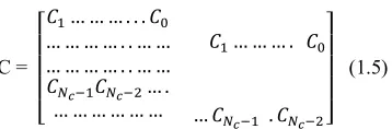
The Cis the Ns*N₎decimated channel convolution matrix expressed as

C =

> ? ? ?

@+.… … …. . .+A

… … … …. .… …

+_B_C_-.+_B_C_-D….

… … … …

+_.… … …. +_A

… +_B_C_-. .+_B_C-DEF

F F G

(1.5)

In this model, Fractional spaced equalizer is included.The cost function for such a model is given by

H_(IJ_K_.6 1/LMNO||P_Q|R_{; P}_|S_T(1.6)

Where U is a fixed constant, the parameters p, q are the positive integers. In this method p=2 and q=2 are taken for the second order statistics for implementation of the T/2 – spaced equalizer. The weights are updated by minimizing the cost function. Therefore the steepest gradient descent algorithm is obtained by the following expressions.

F (n+1) =f(n)-ug(w(n)) (1.7) g (w(n)) = VW_8X<Y_8P

"< (1.8) Y8P_") = - Z_[_\1/4 (|P_"|D_{; P<}D_{6 P}

"8P ;|P"|D< (1.9) Where ‘f’ is the length of equalizer, r (n) is the receiver input vector and µ is the step size, Y8P_"< is the error function. Where U is taken as

P 6 NO|!_"|]_T_/_NO_|_!

"|DT (1.10)

For improvement of the computational efficiency, an additional step is used to update the equation of the channel equalizer. The signed error (SE) function is simplified by eliminating multiplication operation. The equation is modified as

f (n+1) = f(n)-^ r(n) sgn(_8PX<<(1.11)

The cost function is given by

H_(IJ_`_,_`6 NOa|PX|; baT (1.12)

And corresponding updated equation is given by

c8X 1 1< 6 c8X< ; ^V8X<,dX8P_"8b-|P_"|<< (1.13)

Assumingβ = √U, the eq. (3.12) becomes

H_ef-(IJ6 NO|aP"|; √*aT (1.14)

Selection of Uis important, as it has great bearing on convergence. The dissipation constant U is given the value of U 6 h_iD_{, where h}

i is the jkl positive member of the source alphabet and integer ν is represented as

j 6 hVd=mX_no8n-./D8.pq

rs s-.st

(3)

satisfies the fractional spaced equalizer. The cost function of the FS-CMA equalizer is given by eq. (3.16).

H_ue-(IJ6 NO||!4_{+c 1 #}4_c_|_{; √*}_|_T(1.16)

Therefore the eq. (3.16) is the cost function which justifies the error values of the desired output which is processed by the adaptive filters at the decision block.The channel model of 4-QAM [70] source is used in fractional spaced equalizer which is shown in the fig. 1.2.

Figure 1.2: Block diagram of Channelmodelfora

4-QAM source.

The channel outputofa 4-Q A M source is given by eq. (1.17).

v8X< 6 ∑x h_"

"yA z8{ ; X| ; {A< 1 #8{< (1.17) The Fig.1.2 represents distributed complexdata

{a_&Tsentbythe transmitterovera linear time

invariantc h a n n e l withimpulseresponseh(t). The

receiverattemptsto recoverthe inputdatasequence{a_&Tforchanneloutputx (t)inwhich T

i s thesymbol period. w (t) is channel noise existence in thechanneloutput, whichiszeromeanstationary. Thecomplex and white Gaussianwith variance

‘σD_{~isindependentofthechannelinputh}

". The model

considers thecomplexdataandnoise and bothsatisfiessymmetricproperty, that is E {h_"D_{T= E {•}

kD} =0 and EO|h_"|]_{T -2N}D_O_|_h

"|DT<0, i.e. thekurtosis K(h") ofh_{"i s negativeasisoftenthecaseofQAM system.}

Dueto thepresenceofISI, t he recoveryofinputsignal requiresthatthechannelimpulse response h (t−T_A<be identifiedin Decision Feedback Equalizer(DFE).

In

fractionalblindequalizationsystem,thechanneloutputsamp ledat theknownbaudrate1/T, the transmitted symbol sequence and received samples at the c h a n n e l output of 6-tap coefficients are shown in the eq. (1.18).

v8X|< 6 € h_nz8X| ; •| ; {_A< 1 #8X|<

x

ny-x

6 h_"W z8X| ; {_A< 1 #8X|< (1.18)

The eq. (3.18) can be written as discrete convolution with noise form as given by the eq. (1.19).

‚8X< 6 ∑x h_nz_"-n1 #_"

ny-x (1.19) Based on this relationship, traditional linear FSE are designed as FIR filter θ (ƒ-._{< =∑} _„

n B

nyA ƒ-nto be applied on ‚_"to remove the ISI from the equalizer output P_"=∑B „_n

nyA ‚"-n. The equalizer algorithm attempts to adjust the parameterO„nTnyAB .

The FS-CMA aims to minimize the cost function given in eq. (1.20).

H_D8„<= .

]NO8|P"|D; …D<DT (1.20) Where

…_D6f†8|Q‡|ˆ‰

fO8|Q‡|sT (1.21) The above expression of the cost function represents the error values substituted into a 4-QAM channel after adding the noise, which forms second order statistics.

II. Performance Analysis of FS-CMA

The FS-CMA equalization has been analyzed considering different model parameters which include SNR, Sample size, step size. Several experiments have been conducted using the FS-CMA algorithm to determine the MSE (Mean Square error) and observe the convergence of the same for effecting the symbol realizations and draw the constellations.

Experiments have been conducted varying the maximum sample size from 500 to 4000 and varying the SNR from 10dB to 30dB. For carrying the analysis, 4-QAM is used for affecting the modulation.

In this section performance analysis of FS-CMA is carried to determine the effectiveness of equalization at a particular SNR and sample size. The best performance parameters (SNR and sample size) are then selected and the same are used to determine the performance of CMA.

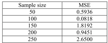
Table 2.1 shows the mean square error at the output with varying steps of 50 samples out of maximum sample size of 500 when SNR kept at 10dB.

Table 2.1 Variance of MSE when maximum sample size is 500 and SNR fixed at 10dB.

Sample size MSE

50 0.5936

100 0.0818

150 1.8192

200 0.9451

250 2.6500

€ a_&

x

"y-x

δ8t

;nT<

‚8{<

6 €

a

&

x

h

8 t

h(t)

chan

(4)

300 0.4358 350 2.0721 400 2.1544 450 0.0852 500 0.8478

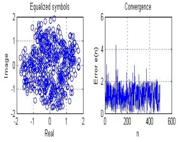
Fig.2.1 and 2.2 show the Graphs related to symbol equalization and MSE convergence when the sample size is 500 and SNR = 10Db

Figure 2.1 Symbol equalization Figure 2.2 MSE Convergencewhen Maximum sample size is 500 and

SNR = 10 Db

Table 2.2 shows the mean square error at the output with varying steps of 50 samples out of maximum sample size of 500 when SNR is kept at 15dB

Table 2.2 Variance of MSE when maximum sample size is 500 and SNR fixed at 15dB

Sample size MSE

50 0.0028 100 0.0987 150 0.0518 200 0.2219 250 0.0499 300 2.2548 350 0.3535 400 0.0582 450 0.2303 500 2.5568

Figures at 2.3 and 2.4 show the Graphs related to symbol equalization and MSE convergence when the sample size is 500 and SNR = 15Db

Figure 2.3 Symbol equalization Figure 2.4 MSE Convergencewhen Maximum sample size is 500 and SNR = 15Db

Experiment has been carried further by changing SNR for different sample sizes.

Table 2.3 shows the mean square error at the output with varying steps of 50 samples out of maximum sample size of 1000 when SNR is kept at 10 dB

Sample size MSE

100 3.1897 200 3.2562 300 0.2523 400 1.2796

500 1.4643

600 0.4112 700 2.6040

800 0.4112

900 1.9656 1000 0.6768

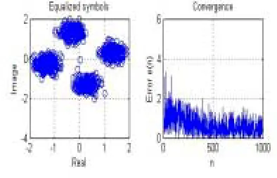
Fig.2.5 and 2.6 show the Graphs related to symbol equalization and MSE convergence when the sample size is 1000 and SNR = 10Db

(5)

Table 2.4 shows the mean square error at the output with varying steps of 50 samples out of maximum sample size of 1000 when SNR is kept at 15dB

Sample size MSE

100 2.3860 200 1.4366 300 0.1164 400 0.0000 500 0.5700 600 2.3901 700 0.0399 800 0.6441 900 0.3925 1000 0.1357 Fig.2.7 and 2.8 show the Graphs related to symbol

equalization and MSE convergence when the sample size is 1000 and SNR = 15Db

Figure 2.7 Symbol equalization Figure 2.8 MSE Convergencewhen Maximum sample size is 1000 and SNR = 15Db

III. Estimation of optimum model parameters in respect of FS-CMA and analysis of performance of CMA at the optimum parameters

Series of such experiments have been carried by varying the sample sizes from 500 to 3600 and SNR 10dB to 25 dB. The mean square errors achieved for each pair of model parameters considering SNR and Sample size have been shown in the Table 3.1

Table 3.1 Mean square errors for different sample sizes and SNR in respect of FS-CMA

SN

R(

d

B

)

MS

E

(500

sa

mple

s)

MS

E

(1000

sa

mple

s)

MS

E

(2000

sa

mple

s)

MS

E

(3000

sa

mple

s)

MS

E

(3600

sa

mple

s)

10 0.8478 0.6768 0.0137 0.3486 0.0177

15 2.5568 0.1357 0.8175 0.1126 0.1163 20 3.0328 0.0857 0.3725 0.0053 0.0729 25 0.0490 0.0205 0.0001 0.0164 0.0165

Table 3.2 Mean square error computed at SNR = 25dB,

Population sample Size = 2000 and Blind equalization method = CMA

Sample size MSE

200 1.5800

400 0.3150

600 1.8395

800 2.3765

1000 0.5617

1200 1.3780

1400 0.1083

1600 6.1876

1800 0.7087 2000 0.1919

From the Table 3.1, it can be seen that FS-CMA has perfectly converged when SNR is 25dB and sample size is 2000. The error at this point is quite negligible (0.0001). The performance of CMA has been analyzed at this point.

Table 3.2 shows the MSE convergence and Figures 3.1 &3.2 shows the symbol realization and MSE convergence with Sample size fixed at 2000 and the dB at 25 and the blind equalization method being CMA. It can be seen from the Fig 3.1 and Fig. 3.2 that behavior of CMA is erratic at SNR=25Db and the sample size = 2000 as the convergence of MSE is varying and not smooth. Even the symbols are not realized properly in this case which can be seen from the figure 3.1. Thus, it can be concluded that FS-CMA performs much better than CMA for realizing the symbols at the output of the channel considering most efficient converging point (SNR= 25dB and Sample size = 2000).

Figure 3.1 Symbol equalization Figure 3.2 MSE Convergence

(6)

IV. Comparative Performance Analysis of FS-CMA and CMA considering ISI and BER

The comparison of performance by FS-CMA and CMA has been further carried by considering BER and ISI. The convergence of BER with reference to different SNR at sample size fixed at 2000 and the convergence of ISI keeping the SNR at 20db have been studied to find how effective the FS-CMA is with reference of CMA blind equalization algorithm.

Table 4.1 shows the computation of BER, at different SNR ranging from 10dB to 25dB keeping the sample size at 2000 considering both FS-CMA and CMA.

Figure 4.1 represents the BER behavior using CMA

and FS-CM Algorithms for the blind channel equalization keeping the sample size fixed at 2000. It can be seen from the figure that the BER has declined quite considerably when compared to CMA as the signal to noise ratio has been increasing.

From the Table 4.1 it can also be concluded that BER converges much faster in case of FS-CMA when compared to CMA at the converging point being 2000 samples.

Table 4.1: Performance Comparison of BER Vs SNR for CMA and FS-CMA at 2000 samples. S.No SNR FC-CMA(BER) CMA(BER)

1 10 10-0.02₁₀-0.06

2 12 10-0.04₁₀-0.08

3 14 10-0.6 10-1

4 16 10-0.8₁₀-1.2

5 18 10-2₁₀-2.4

6 20 10-3.4₁₀-3.8

7 22 10-5₁₀-5.4

8 24 10-7.2₁₀-7.6

Figure 4.1: Plot of the BER Vs SNR using CMA and FS-CMA.

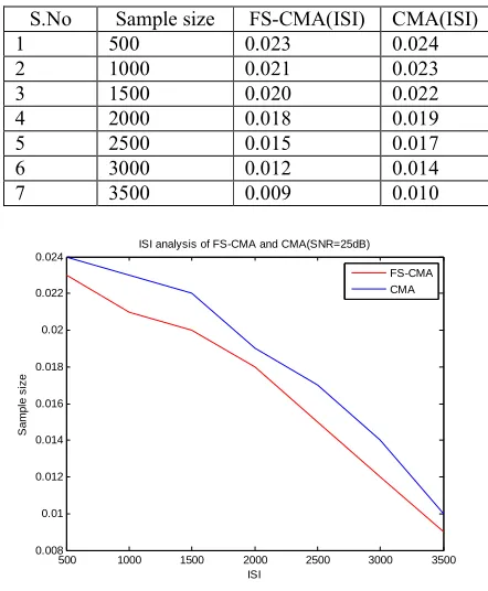
Further comparison of performance of CMA and FS-CMA has been carried with reference to ISI keeping SNR at 20dB and varying the sample sizes. Table 4.2 shows the behavior of ISI when sample size is varied keeping the SNR fixed at 20dB. It can be seen from the Table 4.2 that ISI converges much faster in case of FS-CMA when compared to FS-CMA keeping the SNR fixed at 20dB.

Table 4.2: Performance Comparison of ISI for CMA

and FS-CMA at SNR=20dB

S.No Sample size FS-CMA(ISI) CMA(ISI)

1 500 0.023 0.024

2 1000 0.021 0.023

3 1500 0.020 0.022

4 2000 0.018 0.019

5 2500 0.015 0.017

6 3000 0.012 0.014

7 3500 0.009 0.010

Figure 4.2: Plot of the ISI Performance comparison of

the CMA and FS-CMA.

Fig.4.2 represents the ISI performance using CMA and

FS-CMA Algorithm for the blind channel equalization, keeping the SNR at 25dB. It can be seen from the graph that the inter symbol interference converges and reduces must faster as the number of signal samples increases in case of FS-CMA.

V. Conclusions

It is evident from the plots that fractionally spaced equalizer shows better response than CMA considering the MSE, BER and ISI. The FS-CMA gives better results when SNR is fixed at 20dB and the sample size at 2000. BER converges to lower side as the SNR increases and similarly ISI converges to lower side as the sample size increases. Thus FS-CMA proved to perform much better considering all the three dimensions (MSE, BER, and ISI).

10 12 14 16 18 20 22 24

0 0.1 0.2 0.3 0.4 0.5 0.6 0.7 0.8 0.9 1

SNR

BE

R

BER analysis of FC-CMA and CMA(sample size=2000)

FC-CMA CMA

500 1000 1500 2000 2500 3000 3500 0.008

0.01 0.012 0.014 0.016 0.018 0.02 0.022 0.024

ISI

Sa

m

p

le

s

ize

(7)

References

[1]. G.D. Forney Jr., “Maximum likely-hood sequence of digital sequences in the presence of inter-symbol interference, IEEE transactions on information theory, Vol. 18, 1971, pp: 363-378.

[2]. Oraizi, H. and S. Hosseinzadeh, “A novel marching algorithm for radio wave propagation modeling over rough surfaces,” Progress In Electromagnetics Research, PIER vol.57, pp 85– 100, 2006.

[3]. N. K Jablon, “Joint Blind Equalization, Carrier Recovery, and Timing Recovery for High-Order QAM Signal Constellations” IEEE Trans. Signal Processing, vol. 40, no. 6, pp. 1383—1398, 1992. [4]. L. Garth, J. Yang, and J. J. Werner, “Blind

equalization algorithms for dual-mode CAP–QAM reception,” IEEE Trans. Communication., vol. 49, pp: 455–466, Mar. 2001.

[5]. Thakallapalli, S. R., S. R. Nelatury, and S. S. Rao, A new error function for fast phase recovery of QAM signals in CMA blind equalizers," IEEE Workshop on Statistical Signal Processing, pp: 70-73, 2003.

[6]. K. N. Oh and Y. O. Chin, “Modified constant modulus algorithm: Blind equalization and carrier phase recovery algorithm,” in Proc. ICC ’95, Seattle, WA, June 18–22, 1995, pp: 498–502. [7]. Jones, A.E. and Gardiner, J.G., Phase error

correcting vector modulator for personal communications network (PCN) transceivers, Electronics Letters, vol.27, no.14, pp.1230-1231, July 1991