Vehicle Active Suspension System performance using
Different Control Strategies
Atef, Mahmoud M
#1, Soliman, M-Emad S.
*2, Sharkawy, A.B.
#3Department of Mechanical Engineering, Assuit University, Egypt.
Abstract: The objective of the present work is to investigate the performance of an active suspension system of a typical passenger car through the application of three different control strategies under three different road irregularities. Tested control strategies are PID, LQR and FLC. Road irregularities considered are: a single rectangular pothole, a single cosine bump, and an ISO class-A random road disturbance. A 2-DOF quarter-vehicle model is used to simulate, evaluate and compare performance of these controllers against each other and against the original passive suspension system. Both tire gripping force and actuator force were normalized with respect to vehicle weight to recognize tire separation and enhance readability and interpretation of results. Simulation results showed that, active suspension systems are advantageous compared to passive ones. Active suspension implementing FLC control surpassed both PID and LQR controllers. Improvement of ride comfort was recognized by a reduction of sprung mass displacement and acceleration up to 23.8% and 52% respectively compared to the passive case. Improvement of load capacity is clear with a suspension travel reduction up to 61%. Moreover, vehicle stability was enhanced by increasing the tire separation margin up to 28 % of vehicle weight. An actuator force up to 39.5% of vehicle weight is required. All achieved by active suspension implementing FLC control.
Keywords: - Vehicle active suspension system, FLC, PID, LQR.
I. INTRODUCTION
The main task of a vehicle suspension is to provide passenger ride comfort, safe road handling together with an acceptable load capacity. Ride comfort is achieved by isolating the chassis mass from road disturbances while road handling is achieved by preventing the wheels from loosing road contact [1]. Load capacity depends on suspension system deflection (suspension travel). A luxury vehicle suspension will provide a high comfort level but would significantly reduce the stability of the vehicle at turns, lane change manoeuvres, or during negotiating an exit ramp. On the other hand, a high performance suspension system will yield good vehicle handling, at the expense of ride comfort [2].
Generally, vehicle suspensions are classified into three categories: passive, active and semi-active [3]. In passive systems, the vehicle chassis is supported
by only springs and dampers with fixed parameters. Passive means the system just dissipates kinetic energy with no external energy input. In Semi-active suspensions, no energy is supplied into suspension system but the damper is a controllable, variable damping one which is automatically adjusted based on control strategy. For active suspension, the damper and spring are interceded by a force actuator which adds energy to the system in order to suppress sprung mass oscillation of vehicle. The force actuator can be controlled by various types of controllers to achieve the desired performance [4], [5].
A good design of an optimal passive suspension can work up to some extent with respect to optimized riding comfort and road holding ability, but cannot eliminate this compromise [6]. Several studies have shown that this conflict can be eased by using active suspension systems instead of passive ones. Demands for better ride comfort and good road handling has motivated many automotive industries to consider the use of active suspension systems. However, although active suspension systems are superior in performance to passive suspensions, their physical realization and implementation is generally complex and expensive, requiring sophisticated electronically operated sensors, actuators and controllers [2]. The actuator in an active suspension system is controlled by various types of controllers determined by the designer. The correct control strategy should reduce the displacement and acceleration of the sprung mass and provide adequate suspension deflection to maintain tires on contact with road and maximize load capacity. Thus, the improvement of active vehicle suspension systems via controller design has attracted more interest and become a promising subject of research and development in the last decade.
and longitudinal dynamics (pitch motion of vehicle) [4], [11].
A number of active vehicle suspension control strategies has been studied and/or proposed by researchers. Agharkakli et al [3] investigated the application of an LQR controller to an active suspension system. The model used was a quarter vehicle model. A single cosine and repeated cosine bumpy profiles were input as road disturbances. They concluded that active suspension systems implementing linear quadratic regulator (LQR) gave lower amplitudes and faster settling time for sprung-mass displacement and acceleration, suspension travel, and wheel deflection compared to passive ones. However, performance was evaluated for a discrete, limited single cosine bump but not for a standard real road (ISO random road profile) which is more representative and realistic [3]. Kumar [6] tested the performance of an active suspension system using a proportional integral derivative (PID) controller whose gains are tuned using Zeigler and Nichols tuning rules. A quarter vehicle model has been used. A unit step and an ISO random road were used as road disturbances. He reported that the PID-based active suspension system improved ride comfort but with no appreciable improvement in road holding [6]. Changizi et al [12] compared the performance of active suspension system using PID and FLC controllers based on a quarter vehicle model. A unit step input was used as road disturbance. Their active suspension system using the fuzzy logic control (FLC) controller performed better than when using the PID controller. However, road handling performance was not evaluated in their work [12] . Sharkawy [13] compared the performance of an active suspension system under LQR, FLC and adaptive FLC controllers. A quarter vehicle model has been used to investigate the suspension behaviour under a unit step input and a varying frequency sine wave as road disturbances. He concluded that the performance quality in a descending order was adaptive FLC, FLC and LQR respectively[13]. Other control strategies such as PID Controller tuned by Back Propagation Neural Network [8], adaptive neuro active force control [14] and Fuzzy logic controller optimized by genetic algorithm [15] have been proposed for active suspension systems.
In this paper, a quarter-vehicle model has been used to simulate, evaluate and compare performance of an active suspension system of a passenger vehicle under three different proposed controllers. These controllers are PID, LQR and FLC. Road disturbances were modelled as three different disturbance types: rectangular pothole, single cosine bump and an ISO (class A) random road disturbance. Comparison was made of system behaviour under these controllers against each other and against the original passive suspension system.
II. SUSPENSION SYSTEM MODEL:
A 2-DOF quarter vehicle model has been used. This model consists of a sprung mass representing one quarter of total vehicle body mass and an unsprung mass which refers to the mass of one wheel assembly. Suspension system between sprung and unsprung masses is modelled as a combination of a linear viscous damper and a linear spring element. Tire has been modelled by its equivalent stiffness while tire damping is neglected. In the proposed active suspension system, an actuator is inserted between the sprung mass and the unsprung mass, which is able to generate a control force that plays important role in comfort and controlled motion of vehicle. The Quarter vehicle model is shown in Figure (1).
Fig.1: Quarter vehicle model a) passive suspension system b) active suspension system
Applying Newton’s second law of motion, the dynamic equations of motion could be derived as [13]:
(1)
(2)
Let’s define the following state variables as:
Equations (1) and (2) can be arranged in state space form as:
(3)
Where
,
,
Where Ms is the sprung mass, Mus the unsprung
mass, Cs the damping coefficient, ks the spring
stiffness, kt the tyre stiffness, ua the actuator force, zs
displacement (both measured from static equilibrium position) , zr the road profile, zs–zus the suspension
deflection (suspension travel) ,zus–zr the tire
deflection , the sprung mass velocity and is
the unsprung mass velocity. Model parameters are given in table(1) [6].
Table1 Quarter vehicle model parameters.
Parameter Value
Sprung mass, Ms 290 kg
Unsprung mass, Mus 60 kg
Spring stiffness, ks 16.8 kN/m
Tyre stiffness, kt 190 kN/m
Damping coefficient, Cs 1 kN.s/m
III.DESIGN DETAILS OF PROPOSED CONTROLLERS
1)PID controller:
Block diagram of the proposed active suspension system using PID controller is shown in figure (2).
Fig. 1: Block diagram of the proposed PID controller for active suspension system.
The control input U (t) is given by:
(4)
Where kp is the proportional gain, kd is the derivative
gain, ki is the integral gain and e (t) is the resulting
error. The PID controller was tuned using Zeigler-Nichols rules [17].
2)LQR controller:
LQR is a technique in modern control theory that uses state-space approach to analyse systems. State-space simplifies analysis of a multi-output system. In state variable form, mathematical model of an active suspension system can be expressed as:
(5)
For optimal design of a state variable feedback (SVFB ), we may define the controller’s performance index, J as [3]:
(6) where Q and R in LQR denote weighting factors or penalties for smooth trajectory(xTx) and minimal power consumption (uTu).
An SVFB regulator for a system is expressed as
(7)
where K is the state feedback gain matrix.
For optimal design the SVFB matrix K should be selected such that the performance index J is minimized [18] .
Linear optimal control provides the solution of Equation (6). The gain matrix K is computed from [1]:
(8)
Where the matrix P is determined by the solution of Algebraic Riccati Equation (ARE) [2]:
(9)
For proposed LQR controller, the parameters in matrices Q and R were found by trial and error to be:
, R=0.01
Using the Matlab function (lqr) for solving ARE, the value of the SVFB matrix k is:
3) FLC controller
A fuzzy control system is a system which emulates a human expert. Creating machines to emulate human expertise in control gives a new way to design controllers for complex plants whose mathematical models are hard to specify. The knowledge of the human operator would be put in the form of a set of fuzzy linguistic rules[19]. The fuzzy logic controller consists of three steps: fuzzification, fuzzy inference and defuzzification. Fuzzification is a Process of defining the fuzzy sets, and determination of the degree of membership of crisp inputs in appropriate fuzzy sets. Fuzzy inference is a process of evaluation of fuzzy rules to produce an output for each rule and aggregation or
combination of the outputs of all rules.
Defuzzification is a process of conversion of aggregate output fuzzy set to real-number (crisp) output values [15].
The FLC used in this work has two inputs and a single output. The two inputs are the suspension
travel (ZS-Zus) and the suspension velocity
. The output is the required actuator force
ua. This type of FLC is called fuzzy PD controller.
For the fuzzy inference step, product inference technique has been used, while centre-average method is used for defuzzification. The overall structure of the proposed FLC controller is shown in Figure(3) .Inputs and outputs are all normalized in the interval of [−1, 1] by scaling variables with
coefficients of Ss, Ssv for inputs and Su for output
Fig2: Block diagram of the proposed FLC suspension controller.
Each input and output has five Membership Functions (MFs). MFs of inputs and output are negative big (NB), negative small (NS), zero (Z), positive small (PS) and positive big (PB). The input MFs are equally spaced in the universe of discourse, and all MFs are described by a Gaussian function with width σ=0.2.The output has five singletons MFs having values of [-1 -0.5 0 0.5 1]. The rule base is represented by 25 rules with fuzzy terms derived from the designer’s knowledge and experience knowledge related to the system. They are listed in table (2) [13]. The rules of the fuzzy controller can read as follows:
Table2: FLC rule base
Force ua
Suspension travel (zs - zus)
NL NS Z PS PL
Suspension Velocity
NL NL NL NL NS Z
NS NL NL NS Z PS
Z NL NS Z PS PL
PL NS Z PS PL PL
PS Z PS PL PL PL
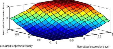
Using these MFs and rule base, the output surface of the fuzzy system is obtained as shown in figure (4).
-1 -0.5
0 0.5
1
-1 -0.5 0 0.5 1 -1 0 1
Normalized suspension travel Normalized suspension velocity
N
o
rm
a
li
ze
d
a
ct
u
a
to
r
fo
rce
Fig.4: Output surface of the fuzzy system
IV.RESULTS AND DISCUSSION:
In the present work, a quarter vehicle model of a vehicle suspension system has been used to simulate, evaluate and compare performance of three proposed
controllers, namely PID, LQR and FLC.
Performance has been compared for different road disturbances against a passive suspension system. The road disturbances used are a single rectangular pothole, a single cosine bump and an ISO random (class-A) road profile. Simulation has been
conducted for a vehicle speed of 16.67 m/s (60km/hr).
1) Rectangular pothole road disturbance:
Response of vehicle suspension system using proposed control to a sudden impact can be investigated with simple rectangular pothole. The pothole obstacle is mathematically modelled by the function [20]:
(10) where A is the pothole amplitude, L is the pothole length and s is the vehicle travelled distance (s=v*t). In this work, the pothole has amplitude A of 0.05 m and length L of 4 m. Rectangular pothole road input is shown in figure(5).
Fig. 5: Rectangular pothole road disturbance
1.1) Ride comfort results:-
Fig. 6: sprung-mass displacement- pothole disturbance.
Fig. 7: Normalized sprung-mass acceleration - pothole disturbance.
Table3: System recovery performance under different controllers. (Pothole disturbance)
Controller FLC PID LQR Passive
Settling time, ms
557 847 771 2648
Figure (6) depicts the sprung-mass displacement response for different controllers. It can be concluded from this figure that active suspension resulted in a significant reduction in peak value of sprung-mass displacement compared to the passive suspension case, which is desirable for better ride comfort. The best reduction of 23.8% was achieved with FLC controller, followed by 14.9% for LQR and 5.9% for PID. The FLC surpassed all other controllers regarding recovery performance or settling time as shown in table (3).
For sprung-mass acceleration, figure (7) shows that active suspension also significantly surpasses the passive case regarding peak acceleration values. Still FLC has a best reduction achievement of 61.3%, followed by 50% and 10.6% for PID and LQR respectively. Moreover, except for the LQR controller, sprung mass jerk or fluctuation of acceleration has been appreciably reduced when applying active suspension as shown in figure (8).
1.2)Road handling results:-
Fig.9: Normalized dynamic tire load- pothole disturbance.
Table 4: Best and worst tire gripping force values for different controllers (pothole disturbance)
controller passive LQR PID FLC
Best gripping force,% of vehicle weight
207.5 145 173 176
Worst gripping force, % of vehicle weight
7.4 51 31 24
Figure (9) represents the time response plot of dynamic tire force normalized with respect to vehicle weight. This force reflects the tire-road gripping force. A higher gripping force means better road handling and safety. Normalization with respect to vehicle weight aims to sensing the magnitude of this force and recognizing the case when tire separation or jump occurs. This results in better readability and interpretation of results. Figure (9) shows that tire separation margin has been improved with introduction of active suspension. Peak values
of total tire gripping force are shown in table (4). This table shows that LQR produced the highest tire-gripping margin of 51% of vehicle weight, followed by PID (31%) and FLC (24.1%). However, best road gripping force of (176% of vehicle weight) was produced by FLC followed by PID (173 %) and LQR (145%). Moreover, FLC has shown the fastest and best recovery behaviour after leaving hole.
1.3)Load capacity results:-
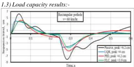
Fig. 10: suspension travel- pothole disturbance.
Figure (10) shows suspension travel variation with time. It is clear that, active suspension introduced an appreciable improvement in rattle space utilization. Note that a reduced suspension travel means higher load capacity of vehicle. FLC produced the largest
reduction of (37.1%) compared to passive
suspension, followed by LQR (35.4%) and PID (32.3%).
1.4) Actuator force results:-
Fig. 11: Normalized actuator force- pothole disturbance.
The actuator control forces generated by proposed controllers are compared in figure (11). Peak values of normalized actuator control force generated by FLC, PID and LQR are 77%, 98% and 111% of vehicle weight respectively. Therefore, FLC requires the smallest actuator force when implemented. Smaller force results in lower power consumption, a more compact design and a more realizable system.
2) A single cosine bump disturbance:
The single cosine bump input simulates a vehicle coming out of a smooth obstacle. A single cosine
bump is mathematically given by [20]:
a length of 4 m. Bumpy road input is shown in figure (12) [3].
Fig.12: A typical (single cosine bump) road disturbance input.
2.1)Ride comfort results:-
Fig.13: sprung-mass displacement- cosine bump disturbance.
Fig.14: Normalized sprung-mass acceleration- cosine bump disturbance.
Fig.15: sprung-mass jerk- cosine bump disturbance.
Table 5: System recovery performance under different controllers. (Cosine bump disturbance)
Controller FLC PID LQR Passive
Settling time, ms
466 777 746 2950
Figure (13) depicts the sprung-mass displacement response for different controllers. It can be observed from this figure that sprung-mass displacement peak
values in transient portion were 8.8, 9.7 and 10.1 cm for LQR, FLC and PID respectively. This is due to instant fast response of controllers. However, it can be concluded from this figure that active suspension resulted in a significant reduction in settling time, meaning fast recovery performance. The FLC surpassed all other controllers regarding settling time as shown in table (5).
For sprung-mass acceleration, figure (14) shows that active suspension significantly reduces the peak acceleration value. FLC has a best reduction achievement of 40.2%, followed by 35.6% and 32.2% for PID and LQR respectively. Moreover, sprung mass jerk has been appreciably reduced as shown in figure (15).
2.2)Road handling results:-
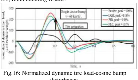
Fig.16: Normalized dynamic tire load-cosine bump disturbance.
Table 6: Best and worst tire gripping force values for different controllers (cosine bump road disturbance)
controller passive LQR PID FLC
Best gripping force, % of vehicle weight
209 218 256 261
Worst gripping force, % of vehicle weight
35.5 98
(Tire separati on)
159 (Tire separati on)
130 (Tire separati on)
2.3)Load capacity results:-
Fig.17: suspension travel- cosine bump disturbance.
Figure (17) shows suspension travel variation with time. It is clear that, active suspension introduced an appreciable improvement in rattle space utilization. Note that a reduced suspension travel means higher load capacity of vehicle. FLC produce the largest reduction of (36.7%) compared to passive suspension, followed by PID (32.2%) and LQR (25.3%).
2.4)Actuator force results :-
Fig.18: Normalized actuator force- cosine bump disturbance.
The actuator control forces generated by proposed controllers are compared in figure (18). Peak values of normalized actuator control force generated by FLC, LQR and PID are 122%, 132% and 165% of vehicle weight respectively. Therefore, FLC requires the smallest actuator force when implemented.
3) Random road profile disturbance:
A random exciting function has been found appropriate to model a real road surface as the main characteristic of a random function is uncertainty. The basic properties of random data in road model are described by Power spectral density (PSD). Random road profiles can be approximated by a PSD function in the form of [21]:
(12) Where Ω denotes the wave number in rad/m and
describes the value of PSD at reference
wave number =1 rad/m in m2/ (rad/m). The drop
in magnitude is modelled by waviness . By setting
waviness to =2, each class is simply defined by its
reference value . The ISO has proposed road
roughness classification (classes A-E) based on the power spectral density values [2].
A random profile of a single track can be
approximated by a superposition of sine
waves.
(11) where each sine wave is determined by its
amplitude and its wave number . By different
sets of uniformly distributed phase angles in
the range between 0 and 2π .and, s is the momentary position of vehicle. Amplitude of sine wave calculates form:
(14)
Where is wave number interval [20].
In this study, a road profile of class (A) was used as input to system. According to equations (13&14) road profile was generated by (N = 10) sine waves in the frequency range from 0.628 rad/m to 6.283
rad/m. The amplitudes were calculated and the
MATLAB function “rand” was used to produce uniformly distributed random phase angles in the range between 0 and 2π. Random road input is shown in figures (19&20).
Fig.19: Random road profile (ISO, class A)
Fig.20: Random road profile (ISO, class A), v=60 km/hr.
3.1)
Ride comfort results:-
Fig.22: Normalized sprung mass acceleration- ISO road profile.
Fig.23: Sprung mass jerk- ISO road profile.
The sprung-mass displacement for different controllers is shown in figure (21). It can be concluded from this figure that active suspension resulted in an improvement in ride comfort due to a significant reduction in peak values of sprung-mass displacement compared to the passive suspension case. The best reduction of 22% was achieved with the FLC controller, followed by 5% for PID and 1%for LQR.
For sprung-mass acceleration, figure(22) shows that active suspension also significantly suppresses the peak and root mean square (R.M.S) acceleration values. Still FLC has a best reduction in peak value achievement of 76.6%, followed by 76% and 60.2% for PID and LQR respectively. Also, FLC reduced R.M.S value by 61%, followed by 59.3% and 52% for PID and LQR. Moreover, sprung mass jerk has been appreciably reduced as shown in figure (23).
3.2)
Road handling results:-
Fig.24: Dynamic tire force- ISO road profile.
Table 7: Best and worst tire gripping force values for different controllers (ISO road profiles)
controller Passive LQR PID FLC
Best gripping
force, % of
vehicle weight
215 147 188.1 188.2
Worst gripping
force, % of
vehicle weight 47 (Tire separ -ation)
55 26 28
Figure (24) represents the time response plot of dynamic tire force normalized with respect to vehicle weight. Figure (24) shows that the tire separation margin has been improved with introduction of active suspension. Peak values of Total tire gripping force are shown in table (7). This Table shows that PID produced the highest margin of 26% of vehicle weight, followed by FLC (28%) and LQR (55%). However, best road gripping force of (188.2% of vehicle weight) was produced by FLC followed by PID (188.1 %) and LQR (147%).
3.3)
Load capacity results:-
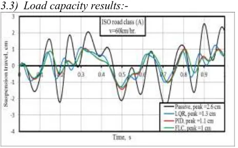
Fig.25: Suspension travel- ISO road profile.
Figure (25) shows suspension travel as a function of time. Active suspension introduced an improvement in rattle space utilization. FLC produce the largest reduction of (61%) compared to passive suspension, followed by PID (58%) and FLC (50%). Moreover, FLC has a best reduction in R.M.S value achievement of 52%, followed by 50% and 47.6% for PID and LQR.
3.4)
Actuator force results:-
Fig.26: Actuator force- ISO road profile.
V. CONCLUSIONS
Three control strategies (PID, LQR and FLC) have been tested for an active vehicle suspension system to improve the ride comfort, load capacity and road handling. A 2-DOF quarter vehicle model is used to simulate suspension performance. Three different road disturbances, namely, pothole, cosine bump and ISO class A random road profile were
used to evaluate and compare suspension
performance implying different control strategies. Simulation results showed that, active suspension resulted in a significant improvement of ride comfort, rattle space utilization and road safety. System performance when implementing FLC proved to surpass PID and LQR performance. FLC achieved maximum reduction in peak values of sprung mass acceleration for all road profiles followed by PID and then LQR, which means that FLC produced the best ride comfort performance. Moreover, The FLC surpassed all other controllers regarding recovery performance or settling time followed by PID and then LQR. However, LQR gave the highest tire gripping force (separation margin) followed by FLC and then PID for all road profiles. FLC has the best reduction in suspension travel for all road profiles followed by PID and then LQR. Therefore, FLC provided optimal utilization of rattle space. Another advantage of FLC is that it requires the smallest actuator force when implemented followed by PID and LQR. Therefore, FLC implementation means lower power consumption, a more compact design and a more realizable system.
REFERENCES
[1] F. L. Fisher, "Design of a Semi-active Controllable Electromagnetic Shock Absorber", Master of Science thesis, Northern Illinois University, Dekable, Illinois.2011
[2] S. Mouleeswaran, "Design and Development of PID Controller-Based Active Suspension System for Automobiles" PID Controller Design Approaches - Theory, Tuning and Application to Frontier Areas, M. Vagia, InTech, ,2012
[3] A. Agharkakli, G. S. Sabet and A. Barouz, ,"Simulation and Analysis of Passive and Active Suspension System Using Quarter Car Model for Different Road Profile", International Journal of Engineering Trends and Technology, 3 (5), pp.636-644. 2012 [4]R. B. Darus,, "Modeling and Control of Active Suspension for a Full Car Model", M. of Science thesis, University Technology Malaysia. 2008
[5]Q. Zhou, "Research and Simulation on New Active Suspension Control System", M. Science thesis, Lehigh University. , 2013. [6] M. S. Kumar and S. Vijayarangan,"Design of LQR Controller for Active Suspension System", Indian Journal of Engineering & Materials Sciences, 13 (June), pp.173- 179, 2006.
[7] A. A. Aldair and W. J. Wang,"Design and Intelligent Controller for Full Vehicle Nonlinear Active Suspension Systems", International Journal on Smart and Intelligent Systems 4(2), pp.224-243, 2011.
[8] M. Heidari and H. Homaei, "Design a PID Controller for Suspension System by Back Propagation Neural Network", Journal of Engineering, 2013 (241543 ), 2013.
[9] J. Z. Feng, J. Li and F. Yu,"GA-Based PID and Fuzzy Logic Control for Active Vehicle Suspension System", International Journal of Automotive Technology, 4 (4), pp.181-191, 2003. [11] M. Paksoy, R. Guclu and S. Cetin, "Semiactive Self-Tuning Fuzzy Logic Control of Full Vehicle Model with MR Damper", Advances in Mechanical Engineering, 2014.
[12] N. Changizi and M. Rouhani, "Comparing PID and Fuzzy Logic Control a Quarter-Car Suspension System", The Journal of Mathematics and Computer Science 3(3), pp.559-564, 2011. [13] A. B. Sharkawy,"Fuzzy and Adaptive Fuzzy Control for the Autombiles Active Suspension System", Vehicle system Dynamics, 43 (11), pp.795-806, 2005.
[14] G. Priyandoko, M. Mailah and H. Jamaluddin,"Vehicle Active Suspension System Using Skyhook Adaptive Neuro Active Force Control", Mechanical Systems and Signal Processing, 23 pp.855- 868, 2009.
[15] R. K. Pekokogoz, M. A. Gurel, M. Bilgehan and M. Kisa,"Active Suspension of Cars Using Fuzzy Logic Controller Optimized by Genetic Alograithm", International Journal of Engineering and Applied Sciences, 2 (4), pp.27-37, 2002. [16] Hung T. Nguyen, Nadipuram R. Prasad, Carol L. Walker, Elbert A. Walker, A First Course in Fuzzy and neural control, CRC Press, London, pp. 53-71, 2003.
[17] K. Ogata, Modern Control Engineering, Aeeizh, London, pp.681-745, ISBN: 0-13-043245-8: 0-13-043245-8, 2002. [18] M. Jamil, A. A. Janjua, I. Rafique, S. I. Butt, Y. Ayaz and S. O. Gilani,"Optimal Control based Intelligent Controller for Active Suspension System", Life Science Journal 2013;10(12s), 10 (12), pp.653-659, 2013.
[19]C.-y. Tang, G.-y. Zhao and Y.-m. Zhang, "The Application of Fuzzy Control Algorithm of Vehicle with Active Suspensions ", Research Journal of Applied Sciences, Engineering and Technology, 4 (16), pp.2744-2747, 2012.