http://www.sciencepublishinggroup.com/j/ccr doi: 10.11648/j.ccr.20170101.12
An Approximate Method to Find Changes in the Blood Flow
Rate Due to Planar Pathological Tortuosity of a Larger
Coronary Artery
Andriy Borysyuk
Department of Hydrodynamical Acoustics, Institute of Hydromechanics, Kyiv, Ukraine
Email address:
To cite this article:
Andriy Borysyuk. An Approximate Method to Find Changes in the Blood Flow Rate Due to Planar Pathological Tortuosity of a Larger Coronary Artery. Cardiology and Cardiovascular Research. Vol. 1, No. 1, 2017, pp. 7-17. doi: 10.11648/j.ccr.20170101.12
Received: January 30, 2017; Accepted: February 22, 2017; Published: March 15, 2017
Abstract:
Proceed from the analysis of coronarographies of patients with cardiac ischemia and cardiac syndrome X, anapproximate method is developed to allow cardiologists to find (with satisfactory precision and speed) both changes in the blood flow rate in larger coronary arteries, caused by the appearance of their planar pathological tortuosity, and a hemodynamic significance of those changes based on the data taken from the appropriate coronarographies only. This method is based on replacement of real blood flows in the originally healthy and subsequently pathologically tortuous artery with the corresponding cross-sectionally averaged ones, and subsequent calculation of the blood flow characteristics of interest in terms of the corresponding averaged flow characteristics. It allows one not to take account of a number of identical factors for the originally healthy and subsequently pathologically tortuous segment of the coronary artery under investigation, and gives one the possibility to determine the blood flow parameters of concern at any time after carrying out a coronarography. In addition, the developed method is not associated with solving complicated technical problems, and does not require special facility to be used, special professional training and significant expences. It was successfully tested in laboratory conditions and then successfully applied to appropriate patients.
Keywords:
Coronary Artery, Cardiac Syndrome X, Arterial Tortuosity, Blood Flow Rate1. Introduction
Coronary arteries (CA) are the vessels supplying myocardium with an oxygen-rich blood. They are the only sources of blood supply to the myocardium, and are situated both on the heart surface and within the myocardium constituting the so-called coronary tree. In this tree, there are the two main branches. These are the left branch (usually called the left coronary artery (LCA)) and the right one (ordinary referred to as the right coronary artery (RCA)).
The most severe and the most widely spread disease of coronary arteries is atherosclerosis [1, 2]. It is accompanied by depositing cholesterins and some fractions of lipoproteins on the inner surface of the vessel wall, with their subsequent calcification. As a result, in such coronary arteries fast local narrowings (i.e., stenoses) are formed, which, apart from the others, result in the blood flow
reduction in the arteries and possible further development of myocardial ischemia (MI).
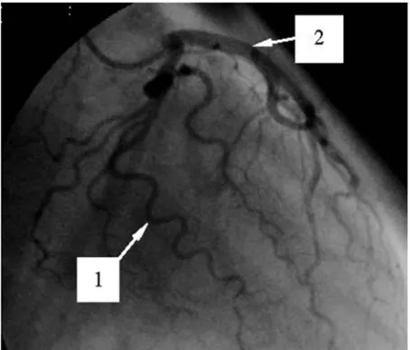
Figure 1. Coronarogram of the LCA with a severe pathological tortuosity of a few larger arteries.
According to the opinion of the dominant majority of researchers (see, for example, [5-14]), this tortuosity is the main reason for the appearance of the noted syndrome1. It is explained by the fact that the appearance of a pathological tortuosity in the originally normal (usually straight) segment of a coronary artery results in (i) an increase in the segment resistance to the blood motion; (ii) an additional pressure drop in the segment; (iii) an increase of the distance passed by blood in the segment2 and the corresponding increase of the viscous forces’ influence on the flow there, and hence, an increase in the blood flow energy dissipation, etc. All of these factors inevitably cause (apart from the other effects) a decrease in the blood flow velocity and rate in the coronary artery, and, under the appropriate circumstances, subsequent possible development of cardiac ischemia.
The discovery of the cardiac syndrome X and the ascertainment of the main reason for its initiation have stimulated reserachers to make the corresponding investigations. In those investigations, various aspects of fluid motion in channels with local tortuosity were studied.
1 The other resaons for the initiation of the cardiac syndrome X can be endothelial disfunction and/or microcirculatory disorders [1, 2, 5, 6, 9, 10, 14]. The first of them is associated with changes in the properties of endothelium (i.e., the inner layer of the vessel wall), and results in the corresponding changes in the intravascular hemodynamics, as well as the absence of nitric oxide production as the correcting factor of the endothelium function. The second possible reason is related to the rheological and capillary changes in the human organism, and can cause significant hemodynamic disorders, including even a cardiac ischemia. However, until now endothelial disfunction was not proved to be a sufficient factor for the development of cardiac ischemia. Microcirculatory disorders, to have a serious influence on the hemodynamics, should be rather significant and generalized. However, in that case they should simultaneoulsy affect the functioning of all the corresponding organs-targets rather than the myocardium only.
2 The appearance of a pathological tortuosity in some arterial segment is accompanied by a general decrese in its wall elasticity and subsequent general elongation of both the segment and the artery [5, 6, 9, 10, 14]. Apart from the others, this results in (at the unchangeable quantity of the vessel wall material) the vessel narrowing (usually non-significant) and the corresponding reduction of the vessel diameter.
However, despite of the significant results obtained in those studies, for the moment no methods have been developed that would allow cardiologists to determine (with satisfactory precision and speed) the changes in the blood flow characteristics of interest in larger coronary arteries, which are caused by the appearance of their pathological tortuosity, and the hemodynamic significance of those changes based on the data taken from the appropriate coronarographies only. The available methods of diagnosis of hemodynamic significance of anatomic changes in segments of the coronary tree are usually either low efficient or their application is technically impossible in case of a severe coronary artery tortuosity3.
This disadvantage is partly corrected in the present paper. Here an approximate method is developed that allows cardiologists to find (with satisfactory precision and speed) both the above-noted changes in the blood flow characteristics of interest for the case of planar pathological tortuosity of a coronary artery and the hemodynamic significance of those changes proceed from the information obtained from the appropriate coronarographies only.
The paper consists of an introduction, six sections, acknowledgments, nomenclature used and a list of references. It begins with a formulation of the problem and a description of the corresponding model of a larger coronary artery, as well as a discussion of the considerations and assumptions made in the model development (Section 2). Then the approximate solution to the formulated problem is given (Section 3), and the method is developed on the basis of that solution (Section 4). Section 5 presents the results of the laboratory experiment in which the method is tested. The results of application of the method to the appropriate patients are described in Section 6. After that the conclusion of the investigation is set out (Section 7), and nomenclature and acknowledgments are given. Finally, a list of the literature cited in the paper is presented.
2. Formulation of the Problem
2.1. The Problem and the Model
An arbitrary larger coronary artery is considered, that
initially is in the normal state. In some time a severe planar pathological tortuosity appears in its finite (usually straight) segment. It is necessary, based on the data obtained from the appropriate coronarography only, to find changes in the blood flow characteristics of interest in the artery caused by that tortuosity and determine a hemodynamic significance of those changes with satisfactory for cardiologists precision and speed.
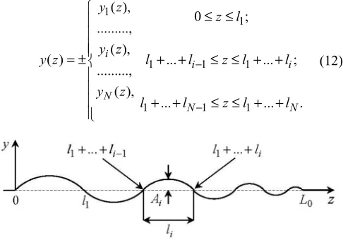
Fig. 2 presents the corresponding model of the normal coronary artery and that of the artery having already a planar pathologically tortuous segment of length L0 (usually, the length of such a segment ranges approximately from 3 mm to 10 mm). In the first case, the artery is represented by an infinite straight rigid pipe, of circular cross-section of diameter D0, in which fluid (blood) flows. The fluid motion
is characterized by the flow rate Q0 (which is so far unknown). In the second case, the artery is modelled by an infinite straight hard-walled pipe having circular cross-section of constant diameter Dw ( Dw=D0−ε ,
0
0<ε/D <<1)2 and a finite planarly tortuous segment. This segment has N arcs (which are its parts between the two neighbouring points of its wall intersection with the dashed line (this line corresponds to the pipe wall location before the appearance of the tortuosity)). Each arc is characterized by height Ai (which is the maximal distance from its wall to the dashed line) and width li (this is the distance between its ends) (i=1,...,N ). The moving fluid in this pipe has the flow rate Qw (which is also so far unknown).
Figure 2. Originally straight and subsequently tortuous segment of a coronary artery.
The considerations and the assumptions used in developing this model are given below.
2.2. The Considerations and the Assumptions
2.2.1. Larger Coronary Artery
Larger coronary artery in a normal state actually is a finite nearly straight slightly taper (in the flow direction) elastic pipe having nearly circular cross-section. However, in this study the artery is modelled by an infinite straight rigid-walled pipe of constant (along its axis) circular cross-sectional shape and area. Such a representation of the artery is mainly for the following two reasons. Firstly, consideration of an infinite pipe (instead of a finite one), with the given typical flow parameter values at infinity, allows one to determine (with satisfactory for cardiologists precision) the flow characteristics of interest in the vessel segment under consideration and not to pay attention to what is upstream and downstream of that segment. Secondly, it is clear that, at the chosen precision of the investigation (see the end of the Introduction and the very beginning of this section), the neglect of both the insignificant deflection of the arterial cross-sectional shape from the circular one and the slight arterial taperedness will not have a principal influence on the results and the conclusions of this study. As for the arterial wall compliance and its influence on the inner blood flow, as well as the arterial fastening in the ambient medium and the
ambient medium effects, etc., all of them (together with those noted above) are indirectly taken account of in the model (via the blood velocity which is found experimentally from the corresponding coronarographies containing all the information of interest (see Section 6)).
2.2.2. Pathologically Tortuous Arterial Segment
The appearance of pathological tortuosity in some arterial segment is accompanied by its non-significant narrowing2. This is taken into account in the model shown in Fig. 2 via the diameter Dw, which is slightly smaller than the diameter
0
D . As for the planar geometry of the tortuosity, this is only a first approximation in its modelling.
2.2.3. Blood
from the above noted ones, as well as the other features of blood rheology (such as dependence of the blood mass density and viscosity on the body temperature, etc.), they are indirectly taken account of in the developed model. Again, it is made via the blood flow velocity (see Subsection 2.1).
2.2.4. Flow
Real blood flow is pulsatile, having the pulsation frequency and time period of the order of 1Hz and 1s, respectively. However, in the model, one actually restricts oneself to the consideration of quasi-steady flow, whose integral characteristics coicide with the corresponding characteristics of real blood flow observable in patients. Also, the model flow is assumed to be a laminar. The former restriction is explained by the fact that at this stage only the blood volume reaching a myocardium during the heartbeat period is of urgent interest rather than how that volume varies over the period4. As for the later assumption, it reflects the reality quite well, because usually real blood flow is laminar. If nevertheless it is disturbed (or even becomes turbulent) in some vessel segment, then, due to the absence of the corresponding perturbation sources and the permanent influence of viscous forces on the flow behind the segment, the flow disturbances (turbulisation) vanish rather fast, and the flow redevelops back to the state upstream of the segment [19-23]. (Here attention should be also paid to the following two circumstances. Firstly, due to the accuracy accepted in this study (see above), the quasi-steady and laminar approximations to real blood flow are not very principal for the results and the conclusions of this study. This is due to that (as one can see in Section 6) (i) the time intervals (over which a Roentgen-contrast fluid passes through the coronary artery segments of concern) will be significantly smaller than the time scale of the problem under consideration (i.e., the heartbeat period), which makes the flow variation over the intervals not a very significant factor; (ii) the solution to the problem will be obtained in terms of the flow characteristics averaged in the appropriate manner, which significantly reduces the difference between the model and real flows. And secondly, the real blood flow character and regime are nevertheless taken account of indirectly in the model shown in Fig. 2. As in the cases of the other constructive elements of the model (see above), it is made via the blood flow velocity, which is found experimentally from the appropriate coronarographies.)
3. Solution to the Problem
3.1. General Relationships
Since among all the blood flow dynamical characteristics the most important for normal functioning of the myocardium are the blood flow rate and cross-sectionally averaged axial velocity, these characterisitcs are paid the
4 The blood volume reaching a myocardium during one heartbeat period is much more important for normal functioning of the myocardium compared with the way in which that volume reaches a myocardium over the noted period.
main attention to in this study. If the blood volume passing across some vessel cross-section, A z( ), over a small time interval ∆t is denoted by∆V z( ) (where
z
is the axis chosen in Fig. 2), then the blood flow rate in that section, Q z( ), is found as the ratio of ∆V and ∆t, viz./
Q= ∆V ∆t. (1)
If one takes into account that the volume ∆V is found as the integral of the local axial blood flow velovity, u, over the section
A
, viz.d
A
V u t A
∆ =∫∫ ∆ ,
the magnitude
Q
in (1) can be represented by the following integrald
A
Q=∫∫u A. (2)
On the other hand, the multiplication and division of the right part of (2) by A (where A is the area of the section
A
) and taking account of the fact that the ratio of the integral and A is the cross-sectionally averaged (mean) axial blood flow velocity, U, in the sectionA
, viz.1 d
A
U u A
A
= ∫∫ (3)
allows one to represent the flow rate
Q
in a simplified form, viz.Q=U A . (4)
For the pipes depicted in Fig. 2, (2) and (4) are rewritten as follows
0
0 0 0
2 0 0
d ,
/ 4,
A
u A
Q
U πD
∫∫
=
(5)
w
w w w
2
w w
d ,
/ 4.
A
u A
Q
U πD
∫∫
=
(6)
Here, in accordance with (3),
0
0 2 0 0
0
4
d
A
U u A
D π
= ∫∫ ,
w
w 2 w w
w
4
d
A
U u A
D π
= ∫∫ , (7)
and hereinafter the indices “0” and “w” indicate the normal and tortuous vessel, respectively.
investigation, and then, based on the expressions
2 2
0 w w
0 w 0
0 0
1 4
D U D
Q Q Q U
U D
π
∆ = − = −
,
0 w
U U U
∆ = − , (8)
2
w w
0 0 0
100% 1 100%
Q
U D
Q
Q U D
δ =∆ × = − ×
,
w
0 0
100% 1 100%
U
U U
U U
δ =∆ × = − ×
, (9)
find the absolute (8) and relative (9) changes in these flow characteristics, which are caused by the appearance of the noted tortuosity. However, as one can see from the analysis of (5)-(9), these mathematical operations can be only made under the availability of a complete and reliable information about the corresponding local (i.e., u0, uw) and/or mean (i.e., U0, Uw) axial blood flow velocities.
This information can be obtained by the two methods. The forst of them is based on direct numerical modelling of the flow in the arterial segment under consideration, with taking account of all the rheological features of blood, properties of the arterial wall and its fastening, the blood-wall interaction, etc. It allows one to find rather accurately the velocities u0 and uw, and hence, the magnitudes Q0, Qw and U0, Uw. However, this approach is associated with significant time and financial expenses, which is undesirable (because patients prefer to have fast and cheap diagnostics, whereas cardiologists need to make fast (or even immediate) and correct decision about the patient state). Therefore, so far it is unacceptable.
The second method (its description is given in Subsection 3.2) is in approximate experimental determination of the mean flow velocities U0 and Uw (proceed from the appropriate data obtained from the corresponding coronarographies), with subsequent computation of the flow rates Q0 and Qw based on the lower expressions in (5) and (6). Herewith the blood rheology, the arterial wall properties and the artery fastening in the ambient medium, as well as the blood-wall interaction, etc are taken account of automatically from the corresponding coronarographies. This approach does not need much time (maximum a couple of hours for making a decision) and financial expenses, its precision is satisfactory for cardiologists, and hence, for the moment it is more acceptable for them compared to the first method.
Proceed from the just-noted, further in this paper the second approach is chosen to find the velocities U0 and Uw, and consequently, the flow rates Q0 and Qw, as well as the absolute and relative changes in these flow characteristics.
3.2. A Method to Find U and 0 U w
Before proceeding to description of this method, let us pay
our attention to one important physical feature of mathematically equivalent expressions (2) and (4), as well as the consequences resulting from that feature. The matter is that the formal transition from (2) to (4) on the basis of (3) means not only the transition from the local, u, to averaged,
U , axial flow velocity but also (that is much more important) the transition from the consideration of real to the averaged, in the appropriate manner, flow (because the averaged flow velocity is a velocity of the appropriately averaged flow). Further, in a cross-sectionally averaged (quasi-steady) laminar flow (such a flow is actually observed by cardiologists when studyng coronarographies (see also Subsection 2.2.4)) the velocities of all fluid particles are equal vectors (Fig. 3), and their trajectories, therefore, are identical curves which have the same length [24]. Apart from the others, it means that in such a flow in vessel (i) the trajectories of all fluid particles are like the vessel axis; (ii) the distance
L
covered by the particles during some time ∆tis equal to the length of the corresponding axial segment; (iii) the fluid particle velocity (i.e., the mean axial flow velocity,
U ) is determined as the ratio of the distance
L
and the timet
∆ , viz.
/
U =L ∆t. (10)
Figure 3. Schematic profiles of u and U in a laminar pipe flow.
The above considerations allow one to determine approximately the velocities U0 and Uw based on the appropriate data obtained from the corresponding coronarography (CAG) only and formula (10). The corresponding general procedure of finding the noted velocities reduces to the following three main steps, viz. (i) determination of the distance
L
covered by the Roentgen-contrast fluid front together with blood in the arterial segment under investigation proceed from the appropriate data taken from the corresponding CAG; (ii) finding the time interval ∆t, during which the above-noted front passes the distanceL
, based on the number of corresponding picture areas of the investigated CAG and the time duration of one picture area; (iii) calculation of the blood flow velocity of concern on the basis of the above data forL
and ∆t, as well as formula (10).Originally normal arterial segment. The length L0 of the originally normal arterial segment (Fig. 2) and the time T0, during which the front of a Roentgen-contrast fluid passes through the segment (i.e., covers the distance L0), are found from the chosen CAG by direct measuring and counting (proceed from the number of the corresponding picture areas and the time duration of one picture area), respectively. Then the velocity U0 is calculated from the ratio
0 0/ 0
U =L T . (11)
Pathologically tortuous arterial segment. The distance
w
L covered by the Roentgen-contrast fluid front, when it passes through the tortuous arterial segment (Figs. 1, 2), is equal to the length of the segment axis (the corresponding arguments are given before (10)). Since the axis has the shape of an irregular sinusoid, it is logically to approximate the segment axis by such a sinusoid (Fig. 4), viz.
1( ),
..., ( ), ( ) ..., ( ), i N y z y z y z y z = ± 1
1 1 1
1 1 1
0 ; ... ... ; ... ... . i i N N z l
l l z l l
l l z l l
− − ≤ ≤ + + ≤ ≤ + + + + ≤ ≤ + + (12)
Figure 4. The tortuous segment axis approximated by an irregular sinusoid.
Here y zi( ) (i=1,...,N ) are ordinary sine functions in the indicated domains, viz.
1( ) 1sin( / )1
y z = A πz l
,
1
1 1
( ) ( 1)i sin( ( ... ) / )
i i i i
y z = − − A π z− − −l l− l , (13)
1
1 1
( ) ( 1)N sin( ( ... ) / )
N N N N
y z = − − A π z− − −l l − l ,
which approximate the axes of the corresponding arcs, the magnitudes Ai and li are their heights and widths, respectively, (they are identical to those shown in Fig. 2) and are measured directly from the corresponding coronarogramm, and the plus-minus signs indicate the cases when the first arc is either above or below the
z
-axis, respectively.In such a situation, the distance Lw can obviously be found as the length of the curve (12), (13), viz.
w 1 N i i L L =
=∑ , (14)
where 1 1 1 2 ... ... d 1 d d i i l l i i l l y L z z − + + + + = ∫ + = 2 /2 2 0
2i 1 cos d
l i i i A z z l l π π = ∫ +
is the length of the i -th axial arc. This length, after introducing the following non-dimensional variables
/ i i
z l x
π = , Aiπ/li =ai,
k
i=
a
i/ 1
+
a
i2 , ki <1,can be rewritten in terms of the total elliptic integral of second kind, E k
( )
i , as [25]( )
22 i 1
i i i
l
L a E k
π
= + ,
( )
/2 2 20
1 sin d
i i i i
E k =π∫ −k x x . (15)
The availability of the distance (14) and the time Tw
needed for the front of a Roentgen-contrast fluid to cover that distance (Twis found from the investigated CAG by direct counting the number of the corresponding picture areas and subsequent multiplying that number by the time duration of one picture area) allows one to find the velocity Uw as the ratio of Lw and Tw, viz.
w w/ w
U =L T . (16)
4. The Method
The considerations presented, as well as the results and the relationships obtained in Sections 2 and 3 allow one to suggest the following approximate method to find the hemodynamic significance of a pathological tortuosity of larger coronary arteries in patients with cardiac ischemia and cardiac syndrome X for the case of planar tortuosity.
(a) When the patient exhibits the common symptoms of cardiac ischemia (such as chest pain (typically on the left side of the body), neck or jaw pain, shoulder or arm pain, a fast heartbeat, shortness of breath when he/she is physically active, extreme fatigue and sweat secretion, etc. [1, 2, 15]), his/her coronary angiography (CAG) is carried out.
(b) If the obtained CAG does not exhibit stenoses in coronary arteries and at least one coronary artery has a segment with a severe pathological tortuosity, then the segment cross-sectional diameter, Dw, as well as the height,
i
A , and the width, li, of each segment arc (i=1,...,N; Fig. 2) are determined from the CAG by direct measuring.
(d) Based on (14) and (15), as well as the tables of the total elliptic integral of second kind [25], the axis length Lw (i.e., the distance covered by the Roentgen-contrast fluid front when moving together with blood through the segment) is found.
(e) The time Tw, needed for the front to cover the distance
w
L , is determined from the investigated CAG as the product of the number of the corresponding picture areas and the time duration of one picture area.
(f) The mean axial blood flow velocity, Uw , in the investigated tortuous segment is found from (16).
(g) As the originally normal coronary artery (i.e., the investigated artery before the appearance of the totuosity in it) an artery without pathological tortuosity is chosen in the
same CAG5. Its cross-sectional dimension, D0, shoud be slightly larger than the diameter Dw (i.e., D0=Dw+ε ,
w
0<ε/D <<1)2. In this artery, a straight segment (or, in case of absence of a straight segment, a segment whose shape is maximally close to the straight one) is further considered, whose length, L( )0s , is close to the axial dimension of the investigated tortuous segment, L0 (i.e., L( )0s ≈L0, Fig. 2)6.
(h) Based on the number of the corresponding picture areas and the time duration of one picture area (which are taken from the used CAG), the time T0, needed for the front of a Roentgen-contrast fluid to cover the chosen straight segment of the conditionally normal coronary artery (i.e., the distance L( )0s ), is found as the product of the above number and the time duration.
(i) The mean axial blood flow velocity in this straight arterial segment, U0, is determined on the basis of (11), where L0 is replaced byL( )0s .
(j) Based on the above data and the lower expressions in (5) and (6), the blood flow rates in the conditionally normal,
0
Q , and pathologically tortuous, Qw, arterial segments are calculated.
5 Such a choice of an originally normal coronary artery is for the following two reasons. Firstly, it is practically impossible to have a previously recorded coronarography of the patient, when the investigated artery did not have the pathological tortuosity (because usually the patient comes to a cardiologist only when he/she already has some problems with the heart). Secondly, the choice of the artery in the same CAG provides making the comparative analysis of the corresponding data for the originally normal and subsequently pathologically tortuous artery under the other equal conditions.
6 This is only a desirable condition. If this condition cannot be realized, it will not result in significant errors in finding the flow characteristics of interest, and hence, significat errors in the results of this study and the subsequent conclusions made by cardiologists. It is explained by the fact that the velocity U0 of the cross-sectionally averaged quasi-steady laminar flow in the artery is a constant value (see the considerations regarding the flow given in Sections 2 and 3.2, as
well as Fig. 3). Therefore, the ratio of the distance L( )0s (or L0), covered by that flow in the artery, to the corresponding time T0( )s (or 0T ) is always equal to the velocity U0 (i.e., L( )0s /T0( )s =U0, L0/T0 =U0).
(k) Based on (8) and (9), the absolute and relative changes in the corresponding blood flow characteristics in the coronary artery under investigation, which are caused by the appearance of the pathological tortuosity in it, are found.
(l) The hemodynamic significance of those changes is determined, the changes being considered to be hemodynamically significant when the relative blood flow rate loss, δQ , is not less than the corresponding critical value, δQcr =40% (i.e., δQ ≥δQcr). In the opposite case (i.e., when δQ <δQcr ) the changes are hemodynamically insignificant (the value δQcr =40% corresponds to the 25% drop in the blood pressure in vessel due to a stenosis, which is hemodynamically significant according to the FFR method3).
5. Experimental Verification of the
Method
5.1. Experimental System
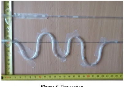
In order to verify the above-described method before its application to appropriate patients, it has been tested in a laboratory experiment. For this purpose, a suitable experimental system has been developed. A schematic of this system and its test section is shown in Figs. 5 and 6, respectively. Here the basic elements are: (i) a couple of the upper supply and a couple of the lower collection identical reservoirs; (ii) two identical silicone pipes, of inner diameter
3
D= mm, representing an originally healthy and subsequently tortuous larger coronary artery (see below the explanation of how the pipe shape was fixed); (iii) measuring reels to measure the pipes’ geomethical parameters of interest; (iv) needles (for dye injection) flush-mounted into the pipe wall upstream of the test section; (v) a videocamera to record the dye motion in the pipes; (vi) transparent glue ribbon to fix the pipe shape of interest; (vii) electronic balances to determine the fluid volume, ∆V , accumulated in the collection reservoir during the period of data acquisition,
τ
, based on the formula/
V m ρ
∆ = ∆ (17)
Figure 5. Schematic of experimental system: 1 – supply reservoir; 2 – silicone pipe; 3 – collection reservoir; 4 - electronic balance; 5 – needle for dye injection; 6 – test section; 7 – table.
Figure 6. Test section.
The working medium was water at an indoor temperature (the considerations used in developing the test section were like those given in Section 2 and in [20-22]).
5.2. Operation of the System
The experimental system was operated in the following way. The upper and lower tanks were joined by the pipes (one pipe per one set of the upper and lower tanks). One pipe was straight and represented an originally healthy coronary artery. Another one had a plane tortuous segment, with all the adjusted geometrical parameters of concern (due to pipe flattening, that took place at the tortuosty apices at some ratios of the arcs’ heights and widths, Ai/li, those ratios were not considered in the experiment). It simulated a tortuous coronary artery. Due to the same levels of water in the corresponding reservoirs, a controlled flow with identical pressure gradients was created in each pipe. A similarity in the flow Reynolds number, Re, (based on the mean axial flow velocity in vessel and the inner vessel diameter) between the experimental flow and real blood flow observable in the appropriate coronary arteries in the patients was held herewith (for all the patients used in this study (see Section 6), the number Re did not exceed 1800, that indicated that the flow in the coronary arteries of interest and the experimental flow were always laminar [20-22]. Mild dye injection into the pipes via the needles situated immediately upstream of the test section allowed one to visualize the flows and make their videorecords.
For these experimental flows, their mean axial velocities,
0
U and Uw, and the coresponding flow rates, Q0 and Qw, were determined on the basis of the method described in Section 4. Then these data were compared with the
corresponding reference data. After that, proceed from the results of such a comparison and the corresponding discussions with the cardiologists, a conclusion concerning the applicability of the method to appropriate patients was made.
The reference data were obtained on the basis of the corresponding measurements. More specifically, initially the water masses, passed simultaneously from the straight, ∆m0, and tortuous, ∆mw , pipes to the appropriate collection reservoirs during the period
τ
, were measured by means of the electronic balances. It allowed one to find the flow rates in the pipes, Q0 and Qw, from (1) and (17), viz.0 0/ 0/ ( )
Q = ∆V τ= ∆m ρτ , Qw = ∆Vw/τ= ∆mw/ (ρτ)
(here
∆
V
0 and ∆Vw are the corresponding water volumes accumulated in the collection reservoirs during the timeτ
7). Then the found data for Q0 and Qw and the lower expressions in (5), (6) were used to compute the corresponding velocities U0 and Uw, viz.82 0 0/ ( / 4)
U =Q πD , Uw =Qw/ (πD2/ 4).
5.3. Experimental Results
Some typical results of such a comparison, obtained for the pipes’ configurations shown in Fig. 6, are presented below. Here the axial dimension of the tortuous segment, L0, and the number of its arcs, N, were chosen to be 200mm and 5, respectively, and the values of the arcs’ heights, Ai, and
widths, li, (i=1,...,N ) were as those given in Table 1. With these magnitudes available and in accordance with the method described in Section 4, the tortuous segment axis was then approximated by the irregular sinusoid (12), (13). Further application of (14) and (15), as well as the use of the above magnitudes and the tables of the total elliptic integral of second kind [25] allowed one to find both the lengths Li
of the axial arcs (Table 1) and the length Lw of the tortuous segment axis (i.e., the distance covered by the dye when it moved through the segment), viz. Lw =375mm.
7 In making these measurements, the period τ was identical for both pipes, although in obtaining the magnitudes U0, Q0 and Uw, Qw on the basis of
the method, the corresponding periods T0 and Tw were different (because
0 w
L <L , U0>Uw and hence, T0<Tw ). However, this fact did not influence significantly the obtained results of the comparison and the subsequent conclusions made. (To get the noticeable difference between the masses ∆m0
and ∆mw and depending on the situation, the period τranged from 1s to 10s, with steps of 1s; during this time the difference between the levels of water in upper and lower reservoirs changed negligibly (less than 1% of its relative value); in such a situation, the experimental flow could thus be considered quasi-steady). 8 For technical reasons, in the experiment it was impossible to reduce noticeably the cross-sectional area of the tortuous pipe to get the desired condition
w 0
Table 1. Values (in mm) of the tortuosity parameters in Fig. 6.
i 1 2 3 4 N=5
Ai 37 19 34 10 49
li 48 31 33 27 61
Li 92 51 77 35 120
The availability of the distances L0 and Lw, as well as the corresponding time intervals T0=0.44 s and Tw=1.04 s (found by the way indicated in the method) gave one (on the basis of (11) and (16)) the values of the mean axial flow velocities in the straight, U0 , and tortuous, Uw , pipe segments, viz.
0 455
U = mm/s, Uw=361mm/s. (18)
Then the magnitudes (18) allowed one to determine (proceed from the lower expressions in (5) and (6)) the corresponding flow rates Q0 and Qw, viz.
3 0 3.215 10
Q = × − l3/s, 3
w 2.55 10
Q = × − l3/s, (19)
and the corresponding absolute and relative losses in these flow characteristics, viz.
94
U
∆ = mm/s, ∆ =Q 0.665 10× −3l3
/s,
20.66
U
δ = %,
δ
Q =20.68%, (20) which are caused by the appearance of the tortuosity.The comparative analysis of the values (18)-(20) with the corresponding reference data, viz.
0 473
U = mm/s, Uw=371mm/s,
3 0 3.341 10
Q = × − l3/s, 3
w 2.621 10
Q = × − l3/s,
102
U
∆ = mm/s, ∆ =Q 0.72 10× −3 l3/s,
21.56
U
δ = %,
δ
Q=21.55%(found in the manner described above) showed rather good agreement between them. Also, this agreement was acceptable for the cardiolgists.
Similar results of the comparison (i.e., within 10% of the corresponding relative differences) have also been obtained for all the other tortuosity configurations used in this experiment. From this and the corresponding discussions with the cardiologists, one has come to the conclusion that the method described in Section 4 gave one the results which were acceptable for cardiologists and hence, it could be applied to appropriate patients.
6. Clinical Application of the Method
After the successful laboratory verification of the method it was further used in the Saint Catherine’s cardiological clinic (Odessa, Ukraine). In the clinic, among 2815 investigated patients with the common symptoms of cardiac ischemia (MI), 272 ones (9.66%) had the cardiac syndrome
X, and in 231 patients (84.93%) of the latest ones a severe pathological tortuosity of larger coronary arteries was clearly observed. The number of arcs in their tortuous arteries ranged from 2 to 14 (i.e., 2≤ ≤N 14). In order to determine the hemodynamic significance of the tortuosity in these patients, the above-noted method was applied. Below an example of application of the method to the patient, whose coronarogram is shown in Fig. 1 (this is a standard left skew cranial projection), is demonstrated.
In this patient, by means of making appropriate physical exercises, the common symptoms of MI were detected, and accordingly, the coronarography (CAG) was carried out (item (a) of the method, see Section 4). In this CAG, stenoses were absent. However, one larger coronary artery, having a segment with a severe pathological tortuosity, was observed (the artery is denoted by number 1 in Fig. 1; this is the anterior interventricular branch of the LCA, which is often affected by such involvements). This segment had 9 arcs (i.e.,
9
N= ), its cross-sectional diameter, Dw, found from the CAG by direct measurement, was equal to 1.7mm, and the values of the heights, Ai, and the widths, li , of all its arcs, also found from the CAG by direct measuremnt, are given in Table 2 (item (b) of the method).
Table 2. Values (in mm) of the geometrical parameters of the tortuous arterial segment chosen in Fig. 1.
i 1 2 3 4 5 6 7 8 N=9
Ai 2.8 2.8 2.9 2.8 2.9 2.0 1.8 1.1 1.6
li 6.7 6.8 5.6 4.3 4.6 3.5 5.0 2.6 2.5
Li 9.03 9.08 8.33 7.31 7.65 5.52 6.34 3.51 4.21
The availability of values of Ai and li allows one (in accordance with items (c) and (d) of the method) (i) to approximate the axis of the tortuos segment by the irregular sinusoid (12), (13); (ii) to determine the lengths Li (Table 2) of all the axial arcs based on (15) and the tables of the total elliptic integral of second kind [25]; (iii) to find the distance
w
L , which is covered by blood when moving through the segment, proceed from relationship (14), viz.
9 w
1
60.98
i i
L L
=
= ∑ = mm.
Then the found distance Lw and the time Tw (Tw =0.6 s)9, which is needed for blood to pass the distance, allow one to determine the mean axial blood flow velocity, Uw, in the discussed segment proceed from (16), viz.
w 101.63 U = mm/s
(items (e) and (f) of the method).
Further, in accordance with item (g) of the method, the artery without pathological tortuosity, having almost straight
segment of length L( )0s =19.5mm, is chosen in the same CAG as the originally normal coronary artery (it is denoted by number 2 in Fig. 1; this is the envelope branch of the LCA in the proximal-middle segment in the standard straight caudal projection; for the convenience of making the investigation, it was re-projected by the cardiologists to the standard left skew cranial projection shown in Fig. 1)10. The cross-sectional diameter of this segment, D0, is equal to 1.8mm (D0>Dw).
The chosen segment is covered by a Roentgen-contrast fluid during passing only one picture area. Since the time duration of one picture area is9 0.1s, the time T0, required for the fluid to pass the distance L( )0s , is equal to 0.1s (item (h) of the method), and hence, in accordance with item (i) of the method, the mean axial flow velocity in the segment is equal to 195mm/s (i.e., U0=195mm/s).
The availability of the velocities U0 and Uw, as well as the diameters D0 and Dw allows one
(i) to determine the blood flow rates in the originally normal, Q0, and subsequently pathologically tortuous, Qw, segment of the investigated coronary artery based on the lower expressions in (5) and (6) (item (j) of the method), viz.
3 0 0.49596 10
Q = × − l3/s, Qw=0.23056 10× −3l3/s;
(ii) to find the absolute and relative changes both in the mean axial flow velocity and the flow rate in this artery proceed from (8) and (9), which are caused by the appearance of the pathological tortuosity in the artery (item (k) of the method), viz.
93.37
U
∆ = mm/s, ∆ =Q 0.2654 10× −3 l3/s,
47.88%
U
δ = , δQ =53.51%.
Then the comparison of the obtained value of the relative blood flow rate loss, δQ =53.51%, with the corresponding critical one, δQcr =40% , shows that these changes are hemodynamically significant (item (l) of the method), viz.
cr
Q Q
δ >δ
.
In general, the application of the method to the above-mentioned 231 patients with a severe pathological tortuosity of larger coronary arteries has shown that in 141 of them (61.04%) the tortuosity was hemodynamically significant, whereas the other 90 patients (38.96%) had the hemodynamically insignificant arterial pathology.
10 One can see that the length L( )0s is less than the axial dimesion of the
investigated tortuous segment, 41.6
9 0
1
L li
i
= =
=
∑ mm. However, according to
item (g) of the method and footnote 6, it is not principal for the resuls and conclusions of this study.
Further, among the patents with 2 or 3 arterial arcs nobody had hemodynamically significant tortuosity. The significance of hemodynamically significant tortuosities having more than 3 arcs generally increased as the number of arcs, N , increased. However, the situations were observed when pathologically tortuous arterial segments with the bigger number of arcs were hemodynamically less significant compared to the segments having the smaller number of arcs. It is explained by the corresponding dependence of the tortuous segment resistance to blood motion, Rts, on the heights, Ai , and the widths, li , of the segment arcs (i=1,...,N ), the ratios Ai/li, etc. However, obtaining of a functional dependence of Rts on the noted parameters requires carrying out extensive appropriate investigations.
7. Conclusion
Based on the analysis of coronarographies of patients with cardiac ischemia and cardiac syndrome X, an approximate method has been developed to allow cardiologists to find (with satisfactory precision and speed) both changes in the blood flow rate in larger coronary arteries, caused by the appearance of their planar pathological tortuosity, and a hemodynamic significance of those changes based on the data taken from the appropriate coronarographies only. This method is based on replacement of real blood flows in the originally healthy and subsequently pathologically tortuous artery with the corresponding cross-sectionally averaged ones, and subsequent calculation of the blood flow characteristics of interest in terms of the corresponding averaged flow characteristics. The method allows one not to take account of a number of identical factors for the originally healthy and subsequently pathologically tortuous segment of the coronary artery under investigation (such as arterial pressure, the number of heartbeats, the inflow rate in the segment, mass density, viscosity and temperature of the blood, the physical and geometrical characteristics of the arterial wall, etc.). In addition, it gives one the possibility to determine the blood flow parameters of concern at any time after carrying out a coronarography, is not associated with solving complicated technical problems, and does not require special facility to be used, special professional training and significant expences.
Nomenclature
i
A height of the i-th arc, mm
CA coronary artery CAG coronarography
D
inner diameter of pipe, mm0
D diameter of a normal vessel, mm
w
D diameter of a tortuous segment, mm LCA left coronary artery
0
L axial dimension of a tortuous segment, mm
( ) 0
s
L length of the straight segment of a conditionally
i
L length of the i-th arc, mm
w
L length of a tortuous segment, mm
i
l width of the i-th arc, mm
MI myocardial ischemia
N the number of arcs
Q
flow rate, l3/s0
Q flow rate in a normal vessel, l3/s
w
Q flow rate in a tortuous vessel, l3/s RCA right coronary artery
0
T time needed for blood to pass the straight segment
of a normal artery, s
w
T time needed for blood to pass the tortuous arterial
segment, s
U mean axial flow velocity, mm/s
0
U mean axial flow velocity in a normal vessel, mm/s
w
U mean axial flow velocity in a tortuous vessel, mm/s
Acknowledgments
The author expresses gratitude to the Chief Doctor of the Saint Catherine’s cardiological clinic (Odessa, Ukraine) Dr. D. M. Sebov for his stimulation of and promotion to making the research described in this paper, as well as for the corresponding materials provided and the useful comments given by him in discussing this work. Thanks are also expressed to all personnel of the clinic who directly or indirectly helped to carry out this research. A major part of the financial expenses related to the research was covered by the clinic.
References
[1] Wikipedia, last modified September 30, 2012, http://en.wikipedia.org/wiki.
[2] “Your Coronary Arteries”, Cleveland Clinic, http://my.clevelandclinic.org/services/heart/heart-blood-vessels/coronary-arteries.
[3] A. Aldrovandi, et al., “Evaluation of coronary atherosclerosis by multislice computed tomography in patients with acute myocardial infarction and without significant coronary artery stenosis: a comparative study with quantitative coronary angiography,” Circulation: Cardiovascular Imaging, vol. 1, pp. 205-211, 2008.
[4] A. Aldrovandi, et. al, “Computed tomography coronary angiography in patients with acute myocardial infarction without significant coronary stenosis,” Circulation, vol. 126, pp. 3000-3007, 2012.
[5] F. Crea, and G. A. Lanza, “Angina pectoris and normal coronary arteries: cardiac syndrome X,” Heart, vol. 90, pp. 457-463, 2004.
[6] S. S Groves, A. C. Jain, B. E. Warden, W. Gharib, and R. J. Beto 2nd., “Severe coronary tortuosity and the relationship to significant coronary artery disease,” West Virginia Medical Journal, vol. 105, pp. 7-14, 2009.
[7] H.-C. Han, “Twisted blood vessels: symptoms, etiology and
biomechanical mechanisms,” J. Vasc. Res., vol. 49, pp. 185– 197, 2012.
[8] W. E. Hart, M. Goldbaum, B. Coˆte´, P. Kube, and M. R. Nelson, “Measurement and classification of retinal vascular tortuosity,” Int. J. Med. Inf., vol. 53, pp. 239–252, 1999. [9] J. C. Kaski, “Pathophysiology and management of patients
with pain and normal coronary arteriograms (cardiac syndrome X),” Circulation, vol. 109, pp. 568-572, 2004. [10] J. C. Kaski, G. Aldama, and J. Cosin-Sales, “Cardiac
syndrome X. Diagnosis, pathogenesis and management,” Am. J. Cardiovasc. Drugs, vol. 4, no. 3, pp. 179-194, 2004. [11] Y. Li, et. al., “Impact of coronary tortuosity on coronary pressure:
numerical simulation study,” PLOS ONE, vol. 7, pp. 1-6, 2012. [12] T. Schubert, et. al., “Dampening of blood-flow pulsatility
along the carotid siphon: does form follow function?,” Am. J. Neuroradioly, vol. 32, pp. 1107–1112, 2011.
[13] P. D. Stein, et al., “Effects of cyclic flection of coronary arteries on progression of atherosclerosis,” Am. J. Cardiology, vol. 73, pp. 431-437, 1994.
[14] E. S. Zegers, B. T. J. Meursing, E. B. Zegers, and A. J. M. Oude Ophuis, “Coronary tortuosity: a long and winding road,” Netherlands Heart J., vol. 15, pp. 191 – 195, 2007.
[15] “Myocardial Ischemia”, Mayoclinic,
http://www.mayoclinic.org/diseases-conditions/myocardial-ischemia/basics/symptoms/con-20035096.
[16] C. Caiati, C. Montaldo, N. Zedda, A. Bina, and S. Iliceto, “New noninvasive method for coronary flow reserve assessment: contrast-enhanced transthoracic second harmonic echo doppler,” Circulation, vol. 99, pp. 771-778, 1999. [17] N. H. J. Pijls, et al., “Measurement of fractional flow reserve
to assess the functional severity of coronary-artery stenosis,” New Eng. J. Med., vol. 334, pp. 1703–1708, 1996.
[18] P. A. L. Tonino, et al., “Fractional flow reserve versus angiography for guiding percutaneous coronary intervention,” New Eng. J. Med., vol. 360, pp. 213–224, 2009.
[19] S. A. Berger, and L. D. Jou, “Flows in stenotic vessels,” Ann. Rev. Fluid Mech., vol. 32, pp. 347-382, 2000.
[20] A. O. Borisyuk, “Experimental study of noise produced by steady flow through a simulated vascular stenosis,” J. Sound Vibr., vol. 256, pp. 475-498, 2002.
[21] A. O. Borisyuk, “Model study of noise field in the human chest due to turbulent flow in a larger blood vessel,” J. Fluids Str., vol. 17, pp. 1095-1110, 2003.
[22] A. O. Borisyuk, “Experimental study of wall pressure fluctuations in rigid and elastic pipes behind an axisymmetric narrowing,” J. Fluids Str., vol. 26, pp. 658-674, 2010. [23] D. F. Young, “Fluid mechanics of arterial stenoses,” ASME J.
Biomech. Eng., vol. 101, pp. 157-175, 1979.
[24] G. K. Batchelor, An Iintroduction to Fluid Dynamics. Cambridge Univ. Press, Cambridge, UK, 1967.