Article
1
Integrated Modeling Approach for the Development
2
of Climate-Informed, Actionable Information
3
David R. Judi 1,*, Cynthia L. Rakowski 1, Scott R. Waichler 1, and Youcan Feng 1
4
1 Pacific Northwest National Laboratory, Richland, WA 99354, U.S.A.
5
* Correspondence: [email protected]
6
7
Abstract: Flooding is a prevalent natural disaster with both short and long-term social, economic,
8
and infrastructure impacts. Changes in intensity and frequency of precipitation (including rain,
9
snow, and rain on snow) events create challenges for the planning and management of resilient
10
infrastructure and communities. While there is general acknowledgement that new infrastructure
11
design should account for future climate change, no clear methods or actionable information is
12
available to community planners and designers to ensure resilient design considering an uncertain
13
climate future. This research used climate projections to drive high-resolution hydrology and flood
14
models to evaluate social, economic, and infrastructure resilience for the Snohomish Watershed,
15
WA, U.S.A. The proposed model chain has been calibrated and validated. Based on the established
16
model chain, the peaks of precipitation and streamflows were found to shift from spring and
17
summer to earlier winter season. The nonstationarity of peak discharges was discovered with more
18
frequent and severe flood risks projected. The peak discharges were also projected to decrease for a
19
certain period in the near future, which might be due to the reduced rain-on-snow events. This
20
research was expected to provide a clear method for the incorporation of climate science in flood
21
resilience analysis and to also provide actionable information relative to the frequency and intensity
22
of future precipitation events.
23
Keywords: climate projections; integrated modeling; flood modeling; nonstationarity
24
25
1. Introduction
26
Extreme flooding has been observed to become more prevalent and is expected to worsen with
27
a changing climate considering the potential for increased precipitation and rain-on-snow events in
28
regions of the United States[1]. Traditional approaches to designing flood mitigation strategies have
29
assumed a stationary climate, but it is increasingly important to consider changes in magnitude and
30
frequency extreme events and include future climate scenarios in design [2].
31
In many cases, the standards currently used in flood mitigation design using stationary climate
32
assumptions (e.g., historical 100-year return period) are no longer sufficiently conservative
33
assumptions [1]. In recognition of this, there have been recent changes in design standards and
34
floodplain management policy which call for the “consideration” of possible changes induced by
35
climate change [3]. For example, in 2015 a U.S. Presidential Executive Order (13690) mandated
36
changes in the federal flood risk management standard. This order gave agencies the flexibility to
37
either 1) use data and methods informed by best-available, actionable climate science, 2) build two
38
feet above the 100-year flood elevation for standard projects or three feet above for critical buildings,
39
or 3) build to the 500-year flood elevation. Specific guidance on appropriate methods informed by
40
best-available, actionable climate science is not available. Moreover, blindly raising infrastructure by
41
a defined, uniform threshold does not adequately consider risk and may result in either over or under
42
designed mitigation. Approaches that explicitly consider future climate scenarios are needed in order
43
to adequately understand flood risk and develop actionable, climate-informed information at a local
44
scale.
45
One of the primary challenges in developing local-scale, actionable information for future flood
46
risk is related to the temporal and spatial scales of available climate information. To translate climate
47
projections into local-scale flood prediction, multi-modal approaches connecting general circulation
48
models (GCMs), downscaling methods, hydrological modeling, and consequence analysis present an
49
approach to overcome temporal and spatial resolution challenges [4, 5]. In a multi-model, multi-scale
50
approach, a GCM depicts climate variables at a global scale typically with a spatial resolution of
51
multiple degrees and a monthly temporal scale. These spatial and temporal scales are very coarse
52
compared to that of the watershed-scale hydrological processes [6] and therefore inadequate to use
53
alone in understanding the impacts of climate on flood risk management. To represent
watershed-54
scale processes, Regional Climate Models (RCM) dynamically downscaled to a specific region can be
55
developed by utilizing GCM as boundary conditions for higher resolution, regional climate
56
simulations. This approach in developing RCMs parameterizes physical atmospheric processes and
57
accounts orographic effects and mesoscale processes [7, 8].
58
GCMs can also be downscaled through statistical approaches are based on relationships in
large-59
scale climate and regional characteristics identified from observational data [6]. Because these
60
approaches do not have a significant computational burden, they are often the method of choice for
61
downscaling. The method of “change factors”, also known as the perturbation or the delta-change
62
method, is a simple example of statistical downscaling, which applies the difference in GCM
63
projections between the control and future periods to match the baseline observations [8]. Due to its
64
simplicity, this method is widely used by hydrologists [9, 10]. Another simple statistical method is
65
bias correction, which defines a transfer function for GCM/RCM outputs for the control period to
66
match certain statistical properties of the observations [11]. These simple statistical downscaling
67
approaches have a number of caveats, including assuming a stationary bias through time and a
68
constant spatial pattern of climate [8, 11]. To overcome limitations of both dynamical and statistical
69
downscaling methods, statistical-dynamical processes can be used to further remove inherent bias
70
[12].
71
At the watershed scale, hydrologic models ingest climatic variables such as temperature,
72
precipitation, and humidity derived from downscaled GCMs/RCMs to simulate hydrologic processes
73
and ultimately provide a continuous estimate of river discharges. Calibration of hydrologic models
74
is important in order to reduce the uncertainty in the flow estimates, especially for watersheds
75
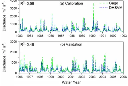
sensitive to pronounced seasonal changes (e.g., rain and snow interactions) [13-15]. Statistical
76
distributions of extreme river discharge events can be developed using the continuous estimates of
77
river discharge [16].
78
To develop actionable flood risk information, thresholds from the statistical distribution of river
79
flows can be developed and used to drive high-resolution flood extent estimation. Various
80
approaches exist to estimate flood extent, including empirical, hydrodynamic, and
non-physics-81
based models [17], but is an essential component in assessing infrastructure exposure to floods and
82
subsequent damage estimates. Ensembles of flood extents and associated damage estimates derived
83
from sampling the statistical river flow distribution are foundational to robust probabilistic risk [18].
84
The objective of this research is to develop an end-to-end, multi-scale, multi-model framework
85
to effectively integrate GCM/RCM, hydrology, and flood risk to develop local-scale, actionable
86
information to be used in flood management. These tools will provide a means to develop mitigation
87
and adaptation strategies to ensure resilient designs of communities and critical infrastructure
88
systems. The achieved actionable information will help local stakeholders (including policy makers,
89
planners, and engineers) understand vulnerabilities and consequences related to the nonstationarity
90
of precipitation events.
91
2. Method
92
To overcome spatial and temporal resolution challenges and incorporate climate nonstationarity
93
into flood risk management, a multi-scale, multi-model flood risk framework has been developed
94
(Figure 1). This framework is intended to provide a means to develop quantifiable and actionable
95
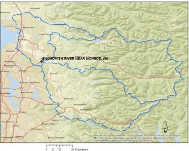
The framework is presented in the context of a case study based on the Snohomish River Basin
97
located near Monroe, WA (Figure 2Error! Reference source not found.). This river basin is of
98
particular interest for this case study because of the river peak flows sensitive to rain, snow, and
rain-99
on-snow events. The basin has frequent fluvial flooding, with overtopping expected to happen every
100
2 to 5 years [19]. The Snohomish River Basin belongs to the U.S. Pacific Northwest region, which was
101
projected to experience the temporal and spatial changes in precipitation, with possible shifts of flood
102
and low flow extremes [20].
103
104
Figure 1. Integrated multi-scale, multi-model framework for flood risk estimation
105
106
Figure 2. The Snohomish watershed (blue lines) and the location of the USGS gauge near Monroe, WA.
107
2.1. Climate Modeling and Downscaling
109
Existing climate datasets from the Platform for Regional Integrated Modeling and Analysis
110
(PRIMA) were extracted for the Snohomish basin [21, 22], where the GCM output was downscaled
111
using the Weather Research and Forecasting (WRF) model [23] with specific emphasis on the Pacific
112
Northwest. These dynamically downscaled climate simulations were then bias corrected to match
113
the North American Land Data Assimilation (NLDAS-2) monthly data [24] as mentioned in Hejazi et
114
al [25] using the Bias-Correction Spatial Disaggregation (BCSD) method described by Wood et al [5].
115
Bias correction was applied to precipitation and temperature, respectively. For temperature, the
116
linear trend was removed and then the quantile mapping was used. For precipitation, however, there
117
was no linear trend to remove, so quantile mapping was applied to both the historic and future
118
periods. Downscaled precipitation was compared to the U.S. National Oceanic and Atmospheric
119
Administration (NOAA)'s Global Historical Climatology Network-Daily (GHCN-D) database which
120
provides the observed precipitation records. Seven sites were selected for having sufficient length of
121
record and representative locations and elevations within the watershed (Table 1).
122
Table 1. NOAA Daily Precipitation Sites. Only calendar years with at least 300 recorded days were
123
included in the analysis.
124
Station Elevation Water Years Total of Years
Baring
(47.7722°N, 121.4819°W)
235m 1978-1998, 2000, 2002-2003 24
Everett
(47.9753°N, 122.1950°W)
18m 1978-2003 26
Monroe
(47.8453°N, 121.9944°W)
37m 1978-2003 26
Snoqualmie Falls
(47.5414°N, 121.8361°W)
134m 1978-1995, 1997-2003 25
Startup
(47.8664°N, 121.7175°W)
52m 1978-2003 26
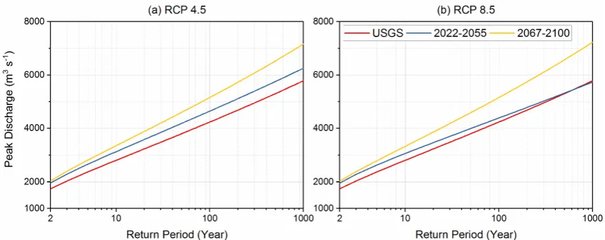
Stevens Pass
(47.7372°N, 121.0914°W)
1241m 1978-1980, 1995-1997, 1999, 2000 8
Tolt S. Fork Reservoir
(47.7000°N, 121.6908°W)
610m 1978-1984, 1986-1988, 1990-1991, 1993,
1995-2000, 2002-2003
21
The RCM includes three groups of climate datasets used to bound the study- historical simulated
125
data (hereafter referred to as historic), and Representative Concentration Pathway 4.5 (RCP4.5) and
126
8.5 (RCP8.5). The historic data is representative of water years 1978 to 2003 and the RCP scenarios
127
represent future time periods (water years: 2022 to 2100). For this study, the future periods were
128
further decomposed into two separate time periods- 2022 to 2055 and 2067 to 2100. The RCM data
129
consisted of hourly data for air temperature, wind speed, relative humidity, incoming shortwave
130
radiation, longwave radiation, and precipitation. These hourly data were aggregated to the 3-hourly
131
format for use by the hydrologic model.
132
2.2. Hydrologic Modeling
133
To translate regional climate data into local-scale runoff distributions, the Distributed
134
Hydrology Soil Vegetation Model (DHSVM) [26] was used to simulate the hydrological processes
135
including precipitation, infiltration, snow accumulation and melt, and runoff at a 3-hourly timescale.
136
The DHSVM model was established for the Snohomish basin at 150-m resolution using the previously
137
DHSVM was further calibrated by adjusting parameters including temperature thresholds
139
impacting rain, snow, and rain-on-snow transitions. In addition, lateral conductivity was used as a
140
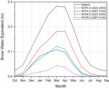
calibration parameter, initially set using published values related to specific soil layers [28] and
141
subsequently uniformly adapted through calibration. Both the temperature thresholds and the lateral
142
conductivity affect the timing and volume of peak runoff.
143
To optimize the hydrologic calibration process, the Multi-objective Complex Evolution Model
144
(MOCOM) [29] was used to fully explore the parameter space and optimize the parameters via an
145
objective function through successive generations of parameters. The objective function for
146
calibration was maximizing fit relative to extreme runoff events, where fit was measured as a function
147
of the coefficient of determination (R2), Nash-Sutcliffe Efficiency (NSE), and the root-mean-square
148
error (RMSE) based on the work of Moriasi et al [30]. The DHSVM calibration and validation period,
149
each a 10-year period, was driven by meteorological observations available in the NLDAS-2 dataset
150
(Figure 3). The calibration and validation point was at a USGS stream gage locations (ID: 12150800
151
Snohomish River near Monroe, WA, U.S.A.) near the downstream end of the basin. The calibrated
152
and validated DHSVM model was rerun using the RCM historic, RCP4.5, and RCP8.5 meteorological
153
forcings under the time periods shown in Table 2.
154
155
156
Figure 3. DHSVM calibration and validation at Monroe, WA.
157
Table 2. Water years used for flow frequency analysis.
158
Scenarios Years
USGS 1964-2015
Historic 1978-2003
RPC4.5 2022-2055, 2067-2100
RPC8.5 2022-2055, 2067-2100
2.3. Frequency Analysis
160
The hydrologic simulations produce a continuous distribution of flows over the duration of the
161
study period. To be able to change relative to flood risk, methods are needed to develop statistical
162
distributions of annual extreme events consistent with engineering design criteria. To this end, the
163
Bulletin 17C method [31] was used to develop statistical extreme event distributions derived from
164
the streamflow simulations generated by DHSVM.
165
There are significant uncertainties in developing future realizations of flood risk with
166
contributions from multiple aspects of the multi-scale, multi-model process [6, 32-37]. For example,
167
while climate models generally do well at representing decadal variability, and to some extent,
168
monthly variability, and representation of annual extremes is challenging.[38-41]. The inability to
169
capture extremes in the meteorological variables translates to an inability to capture extremes in
170
runoff and subsequently an underestimation in statistical distributions of annual extreme events.
171
Because the climate inputs for the Historic and RCP simulations share the same biases and
172
uncertainties, we employ a post frequency analysis bias correction based on differences between the
173
historic simulated data and observed USGS extreme event statistical distributions:
174
= + ( − ), (1)
175
where is the bias-corrected annual extreme flow of an RCP scenario for a given return period
176
event, p; is the annual extreme flow of the derived from USGS instantaneous annual peak
177
flow for a given return period event, p; is the annual extreme flow of an RCP scenario for a
178
given return period event, p, and ℎ is the peak flow of the historic simulated period for a
179
given return period event, p.
180
2.4. Hydrodynamic and Consequence Modeling
181
Statistical distributions representing the change in annual extreme events are not sufficient in
182
developing local-scale, actionable information. To be effective and capture the nonlinearity that exists
183
in flood risk analysis, the statistical distributions of annual extreme flow rates must be translated to
184
spatial estimates of flood extents. To capture the flood extent, a two-dimensional hydrodynamic
185
model based on the shallow water equations is used to characterize extreme event flood behavior.
186
[42]. This model utilizes best-available topographic data and does not require prior knowledge of
187
flow path, effectively able to capture floodplain dynamics.
188
To develop spatial probabilistic risk estimates and capture changes from historic to future
189
climate, samples are taken from across the distributions of extreme events. In this study, nearly 140
190
samples from each statistical distribution (observed and both RCP projections) were taken and each
191
sample was used to drive a hydrodynamic simulation and develop corresponding spatial estimates
192
of flooding. For each hydrodynamic simulation, inundation depths were used to estimate the flood
193
damage and annualized flood risk based on depth-damage fragility curves available from
HAZUS-194
MH [43]. The direct damage can be determined by intersecting the depth from the depth-damage
195
curves to retrieve the percent damage:
196
= ∑ ( , × ), (2)
197
where D is damage ($), g is the spatial aggregation unit (e.g., grid cell for distributed analysis,
198
parcel), n is the total number of the flooded spatial units, h is the flood depth, fcg,h is the percent
199
damage (%) corresponding to the flood depth h from the fragility curve for the gth spatial unit, and
200
SVg is the structural value for the gth spatial unit ($). One U.S. foot (~0.3 m) freeboard was assumed in
201
computing damage since no better information exists to determine the base elevation of a structure
202
[44].
203
Finally, the annualized risk is calculated as the product of damage and the corresponding flood
204
probability [45]:
205
= × , (3)
206
where R is the annualized flood risk, and P is the exceedance probability.
207
As mentioned previously, a definition of spatial aggregation unit and associated monetary value
208
was used to provide the asset value (structural value) for consequence analysis. However, the parcel
210
footprint was not used as the spatial aggregation unit. Rather, an approach was utilized to enhance
211
the spatial resolution of structural representation and avoid estimation of damage in large parcels
212
where the structural footprint is small. To accomplish this, the imperviousness percentages (30 m)
213
from the 2011 U.S. National Land Cover Database was used to filter out the non-developed areas
214
within a parcel. The structural asset value of a given parcel was distributed as a function of
215
imperviousness across the grid cells within the parcel, such that the distributed structural value is
216
conserved when compared to the total parcel value.
217
3. Results and Discussion
218
3.1. Precipitation Analysis
219
Mean-monthly comparisons of precipitation were made to understand the potential cascading
220
bias in the development of local-scale, actionable information. Precipitation from each climate
221
scenario was aggregated to mean-monthly values and compared to the seven weather stations (Table
222
1). The simulated precipitation of the historic scenario appears to over-predict at stations lower than
223
100 m, while generally matched well with the observations at higher elevations (Figure 4). While not
224
fully understood, plausible explanations for this variability is that the areas of the lower elevation are
225
subject to local disturbances (e.g. urban impacts, rain-shadow effect), which were not well captured
226
by the RCM. The precipitation curves from both RCP scenarios are consistently higher when
227
compared to historic precipitation, indicating an increasing trend in the precipitation amount
228
projected for the study area. Notably, both RCP scenarios show increased winter precipitation and
229
decreased summer precipitation relative to the historic scenario, a potentially important shift when
230
considering the potential for changes in rain, snow, and rain-on-snow events and preparation for
231
233
Figure 4. Mean monthly precipitation from seven climate data sets at seven Snohomish watershed locations.
234
3.2. Streamflow Simulation
235
The calibrated and validated DHSVM model was used to predict river flow for both climate
236
scenarios and were subsequently compared to the gauged stream flows representing the current
237
condition. To closely examine the potential impact of the temporal shift in precipitation on the timing
238
of annual peak discharge, five occurrences of maximum daily flow were selected for each year in the
239
future period and compared to the gauge observations. For both the RCP4.5 and the RCP8.5
240
scenarios, there is a clear decrease in the number of months in which peak flows are simulated to
241
occur (Figure 5). That is, there are fewer occurrences of peak flow during the spring and summer
242
months and an increase in the occurrence of peak flows during the winter months. This finding is
243
consistent with the previous observation in this study where projected precipitation extremes tended
244
to shift from spring and summer months to winter months. Comparing the two future scenarios,
245
RCP8.5 scenario tends to have a stronger shift to winter peaks, a potentially important distinction as
246
we compare potential flood risk relative to carbon scenarios.
247
249
Figure 5. The timing of the five largest daily flows in each water year for different scenarios.
250
3.3. Streamflow Frequency Analysis
251
Using the frequency distributions developed using the Bulletin 17C method, direct comparison
252
of annual return period events can be made to quantify relative change in intensity and frequency of
253
extreme flood events. Since traditional frequency analyses such as the Bulletin 17C method implicitly
254
assumed a stationary distribution, each carbon scenario was divided into two time windows. The
255
purpose of this was so as to not dilute future change based on historic conditions. A comparison of
256
the two windows (2022-2055 and 2067-2100), therefore, could directly exhibit the nonstationarity of
257
climate changes (Figure 6). A significant difference between the two future scenarios was found for
258
the period 2022-2055. Compared to RCP4.5, RCP8.5 generally exhibits a smaller increase in peak flows
259
and is especially pronounced for the more extreme return period events, consistent with previous
260
findings [46]. Although the projected peak flows of our RCP8.5 scenario became even slightly lower
261
than the historic conditions for the largest return periods, this was also found by a previous study
262
using 10 GCMs since simulating rare events with the large return periods is always challenging [46]
263
(page 181). Because the occurrence of precipitation peaks and runoff peaks are projected to toward
264
winter months, this finding could be expected to be related to the timing of rain-on-snow events. The
265
potential implications of rain-on-snow events will be discussed in details later.
266
The later future period (2067-2100) for both scenarios all show an increase in peak river flow
267
when compared to the early future period (2022-2055) (Figure 6). This exposes a nonstationary
268
condition in the magnitude of peak discharges for a given flood probability, and conversely, a
269
nonstationary reduction in the return interval for given peak discharge. These nonstationary changes
270
could be expected to be more intense for the rarer but more severe floods and, therefore, be associated
271
with more significant consequences.
272
An example can be given to take a closer look at these nonstationary changes. The low end of
273
events (and therefore more certainty) than the high end of the return periods established based on
275
few, rare events (Figure 6). Among the selected six return periods shown in Figure 7, both climate
276
scenarios projected a larger magnitude of peak flows for a same historic return period. That is, the
277
new 10-year return period in RCP4.5 and RCP8.5 could have more than 9% increase in the peak flows
278
when compared historically. Conversely, the historic 10-year peak flow would be expected to
279
happen, on average, every 5-7 years under both climate scenarios. Even within the selected 200-year
280
time window, the nonstationarity was clearly exhibited with a reverse changing trend between the
281
two periods; i.e. the percent increases in the peak discharges for both RCP4.5 and RCP8.5 scenarios
282
were projected to keep shrinking during 2022-2055 along with the return period, while the percent
283
increase in peak discharges for both scenarios kept enlarging during 2067-2100.
284
285
Figure 6. Frequency curves of annual peak flow at Monroe for USGS instantaneous observations (1964-2014),
286
RCP4.5 (a), and RCP8.5 (b) made by the Bulletin 17C method.
287
288
Figure 7. Percent increase of estimated future peak flows for RCP4.5 (a) and RCP8.5 (b) over the historic USGS
289
instantaneous peak flows.
290
3.4. Peak flows and the role of rain-on-snow events
291
Given the general perception of increased impacts for more extreme climate scenarios, it may be
292
somewhat non-intuitive to expect the reduced potential for flooding under warmer climate
293
conditions. Peak flows in a river have a complex, nonlinear relationship with precipitation dynamics.
294
Peak flows can be driven by rain events, snowmelt freshets, or rain-on-snow events. To understand
295
the influence of climate scenario of peak flow, snow water equivalent (SWE) (Figure 8) and the
296
events, changes were quantified by calculating the amount of dime that rain-on-snow events
298
occurred at 5 locations and normalizing each location to the historic period.
299
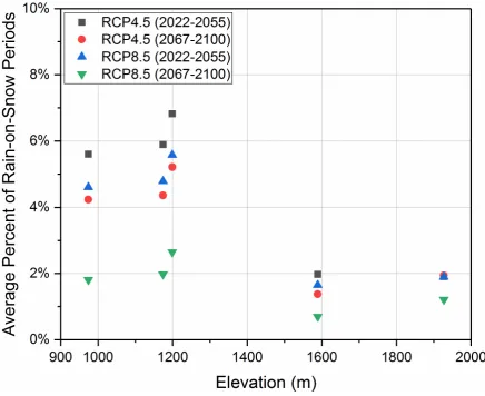
300
302
Figure 9. The percent of occurrence of rain-on-snow events occurred at 5 randomly selected elevations.
303
Relative to the historic scenario, all RCP pathways had a decreased snow water equivalent
304
(SWE), which means a larger fraction of the precipitation fell as rain. Considering that the
305
precipitation peaks were projected to shift more towards winter months, more rain and rain-on-snow
306
events were projected to happen considering an increase in temperature. This would tend to reduce
307
snowmelt-driven peak flows in the springtime but trigger more intensive rain and rain-on-snow
308
driven peak flow events. However, both time periods of the RCP8.5 scenario exhibited less SWE than
309
RCP4.5 (Figure 8), indicating a more intensive reduction in the snowpack and reducing the potential
310
for rain-on-snow occasions in the RCP8.5. Particularly, the second period (2067-2100) of RCP8.5 had
311
the least amount of snowpack (Figure 8) and the least occurrence of rain-on-snow events (Figure 9)
312
due to increase in temperature in which case the snowpack may melt before being compounded with
313
the upcoming winter storms. This could explain why the second period of RCP8.5 had larger peak
314
flows (Figure 6), which would be only in response to rainfall as found by Madsen et al [47].
315
Surprisingly, the first period (2022-2055) of RCP8.5 had the moderate amount of remaining SWE
316
(Figure 8) and frequent rain-on-snow events (Figure 9) but the reduced peak-flow magnitudes (Figure
317
6), which was also found by multiple previous studies as summarized by Madsen et al [47]. The
318
reason for these similar declined flood magnitudes is still not clear, but they should be related to the
319
timing and the conversion between rain and snow.
320
3.5. Quantification of Consequences
321
The end products of the integrated multi-scale, multi-model framework quantify the flood risk
322
at a local scale. In this case, only the later time period is considered when evaluating future flood risk.
323
The frequency distribution for the two climate scenarios for the later time period is shown in Figure
324
RCP4.5. Therefore, RCP4.5 represents the more severe flow condition in this study case, while RCP8.5
326
would fall within the envelope bounded by USGS and RCP4.5.
327
To capture the most extreme chance for change under future climate scenarios, only the USGS
328
(used as a baseline) and RCP4.5 frequency distributions were used. Due to the projected climate
329
change (from USGS to RCP4.5), the studied watershed would experience 24%, 33%, 29% increases in
330
both damage and annualized risk (with the same rates) for the 10-year, 100-year, and 1000-year floods
331
(Figure 11). The maximum annualized flood risk was raised by 15% from the USGS condition to
332
RCP4.5 condition, while both of the maximums occurred at the 1.2-year flood, indicating that the
333
mitigation measures should most target the repetitive low-risk floods for this region. The damage
334
caused by the historic 10-year flood would be expected to be equivalent to damage of the new 5-year
335
flood in the projected future climate, while the damage caused by the historic 100-year flood would
336
be projected to the only amount to the damage of the new 29-year flood. This indicates the necessity
337
to incorporate the climate change into the strategic planning to manage the future flood management.
338
339
Figure 10. Frequency curves of annual peak flow with combined two periods for USGS instantaneous
340
observations, RCP4.5 (a), and RCP8.5 (b) made by the Bulletin 17C method.
341
342
4. Conclusions
344
The primary outcome of this project is the demonstration of the ability to utilize regional-scale
345
climate data to develop local-scale runoff distributions that can be used for community and
346
infrastructure planning. While the focus of this project was extreme precipitation and runoff relative
347
to flooding, the same approach can be utilized to investigate water management strategies relative to
348
temporal shifts in annual runoff volume under water-stressed conditions.
349
Major findings of this study can be summarized as follows.
350
(1) The peak flows simulated by the proposed model chain have been calibrated and validated
351
by compared to the observation;
352
(2) The peaks of precipitation and streamflows were projected to shift from spring and summer
353
to the earlier winter season;
354
(3) The nonstationarity of peak discharges was exhibited from both RCP4.5 and RCP8.5
355
scenarios with more frequent and severe flood risks projected in the longer future.
356
(4) The RCP 4.5 pathway projected overall higher peak flows than the RCP 8.5 pathway for the
357
study region, where more rain-on-snow events projected by RCP4.5 might be the reason.
358
359
Acknowledgments: This work was mainly sponsored by Pacific Northwest National Laboratory (PNNL)
360
Laboratory Directed Research and Development program. PNNL is operated for U.S. Department of Energy by
361
Battelle Memorial Institute under contract DE-AC05-76RL01830. The work also received kind supports from the
362
Snohomish County, WA, U.S.
363
Author Contributions: D.J. conceived and designed the project; D.J. and C.R. performed the model; S.W., D.J.,
364
Y.F., and C.R. analyzed the data; D.J., Y.F., and C.R. wrote the paper. Authorship must be limited to those who
365
have contributed substantially to the work reported.
366
Conflicts of Interest: The authors declare no conflict of interest.
367
References
368
1. Fowler, H.J.; Wilby, R.L. Detecting changes in seasonal precipitation extremes using regional climate
369
model projections: Implications for managing fluvial flood risk.Water Resources Research, 2010. 46(3).
370
2. Cheng, L.; AghaKouchak, A. Nonstationary precipitation intensity-duration-frequency curves for
371
infrastructure design in a changing climate.Scientific reports, 2014. 4: p. 7093.
372
3. Mailhot, A.; Duchesne, S. Design Criteria of Urban Drainage Infrastructures under Climate Change.
373
Journal of Water Resources Planning and Management, 2010. 136(2): p. 201-208.
374
4. Kim, B.S.; Kim, B.K.; Kwon, H.H. Assessment of the impact of climate change on the flow regime of the
375
Han River basin using indicators of hydrologic alteration.Hydrological Processes, 2011. 25(5): p. 691-704.
376
5. Wood, A.W.; Leung, L.R.; Sridhar, V.; Lettenmaier, D.P. Hydrologic Implications of Dynamical and
377
Statistical Approaches to Downscaling Climate Model Outputs.Climatic Change, 2004. 62(1): p. 189-216.
378
6. Prudhomme, C.; Jakob, D.; Svensson, C. Uncertainty and climate change impact on the flood regime of
379
small UK catchments.Journal of Hydrology, 2003. 277(1-2): p. 1-23.
380
7. Dulie, V.; Zhang, Y.; Salathe, E.P. Extreme precipitation and temperature over the U.S. Pacific Northwest:
381
A comparison between observations, reanalysis data, and regional models.Journal of Climate, 2011. 24(7):
382
p. 1950-1964.
383
8. Fowler, H.J.; Blenkinsop, S.; Tebaldi, C. Linking climate change modelling to impacts studies: recent
384
advances in downscaling techniques for hydrological modelling.International Journal of Climatology, 2007.
385
27(12): p. 1547-1578.
386
9. Xu, C.-y. From GCMs to river flow: a review of downscaling methods and hydrologic modelling
387
10. Prudhomme, C.; Reynard, N.; Crooks, S. Downscaling of global climate models for flood frequency
389
analysis: where are we now? Hydrological Processes, 2002. 16(6): p. 1137-1150.
390
11. Sunyer, M.A.; Hundecha, Y.; Lawrence, D.; Madsen, H.; Willems, P.; Martinkova, M.; Vormoor, K.; Bürger,
391
G.; Hanel, M.; Kriaučiuniene, J.; Loukas, A.; Osuch, M.; Yücel, I. Inter-comparison of statistical
392
downscaling methods for projection of extreme precipitation in Europe. Hydrology and Earth System
393
Sciences, 2015. 19(4): p. 1827-1847.
394
12. Burton, A.; Fowler, H.J.; Blenkinsop, S.; Kilsby, C.G. Downscaling transient climate change using a
395
Neyman-Scott Rectangular Pulses stochastic rainfall model.Journal of Hydrology, 2010. 381(1-2): p. 18-32.
396
13. Vormoor, K.; Lawrence, D.; Heistermann, M.; Bronstert, A. Climate change impacts on the seasonality and
397
generation processes of floods - Projections and uncertainties for catchments with mixed
398
snowmelt/rainfall regimes.Hydrology and Earth System Sciences, 2015. 19(2): p. 913-931.
399
14. Mizukami, N.; Clark, M.P.; Gutmann, E.D.; Mendoza, P.A.; Newman, A.J.; Nijssen, B.; Livneh, B.; Hay,
400
L.E.; Arnold, J.R.; Brekke, L.D. Implications of the Methodological Choices for Hydrologic Portrayals of
401
Climate Change over the Contiguous United States: Statistically Downscaled Forcing Data and
402
Hydrologic Models.Journal of Hydrometeorology, 2016. 17(1): p. 73-98.
403
15. Camici, S.; Brocca, L.; Moramarco, T. Accuracy versus variability of climate projections for flood
404
assessment in central Italy.Climatic Change, 2017: p. 1-14.
405
16. Khaliq, M.N.; Ouarda, T.B.M.J.; Ondo, J.C.; Gachon, P.; Bobée, B. Frequency analysis of a sequence of
406
dependent and/or non-stationary hydro-meteorological observations: A review.Journal of Hydrology, 2006.
407
329(3): p. 534-552.
408
17. Teng, J.; Jakeman, A.J.; Vaze, J.; Croke, B.F.W.; Dutta, D.; Kim, S. Flood inundation modelling: A review
409
of methods, recent advances and uncertainty analysis.Environmental Modelling & Software, 2017. 90: p.
201-410
216.
411
18. Kalyanapu, A.; Judi, D.; McPherson, T.; Burian, S. Monte Carlo-based flood modelling framework for
412
estimating probability weighted flood risk.Journal of Flood Risk Management, 2012. 5(1): p. 37-48.
413
19. Snohomish County. Hazard Mitigation Plan: Summary. 2015.
414
20. Hamlet, A.F. Assessing water resources adaptive capacity to climate change impacts in the Pacific
415
Northwest Region of North America.Hydrology and Earth System Sciences, 2011. 15(5): p. 1427-1443.
416
21. Kraucunas, I.; Clarke, L.; Dirks, J.; Hathaway, J.; Hejazi, M.; Hibbard, K.; Huang, M.; Jin, C.;
Kintner-417
Meyer, M.; van Dam, K.K. Investigating the nexus of climate, energy, water, and land at decision-relevant
418
scales: the Platform for Regional Integrated Modeling and Analysis (PRIMA).Climatic Change, 2015. 129
(3-419
4): p. 573-588.
420
22. Gao, Y.; Leung, L.R.; Lu, J.; Liu, Y.; Huang, M.; Qian, Y. Robust spring drying in the southwestern US and
421
seasonal migration of wet/dry patterns in a warmer climate.Geophysical Research Letters, 2014. 41(5): p.
422
1745-1751.
423
23. Skamarock, W.C.; Klemp, J.B.; Dudhia, J.; Gill, D.O.; Barker, D.M.; Duda, M.G.; Huang, X.-y.; Wang, W.;
424
Powers, J.G. A description of the advanced research WRF version 3, in NCAR Tech. Note. 2008, Natl. Cent.
425
for Atmos. Res.: Boulder, Colo., U.S.A.
426
24. Xia, Y.; Mitchell, K.; Ek, M.; Sheffield, J.; Cosgrove, B.; Wood, E.; Luo, L.; Alonge, C.; Wei, H.; Meng, J.;
427
Livneh, B.; Lettenmaier, D.; Koren, V.; Duan, Q.; Mo, K.; Fan, Y.; Mocko, D. Continental-scale water and
428
energy flux analysis and validation for the North American Land Data Assimilation System project phase
429
2 (NLDAS-2): 1. Intercomparison and application of model products. Journal of Geophysical Research:
430
25. Hejazi, M.I.; Voisin, N.; Liu, L.; Bramer, L.M.; Fortin, D.C.; Hathaway, J.E.; Huang, M.; Kyle, P.; Leung,
432
L.R.; Li, H.-Y. 21st century United States emissions mitigation could increase water stress more than the
433
climate change it is mitigating.Proceedings of the National Academy of Sciences, 2015. 112(34): p. 10635-10640.
434
26. Wigmosta, M.S.; Vail, L.W.; Lettenmaier, D.P. A distributed hydrology-vegetation model for complex
435
terrain.Water resources research, 1994. 30(6): p. 1665-1679.
436
27. Yang, Z.; Wang, T.; Voisin, N.; Copping, A. Estuarine response to river flow and sea-level rise under future
437
climate change and human development.Estuarine, Coastal and Shelf Science, 2015. 156: p. 19-30.
438
28. Maidment, D.R. Handbook of hydrology. Vol. 1. 1993: McGraw-Hill New York.
439
29. Yapo, P.O.; Gupta, H.V.; Sorooshian, S. Multi-objective global optimization for hydrologic models.Journal
440
of hydrology, 1998. 204(1-4): p. 83-97.
441
30. Moriasi, D.N.; Arnold, J.G.; Van Liew, M.W.; Bingner, R.L.; Harmel, R.D.; Veith, T.L. Model evaluation
442
guidelines for systematic quantification of accuracy in watershed simulations.Transactions of the ASABE,
443
2007. 50(3): p. 885-900.
444
31. England Jr, J.F.; Cohn, T.A.; Faber, B.A.; Stedinger, J.R.; Thomas Jr, W.O.; Veilleux, A.G.; Kiang, J.E.; Mason
445
Jr, R.R. Guidelines for determining flood flow frequency—Bulletin 17C. 2018, US Geological Survey.
446
32. Brigode, P.; Bernardara, P.; Paquet, E.; Gailhard, J.; Garavaglia, F.; Merz, R.; Mic̈ovic̈, Z.; Lawrence, D.;
447
Ribstein, P. Sensitivity analysis of SCHADEX extreme flood estimations to observed hydrometeorological
448
variability.Water Resources Research, 2014. 50(1): p. 353-370.
449
33. Qi, W.; Zhang, C.; Fu, G.; Zhou, H.; Liu, J. Quantifying Uncertainties in Extreme Flood Predictions under
450
Climate Change for a Medium-Sized Basin in Northeastern China.Journal of Hydrometeorology, 2016. 17(12):
451
p. 3099-3112.
452
34. Hundecha, Y.; Sunyer, M.A.; Lawrence, D.; Madsen, H.; Willems, P.; Bürger, G.; Kriaučiūnienė, J.; Loukas,
453
A.; Martinkova, M.; Osuch, M.; Vasiliades, L.; von Christierson, B.; Vormoor, K.; Yücel, I. Inter-comparison
454
of statistical downscaling methods for projection of extreme flow indices across Europe. Journal of
455
Hydrology, 2016. 541, Part B: p. 1273-1286.
456
35. Jiang, P.; Gautam, M.R.; Zhu, J.; Yu, Z. How well do the GCMs/RCMs capture the multi-scale temporal
457
variability of precipitation in the Southwestern United States? Journal of Hydrology, 2013. 479: p. 75-85.
458
36. Camici, S.; Brocca, L.; Melone, F.; Moramarco, T. Impact of climate change on flood frequency using
459
different climate models and downscaling approaches.Journal of Hydrologic Engineering, 2014. 19(8).
460
37. Condon, L.E.; Gangopadhyay, S.; Pruitt, T. Climate change and non-stationary flood risk for the upper
461
Truckee River basin.Hydrology and Earth System Sciences, 2015. 19(1): p. 159-175.
462
38. Seidou, O.; Ramsay, A.; Nistor, I. Climate change impacts on extreme floods I: Combining imperfect
463
deterministic simulations and non-stationary frequency analysis.Natural Hazards, 2012. 61(2): p. 647-659.
464
39. Kourgialas, N.N.; Dokou, Z.; Karatzas, G.P. Statistical analysis and ANN modeling for predicting
465
hydrological extremes under climate change scenarios: The example of a small Mediterranean
agro-466
watershed.Journal of Environmental Management, 2015. 154: p. 86-101.
467
40. Jaw, T.; Li, J.; Hsu, K.L.; Sorooshian, S.; Driouech, F. Evaluation for Moroccan dynamically downscaled
468
precipitation from GCM CHAM5 and its regional hydrologic response. Journal of Hydrology: Regional
469
Studies, 2015. 3: p. 359-378.
470
41. Lu, Y.; Qin, X.S.; Xie, Y.J. An integrated statistical and data-driven framework for supporting flood risk
471
analysis under climate change.Journal of Hydrology, 2016. 533: p. 28-39.
472
42. Judi, D.R.; Burian, S.J.; McPherson, T.N. Two-dimensional fast-response flood modeling: Desktop parallel
473
43. Scawthorn, C.; Flores, P.; Blais, N.; Seligson, H.; Tate, E.; Chang, S.; Mifflin, E.; Thomas, W.; Murphy, J.;
475
Jones, C.; Lawrence, M. HAZUS-MH Flood Loss Estimation Methodology. II. Damage and Loss
476
Assessment.Natural Hazards Review, 2006. 7(2): p. 72-81.
477
44. FEMA. Technical Bulletin 10: Ensuring that structures built on fill in or near special flood hazard areas are
478
reasonably safe from flooding. 2001.
479
45. Kalyanapu, A.J.; Judi, D.R.; McPherson, T.N.; Burian, S.J. Annualised risk analysis approach to
480
recommend appropriate level of flood control: application to Swannanoa river watershed.Journal of Flood
481
Risk Management, 2015. 8(4): p. 368-385.
482
46. Snohomish County. Hazard Mitigation Plan: Volume 1 Risk Assessment. 2015.
483
47. Madsen, H.; Lawrence, D.; Lang, M.; Martinkova, M.; Kjeldsen, T.R. Review of trend analysis and climate
484
change projections of extreme precipitation and floods in Europe.Journal of Hydrology, 2014. 519: p.
3634-485