CENTRE FOR
COMPUTING AND BIOMETRICS
Convexity-preserving B-spline
modification
Tim N.T. Goodman and Keith Unsworth
Research Report No:97/07
October 1997
L I N C O L N
U N I V E R S I T Y
R
ESEARCH
E
R
PORT
Centre for Computing and Biometrics
The Centre for Computing and Biometrics (CCB) has both an academic (teaching and research) role and a computer services role. The academic section teaches subjects leading to a Bachelor of Applied Computing degree and a computing major in the BCM degree. In addition it contributes computing, statistics and mathematics subjects to a wide range of other Lincoln University degrees. The CCB is also strongly involved in postgraduate teaching leading to honours, masters and PhD degrees. The department has active research interests in modelling and simulation, applied statistics and statistical consulting, end user computing, computer assisted learning, networking, geometric modelling, visualisation, databases and information sharing.
The Computer Services section provides and supports the computer facilities used throughout Lincoln University for teaching, research and administration. It is also responsible for the telecommunications services of the University.
Research Report Editors
Every paper appearing in this series has undergone editorial review within the Centre for Computing and Biometrics. Current members of the editorial panel are
Dr Alan McKinnon Dr Bill Rosenberg Dr Clare Churcher Dr Jim Young
Dr Keith Unsworth Dr Don Kulasiri Mr Kenneth Choo
The views expressed in this paper are not necessarily the same as those held by members of the editorial panel. The accuracy of the information presented in this paper is the sole responsibility of the authors.
Copyright
Copyright remains with the authors. Unless otherwise stated, permission to copy for research or teaching purposes is granted on the condition that the authors and the series are given due acknowledgement. Reproduction in any form for purposes other than research or teaching is forbidden unless prior written permission has been obtained from the authors.
Correspondence
This paper represents work to date and may not necessarily form the basis for the authors' fmal conclusions relating to this topic. It is likely, however, that the paper will appear in some form in a journal or in conference proceedings in the near future. The authors would be pleased to receive correspondence in connection with any of the issues raised in this paper. Please contact the authors either by email or by writing to the address below.
Any correspondence concerning the series should be sent to: The Editor
Centre for Computing and Biometrics PO Box 84
Lincoln University
Convexity-preserving B-spline modification
Tim N.T. Goodman* and Keith Unsworth#
*Department of Mathematics and Computer Science, University of Dundee, Dundee DD1 4HN, SCOTLAND.
email: [email protected]
#Centre for Computing and Biometrics, Lincoln University,
Canterbury, NEW ZEALAND. email: [email protected]
Abstract
We consider the problem of modifying the shape of a cubic B-spline curve while retaining its convexity. This is achieved by moving control points in such a way as to maintain the appropriate shape of the corresponding control polygon. The problem is formulated as a linear programming problem, which may be solved using the simplex method. Two examples, taken from cross-sections of a ship hull, are discuss~d.
1
Introduction
It is well known that C2 continuous parametric curves may be constructed using cubic
splines, using B-splines as the corresponding basis [Farin 97]. The provision of cubic B-splines as a standard component of Computer Aided Design software is now common-place, with implementations widely available using both the polynomial form and the rational form (NURBS) [Piegl & Tiller 97].
In this paper, we consider the problem of generating and subsequently modifying a poly-nomial cubic B-spline curve in which the control polygon is locally convex and is of an appropriate shape in order that the curve itself is convex. Hence the problem of mod-ifying this curve is one in which control points can only be moved in such a way as to maintain this shape. In the following sections we formulate this as a linear programming problem, which may be solved using the simplex method.
The outline of the paper is as follows. In §2 necessary and sufficient conditions are derived in order for a Bezier curve segment to be convex. These conditions are then related to the corresponding B-spline control points. The linear programming problem is formulated in §3 and the steps of a "simple" algorithm to solve this problem are presented in §4. An additional algorithmic step is suggested in §5, which offers a further chance of obtaining a solution in the event that a solution is not obtained using the "simple" algorithm. Two sets of results are described in §6, with each set taken from the design of cross-sections of a ship hull. The paper concludes with §7.
2
Convexity Conditions
In this section we derive necessary and sufficient conditions for a cubic Bezier curve to be convex, i.e. for the curvature to be everywhere non-negative. These conditions are then written in terms of the corresponding B-spline control points.
Consider a cubic curve in ~2 written in Bezier form:
r(t) = A(l - t)3
+
3B(1 - t)2t+
3C(1 - t)t2+
Dt3, 0:::; t :::; 1. (1)Writing
we have
r' (
t)
X r"(t )
18
where
E
=
B - A, F=
C - B, G=
D - C,(E(I- t)2
+
2Ft(1- t)+
Gt2) x ((F - E)(I-t)+ (G -
F)t)(1 - t)3(E x F)
+
t(1 - t)2(E x (F+
G))+
t2(1-
t)((E+
F) x G)+
t3(F x G)(2)
(1 - t)2(E x F)
+
t(1 - t)(E x G)+
t2(F x G), 0 :::; t :::; 1, (3)Now take k
2:
4, and an increasing sequence of knots u = (Ui)~tl. For the purposes of this paper we will assume this sequence to be strictly increasing. For i = 0, ... ,k - 1 we let Ni denote the cubic B-spline with knots Ui-2, . . . ,Ui+2·Consider a cubic B-spline curve
k-l
r(u)
=
L
BiNi(u),
(4)On the interval [Uj, Uj+l],
1:S
j:S
k -3, (4)
may be written in Bezier form(1)
where: and A B C D tFrom (2), (5) we obtain
where
Hence from (3), (6),
r' (
t) x r" ( t )
18 6 j I5j rPj Cij j3j '"'(j E F G L M N J-L
Uj+l - Uj,
Uj+l - Uj-l,
Uj+2 - Uj-l,
6~ J
I5j rPj-l
,
6 jl5j - 1 6j - II5HI
+
I5j rPj-1 I5j rPj
6~ I
~
I5j rPj
- L+M,
}
- J-LM,
- M+N,
Cij(B j - B j - I ),
~i~i-l fj-¢>- (B HI - B ) j ,
J J
'"'(j(B H2 - BHI ),
~
~j-l .
(1 - t)2(L x M) + ;t(1 - t)(L x M + Lx N + M x N) + t2(M x N),
(5)
(6)
o
:S
t:S
1.(7)
Noting that J-L
>
0, it follows from (7) thatr' (t) x r" (t)
2::
0,if and only if
Lx M
>
0,M x N
>
0,O:St:Sl,
L x M + L x N + M x N
> -
2J-LV (L x M) (M x N).(8)
Thus while the control polygon Bj - I , . .. ,BH2 is locally convex, in the event that it turns
3
The Linear Programming Problem
We now consider the problem of moving control points in order to change the shape of the curve while retaining its convexity properties. This is formulated as the linear programming problem (11).
Take s,
0:::;
s :::;1
and suppose that the curve r(t) is initially given by(1), (5).
We wish to move r(s) a given distance D in the direction of a given vector v = (vx, vy). We do this by allowing at most four control points to be adjusted. Thus, we replaceBi by Bi+AiV, i=j-1, ... ,j+2.
Then from (1) and (5) we obtain
D = Ivl{Aj-IO!j(l-s?
+
Aj((3j(l -3)3
+3D~+l
s(l - s? + 3,0.j+l s2(1 - s) + O!j+lS3)~j CPj
( (
)3
,0.j-1 ()2
Dj 2 ( )
3)
+
Aj+1 Ij 1 - 3 + 3 - " , - 3 1 - 3 + 3-s 1 - s + (3j+IS~j CPj
+
Aj+2Ij+l33}. (9)We assume that initially the curve is locally convex over the region influenced by the control points Bj - I , ... ,Bj+2' i.e.
r'(u) x r"(u)
2:
0, -Uj-3 :::; U :::; Uj+4' In particular the discrete curvaturesKi = (Bi - B i- I) X (BHI - B i), i = j - 3, ... ,j
+
4,satisfy
(10)
If the original inequalities have the opposite sign we reverse the order of the Bi and the corresponding knots. Noting that the knots should form an increasing sequence, the
signs of the knots should also be changed.
Letting Bi - B i- I = (Xi, Yi), (10) becomes
i = j - 3, ... ,j
+
4. For i = j - 2, ... ,j+
3, let the new discrete curvatures be given byK;
(Bi + AiV - B i- I - Ai-IV) X (BHI + AHIV - Bi - AiV)= XiYi+l - XHIYi
+
(Ai - Ai-I)(VxYi+l - VyXHI )+ (AHI - Ai) (VyXi - vxYi).
We require the new curve to be locally convex on [Uj-3, Uj+41. It is generated by moving the control points such that no individual discrete curvature increases significantly in excess of the others. To achieve this, we
maximise {. . min.
K; }
~=J-2, ... ,J+3
by varying Aj-I, ... , Aj+2 subject to (9). This is equivalent to the following linear pro-gramming problem:
4
The Algorithm
In this section a simple algorithm is proposed in order to solve (8) and (11).
1. Let .\ = 0 for i ::; j - 1 and i
2:
j + 2.2. Calculate Aj, Aj+! in order to solve (11).
3. For i = j, j + 1, let
(Note that
K/'
= Li x Li+d4. If K
<
0 then go to step 5 else (a) iffori=j-2, ... ,j+2(12)
then STOP, else
(b) if for i = j - 2, ... j + 2
(Li X Li+l
+
Li X Li+2+
Li+l X Li+2)2::; 4/1?(Li X Li+l)(Li+l x Li+2), (13)
then STOP, else go to step 5.
5. Let Ai = 0 for i ::; j - 2 and i
2:
j + 3.7. If K
<
0 then STOP, else(a) if, for i = j - 3, ... j + 3, (12) is satisfied then STOP, else
(b) if, for i = j - 3, ... j + 3, (13) is satisfied then STOP.
5 An Extended Algorithm
In the event that the above algorithm produces a solution which satisfies (11), but which fails to satisfy either (12) or (13), a further step could be added based upon the following sufficient conditions for (8):
N x L
:s;
2(p,
+
l)(L x M), } (14)N
x
L:s;
2(p,
+
l)(Mx
N).These conditions are clearly sufficient if L x N
2:
O. Otherwise,VN xL:S;
(j2(p,+
l)(L x M),j2(p,
+
l)(M x N)). and so
N x L
<
2(p,+
l)j(L x M)(M x N)<
L x M+
M x N+
2P,V'-(L-x-M-)-(M-x-N-)and (8) follows.
We may therefore add the following step to the algorithm, following step 7 above.
Step 8. Calculate Aj-l, Aj, Aj+l, Aj+2 to
maximise {P} subject to
equation (9), }
Kt2:0, i=j-2, ... ,j+3,
P
:s;
L'i X Li+2+
2(p,
+
l)(Lkx
Lk+l), i = j - 3, ... ,j+
3;k
=
i, i+
l.We note that if P
2:
0, then by (14), the curve is locally convex on [Uj-3, uj+4l.6
Results
We present the results obtained from applying the above algorithm to two test cases. Each set of data represents a cross-section of a ship hull.
Case 1
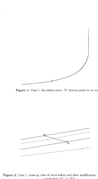
This comprises a non-uniform B-spline using 22 control points. The original curve is shown in figure 1, with 'X' denoting the location of the point to be moved. The corre-sponding polygon is also displayed as a dashed line, but much of it is coincident with the curve. The point 'X' almost coincides with the location of a knot, Its coordinates are (2.5, 4.1590), and it needs to be moved to (2.52,4.1520), Thus in the notation of §3,
v
=
(vx, vy) = (0.02, -0.007) and D = 0.0211896.Figure 1: Case 1: the initial curve. 'X' denotes point to be moved.
---
--- -
....
----
-
---
/
...
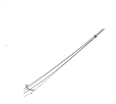
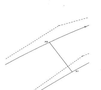
Figure 3: Case 1: sections of curves before and after modification. The two control points which move are shown.
Case 2
This comprises a non-uniform B-spline using 106 control points. The original curve is shown in figure 4, with 'X' denoting the location of the point to be moved. The corresponding polygon is also displayed, but is virtually coincident with the curve. The actual coordinates of the point 'X' are (-0.6998, 2.15221). The original requirement was to move this point to (-0.7698, 2.32). Thus in the notation of §3, v
=
(vx,Vy)
= (-0.07,0.16479) and D = 0.17904. Application of the algorithm failed to find a solution to this problem if only four control points (at most) are allowed to move. By allowing just four control points to move in the given direction, 98% of the distance was covered, with D = 0.1745.Figure 4: Case 2: the initial curve. 'X' denotes point to be moved.
,-,-'- X1
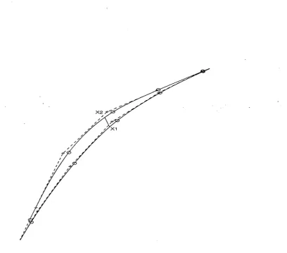
Figure 5: Case 2: close-up view of curve before and after modification. Point on curve
Figure 6: Case 2: sections of curves before and after modification. The four control points which move are shown.
7
Conci usions
We have presented a simple algorithm for modifying the shape of a cubic B-spline curve while retaining its convexity. There are further tests which may be performed to assess the properties of the existing algorithm, and further aspects which may be explored to develop a more versatile algorithm. These include the following.
1. It is well known that linear programming problems do not always yield unique solutions. In such cases a designer would therefore have a selection of possible curves from which to choose. While this offers some flexibility, it may also serve to confuse. Experimentation with a different (non-linear) formulation has yet to be performed.
2. The question of accumulated modifications has yet to be investigated, e.g. are two consecutive modifications equivalent to one modification of the combined distance?
in different directions would increase both the flexibility and complexity of the algorithm,
Each of these remain a subject of further study,
Acknowledgments
We are grateful to Kockums Computer Systems UK for supplying the data for the two test cases described in this paper, In particular we wish to acknowledge the work of Andy Ives-Smith and Ian Applegarth for suggesting the problem and for providing prompt assistance as and when required,
Tim Goodman also acknowledges financial support provided by the European Union via the FAIRSHAPE Human Capital and Mobility project,
References
[Farin 97] Farin, G" (1997) Curves and Surfaces for Computer Aided Geometric De-sign,4th ed" Academic Press, San Diego,
[Piegl & Tiller 97] Piegl, L, and Tiller, W" (1997) The NURBS book, 2nd ed" Springer-Verlag, Berlin,